1. Introduction
Advanced wireless broadband technology has introduced an unprecedented data traffic upgrade in the vehicular networks (VNET). This aims to improve safety and fuel economy and reduce traffic congestion in the transportation system. To cope with these challenges, the offloading of tasks to road side units (RSU) has been proposed to improve quality-of-service (QoS), although a large number of computation is carried out during difficult deadline [
1,
2]. Nowadays, mobile smart devices become a common tool for social networks such as entertainment, learning, and smart life [
3,
4]. While mobile applications continue to emerge and computing power is becoming more and more dense, due to resource constraints of mobile devices (e.g., battery life and storage capacity), the computing power of mobile devices is still limited. This makes mobile users unable to achieve the same satisfaction as desktop users [
5]. A more effective way to improve the performance of mobile device programs is to offload some of their tasks to the remote cloud [
6,
7]. However, the cloud is usually far from the mobile device, resulting in long data transmission delays between mobile devices and unpredictable results [
8,
9]. This is not good for mobile device programs that respond immediately. Time is of the utmost importance to mobile users, such as augmented reality apps and mobile multi-player gaming systems. To overcome the challenges mentioned above, mobile edge computing [
10,
11] (MEC) enables mobile devices to access their internal applications and serve a variety of wireless access networks [
12,
13]. This approach also enables computing tasks from the core network to be transmitted to the edge network to reduce latency. In view of some characteristics of MEC technology, multiple types of access technologies have been allowed, so vehicles can access MEC servers through various base stations (BS), such as Wi-Fi access points (Wi-Fi APs), RSU, and evolved NodeBs (eNBs).
In this paper, we assume that each edge server has the same limited resources to handle the request of the mobile vehicle, i.e., each edge server has the same processing power and these servers are arranged at certain BS locations for mobile vehicle access. We treat multiple vehicles as multiple computing tasks. Multi computing tasks scheduling problem is analogous to multi task learning (MTL) model. Due to the sharing process that produces data, even real-world tasks that appear to be unrelated have strong dependencies. This causes the application of multiple tasks to become the inductive bias in the learning model. Therefore, a multi-task scheduling (MTS) system is a model with a set of input points (co-located positions) and a set of tasks (mobile vehicles) with a variety of targets. The general workaround to construct a cross-task inductive bias is to generate a set of hypotheses that share some parameterization between tasks. In a typical MTS system, we learn its parameters by solving an optimization problem that attempts to minimize the weighted sum of the empirical losses for each task. Notice that the linear combination form makes sense if and only if the parameter set is valid in all tasks. Namely, the weighted sum of empirical loss minimization is effective only if the tasks are non-competing. However, this rarely happens. In other words, MTS is to trade-off competing objectives and merely by linear combinations will not reach the goal.
Another objective of MTS is to find solutions that are not subject to any other. This solution is denoted as the Pareto optimal. In our work, we present Pareto optimal solution for the MTS target. Finding the Pareto optimal solution that subject to a variety of quantization restraint is referred to as multi-objective optimization (MOO). There are several algorithms to solve MOO. One of these methods is called the Multi Gradient Descent Algorithm (MGDA). MGDA optimizes on the basis of gradient descent, and verifies the points that converge to the Pareto set [
14]. MGDA is ideal for multi-task in deep networks. It takes advantage of the gradient of each task and solves the optimization problem while determining updates over global parameters. However, the large-scale application of MGDA is still impractical due to two technical issues. (1) Potential optimization problems cannot be extended to high dimensional gradients better, but this naturally occurs in deep networks. (2) The algorithm needs to clarify the gradient of each task, which will increase the number of backward propagations linearly, and multiply the training time by the amount of tasks.
The contributions of this paper are as follows: (1) We propose a Frank-Wolfe-based optimization algorithm and extend it to the high-dimensional problem. (2) We give the upper bound of the MGDA, and prove this method can compute by single backward propagation without designated task gradient, which greatly reduces the computation cost. (3) We prove that, in a realistic assumption condition, we can produce Pareto optimal solution by solving upper bound. (4) We conducted an empirical evaluation of the proposed method based on two different problems. First, we used MultiMNIST to make extensive assessments of multi-digit classifications [
15]. Second, we applied the proposed method to Cityscape data such as joint semantic segmentation [
16]. (5) Finally, the experimental results demonstrate that our method is significantly better than all baselines.
This paper is organized as follows.
Section 2 presents the system model and some specific concept definitions.
Section 3 abstracts the system model into a concrete multi-objective optimization problem and further finds its Pareto optimal solution.
Section 4 presents the experiments on two aspects and gives the verification results. Finally, we give the conclusion.
2. Related Work
Various research issues and solutions have been considered in the edge computing literature. The strategy of caching content on various local devices is designed to bring content closer to mobile users with device-to-device (D2D) communication in HetNet [
17]. We further introduce the application of the vehicular network, which has not been fully solved in the industry. Based on the reference model recommended by the MEC Industry Specification Group [
18], we consider using MEC-based VNET and a MEC server to support mobile vehicle applications. The MEC server allows mobile vehicles to access edge computing resources through different wireless access methods. In particular, due to the increase in the number of vehicles, weak infrastructure, inefficient traffic control, and the frequency and severity of road traffic accidents, increasing traffic congestion was observed. We are committed to developing advanced communication technologies and intelligent data collection technologies for vehicular networks to improve safety, increase efficiency, reduce accidents, and reduce traffic congestion in transportation systems. The proposed cost-effective model ensures real-time communication between the vehicle and the RSU.
Multitasking learning (MTL) models are usually performed through hard or soft parameter sharing. In the hard parameter sharing model, a subset of parameters are shared between tasks, while other parameters are task-specific. In the soft parameter sharing model, all parameters are task-specific, but they are constrained by Bayesian prior [
19] or joint dictionary [
20,
21]. With the success of deep MTL in computer vision [
22,
23], we focus on hard parameter sharing based on gradient optimization.
Multi-objective optimization solves the problem of optimizing a set of possible contrasting objectives. Of particular relevance to our work is gradient-based multi-objective optimization developed in [
14,
24]. These methods use multi-target Karush-Kuhn-Tucker (KKT) conditions [
25] and find ways to reduce the descent direction of all targets. This approach extends the stochastic gradient descent proposed in [
26,
27]. Our work applies gradient-based multi-objective optimization to multi-task scheduling problem.
3. System Model
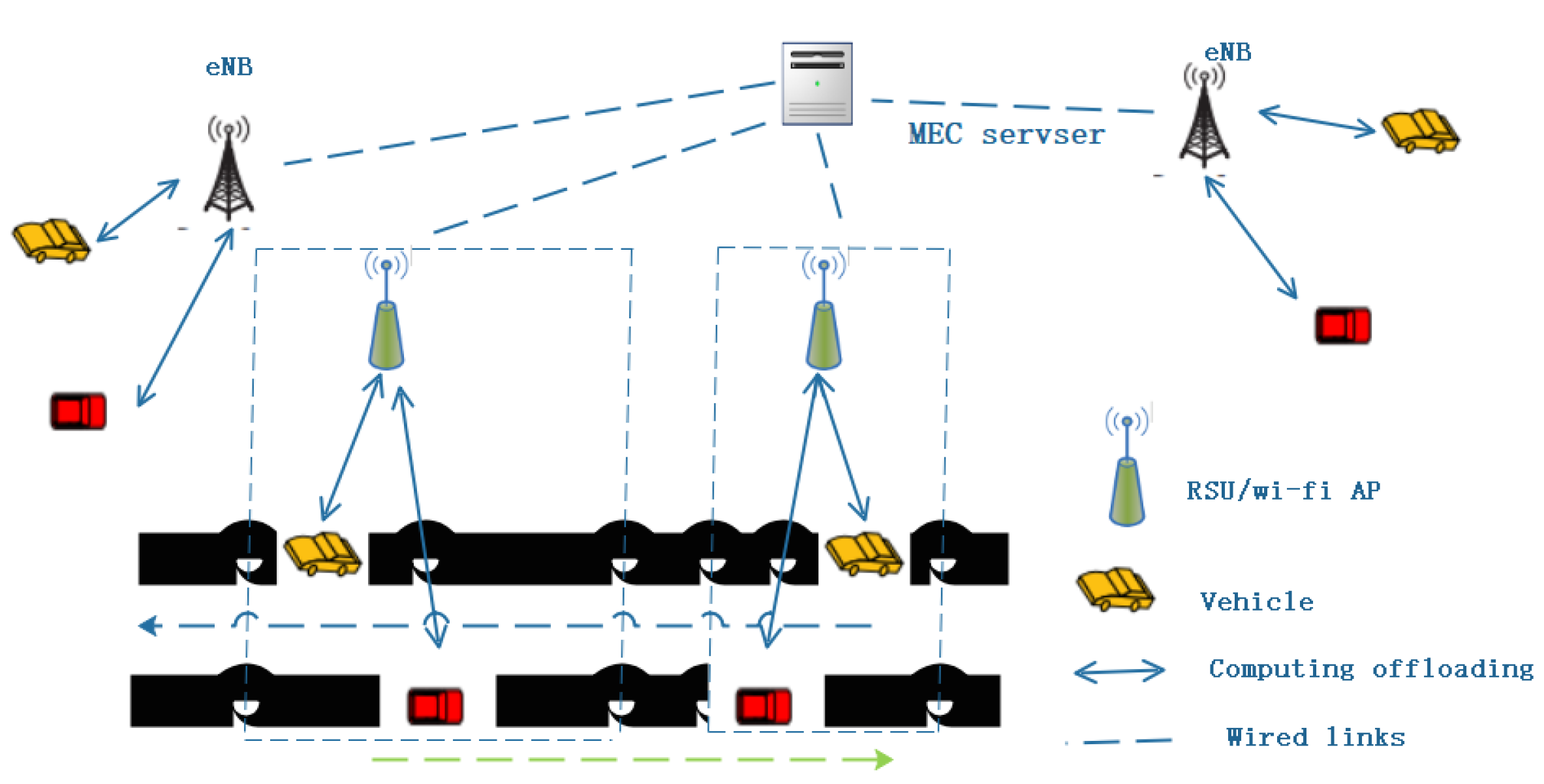
In this section, we discuss some models and special concept definitions (
Figure 1).
A VNET consists of multiple eNBs, multiple RSUs that host the MEC server and multiple vehicles. The MEC server is placed around the edge of the core network rather than eNBS, which allows vehicles to access computing source via different wireless access methods. We suppose that the requesting vehicle is able to simultaneously offload the computing task and upload its tasks to the RSU by using a full-duplex technology [
28,
29]. We apply a MEC-based VNET to sustain multi-vehicles. Many vehicles in the vicinity of several eNBS coverage are served by the same MEC server, and expanding the range of MEC services can meet the challenges of high-speed mobile vehicles better. The eNBs that connect the entire coverage area of the MEC server are defined as the service areas of the server. To achieve resource utilization and ensure minimal VNET network loss, we consider a reasonable scheduling strategy to adjust computing tasks to different requesting vehicles and coordinate wireless access for vehicles through a wide range of resources. Here, multi-vehicles are treated as multi-task, when multiple vehicles are performing computation task offloading, there will be some impacts such as delay time and load balancing indicators on overall VNET. We need to apply the best scheduling strategy to minimize VNET loss. To avoid conflicts between multiple computing tasks when the vehicle moves, we use a multi-task scheduling (MTS) algorithm to minimize the loss of the overall network performance. Next, in the multi-task scheduling process, we model multi-task scheduling as a multi-objective optimization problem, and then try to find this Pareto optimal solution. Below, we give the specific parameters and model design.
Let be the set of N computation tasks. Now, we consider the multi-task scheduling problem over a task space and a set of state space . To enable a large set of training sets, is given, where M is the number of input data points, N is the number of computing task, and is the state of the jth task for ith input data point.
We observe a hypothesis function with respect to each task by , where parameters are shared between primary task and some special tasks . We define the loss function for the special task as: .
Although many loss functions and hypothesis functions have been mentioned in the general machine learning literature, they in general have the following objective form:
where
is the weight of each task, and
is the empirical loss function of the task
j:
.
Although the weighted cumulative sum function seems attractive, it usually either obtains an expensive search or a heuristic using various scales [
30,
31]. The fundamental reason for scaling is the inability to define local optimality in MTS scenarios. Let us define two sets of solutions
and
to enable that
and
, with respect to tasks
and
. That is, the solution of
is better for task
while
is favored by
.
On the other hand, MTS can be modeled as MOO: optimizing a set of objectives that may cause conflicts. We define the MOO function of MTS with a vector of loss function:
The goal of MOO is to obtain the Pareto optimal solution.
The Pareto optimality of MTS is as follows:
- (1)
A solution decides a solution if and only if and .
- (2)
If no solution dominates , then solution is called the Pareto optimal solution.
In the paper, we investigate multi-gradient descent algorithm to solve multi-objective optimization problems.
4. Multi-Objective Optimization Solution
Multi-objective optimization can solve the local optimal solution by gradient descent. In this section, we summarize a multi-gradient descent algorithm (MGDA) to solve it. MGDA makes good use of the KKT conditions necessary for optimization [
24,
32]. We now describe the KKT condition for the shared parameters of the primary task and the special task:
We first give the definition of KKT: the solution of general nonlinear programming problem must satisfy Karush–Kuhn–Tucker (KKT) conditions, provided that the problem constraints satisfy a regularity condition called constraint qualification. If the problem is comprised of a convex set of constraints (i.e., the solution space is convex), and the maximal value (maximal value) of objective function is concave (convex), KKT conditions are sufficient. By applying KKT condition to linear programming, we can obtain the complementary slackness conditions of primal problem and its dual problem.
4.1. Pareto-Stationarity
Let
be a convex function over the open ball
centered at the shared parameter
. These functions are called Pareto optimal for the
point if and only if there is a convex combination of gradient vectors
, in which ∇ denotes the symbol of the gradient that is equal to zero:
Thus, any solution that satisfies the condition in Equation (
3) is denoted as the Pareto stable point. Each Pareto optimal is Pareto stable, and vice versa. Consider the following optimization problem:
It means that either the solution to the optimization problem is equal to zero and the KKT condition is satisfied, or the solution solves the gradient descent direction for improving all tasks. Therefore, MTS algorithm will become a gradient reduction by solving Equation (
4) on a specific task parameter and applying its solution
to the gradient update of the shared parameters. We consider how to solve Equation (
4) for any model in
Section 4.2 and propose an effective solution when the base model is a shared-special case in
Section 4.3.
4.2. Handling the Optimal Solution
The optimal problem defined in Equation (
4) is equal to seeking a minimal norm weight point in the convex hull of an input parameter space. This was originally generated in computational geometry: that is, to find a point in the convex hull that is the closest to a given query point. They have been extensively studied [
33,
34,
35], and even though many researchers have proposed algorithms to solve the issue, they are not fit for our problem, because the assumptions under these algorithms are too ideal. Although some algorithms have solved the problem of finding the minimum norm in convex hulls that are composed of a large number of points of low dimensional space (usually dimension 2 or 3), under our assumption, the number of points in input parameter equals the number of tasks in the system, which is generally low. In comparison, the dimensionality, i.e., the number of shared parameters, is considered high. We therefore use a convex optimization method to solve it, because Equation (
4) is also a linearly constrained convex quadratic function.
Before we solve this problem, we first consider the general situation of a two-task. The problem is formulated as .
We first show the minimum norm point in a convex hull of two input points, i.e., . The Algorithm is given below:
| Algorithm 1: |
1: if then
2:
3: else if then
4:
5: else
6:
7: end if |
Although this only applies to the case of the number of tasks
, since the linear search can be analytically solved, this enables the Frank-Wolfe Algorithm [
36] to be applied as well, thus we use it to solve the optimization constraint problem and obtain a solution:
Using the Equation (
5) as a step for linear search, we obtain the update of the Frank-Wolfe Algorithm [
36] as follows.
| Algorithm 2: Update Algorithm for MTS |
1: for to N do
2:
3: end for
4:
5:
6: Perform Frank–Wolfe Algorithm
7: Initialize
8: Computer V s.t
9: repeat
10:
11:
12:
13: until or Iteration Step Limit
14: return
15: end perform |
4.3. Reasonable Optimization of Gradient Computation
The MTS update algorithm in Algorithm 2 is suitable for any gradient descent based optimization problem. The experimental results also show that the Frank–Wolfe algorithm is accurate and efficient because it usually converges within a moderate number of iterations and the impact on the training set is negligible. However, our proposed algorithm needs to compute for every task j, a step that needs a backward propagation through shared parameters. Therefore, the resulted gradient computation will be forward propagation following N backward propagation. Since backward propagation is generally more expensive than forward propagation, the linear scaling of training time is a prohibition for many tasks.
We provide an effective way for optimizing the MTS objective and only need one post-propagation. We also show that the upper bound can produce a Pareto optimal solution under the assumption of reality. We define a shared representation function with a special task decision function that covers many existing deep multi-learning models and can also be denoted by constraining hypothesis class:
where
r is the all tasks’ representation function, and
is the specific task function that takes these representation functions as input. Now, we define the representation function as
,
and we can directly express the upper bound as:
where
is the Jacobian matrix form of
A with respect to
. The upper bound has two properties described below: (1)
is computed for all tasks in the form of a single backward propagation; and (2)
is not a function
, thus it can be cancelled when it is used as an optimization objective. We use the upper bound to replace the term
. We derive the approximate optimization by throwing the
term that does not affect this optimization, so the optimization result is:
We call this problem a multi-gradient descent algorithm based on upper bound (MGDA-UB). In fact, MGDN-UB corresponds to the gradient using the task loss for the representation rather than sharing parameters. We only changed the last step of Algorithm 2.
Although the MGDA-UB is close to the original optimization algorithm, we describe it in a theorem to demonstrate the fact that our proposed algorithm yields a Pareto optimal solution under original hypothesis. Please see the proof in
Appendix A.
Theorem 1. If is the solution of MGDA-UB and assuming is full rank, then one of the following is true:
- (i)
and the existing parameters are Pareto stationary.
- (ii)
is a descent direction which decreases every objective value.
This conclusion results by a fact that, as long as is full rank, the upper bound corresponding to minimizing the convex combination norm gradient defined by using the Mahalonobis norm is optimized. This non-singular hypothesis is true because singularity means tasks are linearly related and do not need a trade-off. Overall, our proposed algorithm can find a Pareto optimal stable point with almost negligible computational cost and apply it to any MTS problem using a shared-special model.
5. Experimental Results
1. An MTS adaptation of the MNIST dataset
We evaluated the proposed MTS algorithm on the MultiMNIST dataset. Our algorithm’s evaluation was based on the following three indicators as the benchmark:
- (1)
Uniform scaling: Minimizing the uniformly weight sum of the loss function i.e., .
- (2)
Single task: Solving tasks individually.
- (3)
Grid search: Exhaustively searching for different values from and minimizing .
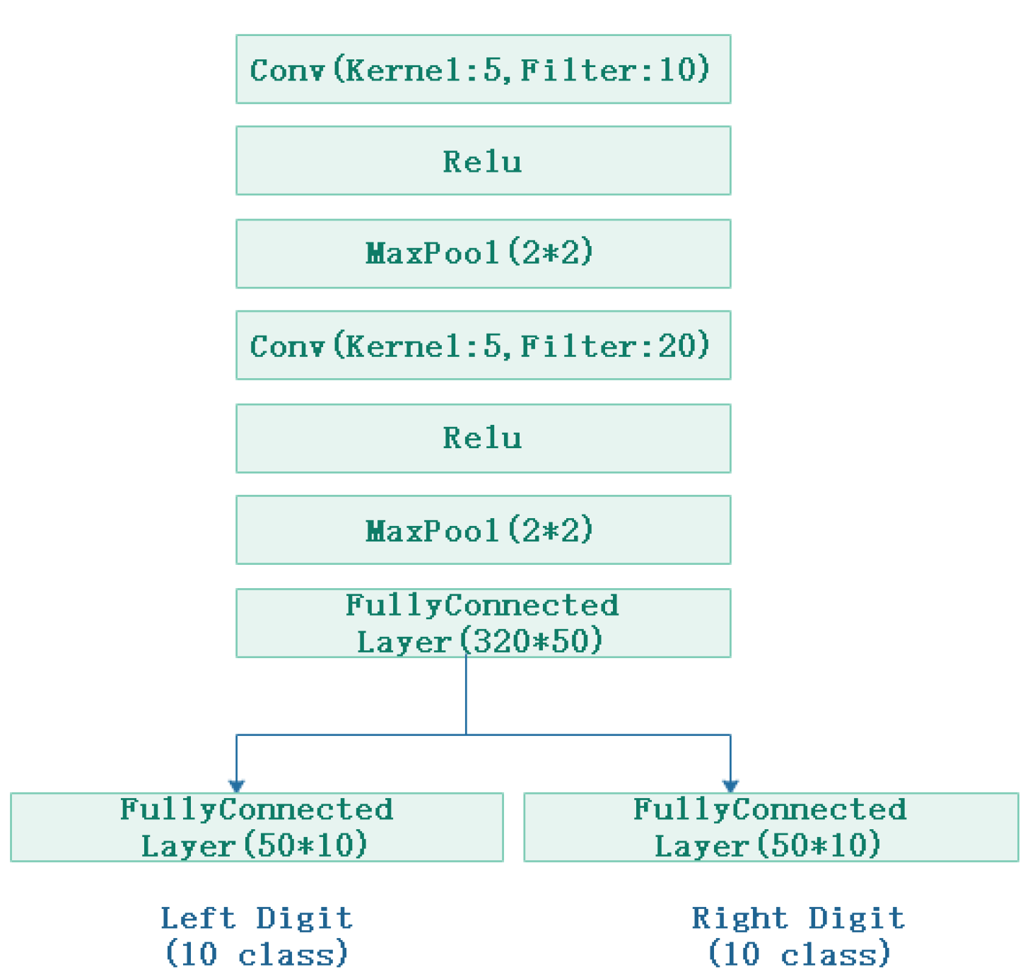
To convert data classification into MTL problem, Sabour et al. stacked a large amount of images together. We used the same structure. For each image, we randomly selected a different image, and then placed one of these images on the upper left and the rest on the bottom right. The result is as follows: classify the data in the upper left and classify the data in the upper right. The 60 k example was used here and the existing single-task MNIST model was used directly. For the MultiMNIST experiment, we used the LeNet structure [
37]. We used all layers (except last layer) as a representation function (or a shared coder). By simply adding two fully connected layers, we could treat the fully connected layer as a function of the task-special for all tasks, and each output of the representation function was taken as an input.As a loss function for a task-special, we used a softmax cross-entropy loss for both tasks.
Figure 2 shows the structure.
We used PyTorch to do the experiment [
38]. The learning rate was set as
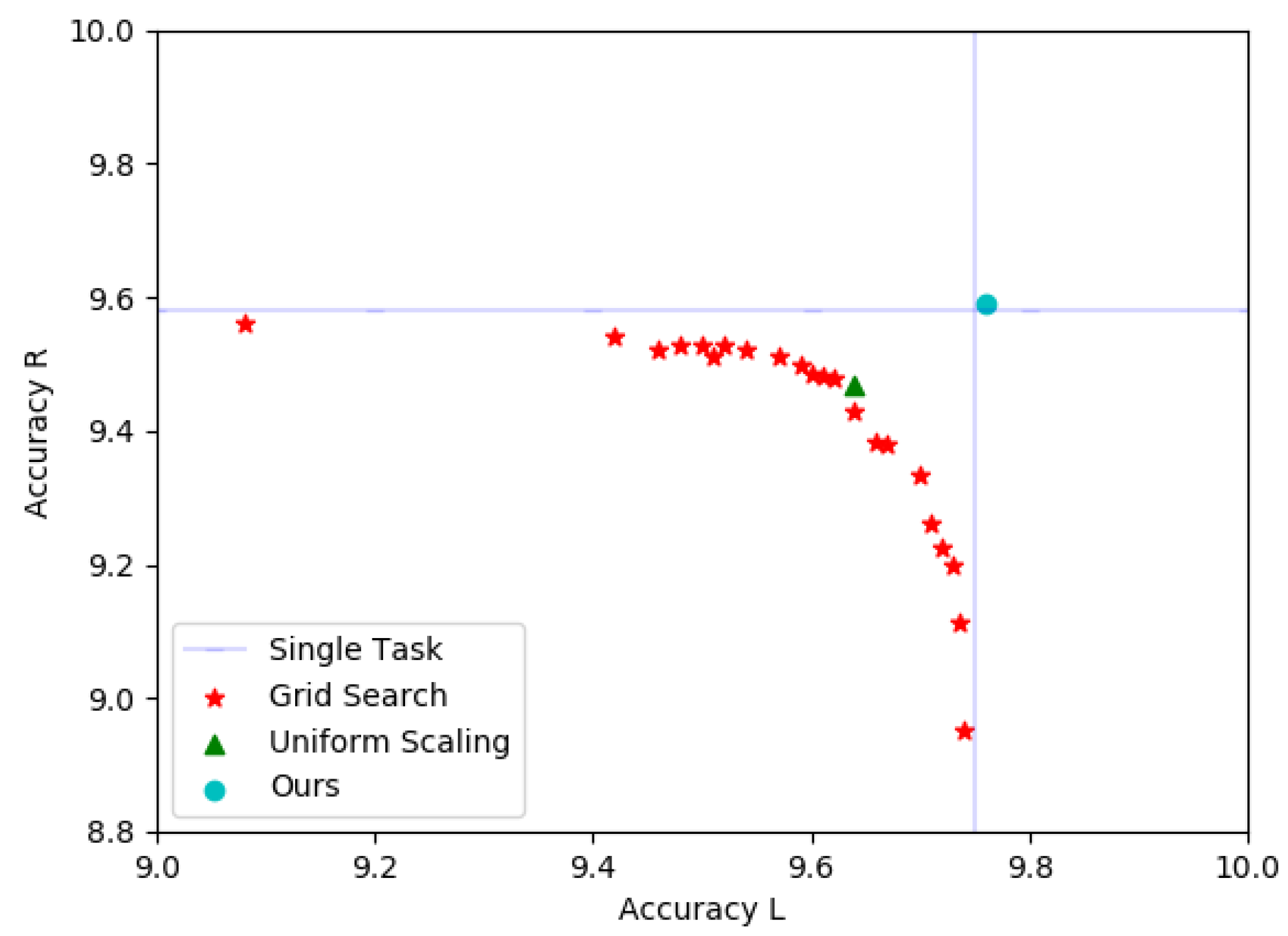
, and we selected the model’s learning rate that produced the highest validation correctness. We used momentum SGD. We halved the learning rate for every 20 generations, and we trained 50 times with the batch size 128. We describe the performance graph as a scatter plot of the accuracy of Task-L and Task-R in
Figure 3. Our scatter plot describes the accuracy of detecting the left and right digits of all baselines. This grid shows the capacity of the computing task to compete for the system model. Our approach is the only one that embodies a solution that is as good as training a dedicated model for each computing task and is better at the top right.
Table 1 shows the performance of the MTS algorithm on MultiMNIST. The single task basis can solve a single task independently with a dedicated model. The results also show that our method can find a solution that can produce as accurate solution as the single task solution. It also shows that the effectiveness of our method is as good at MTS as MOO.
2. Scenario realization
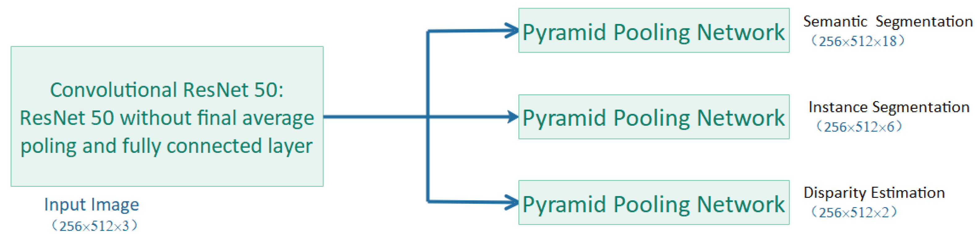
We used GRB images to implement a more realistic scene. We dealt with three tasks: instance segmentation, semantic segmentation, and monocular depth segmentation. We used a shared-special task structure. The shared task mode was based on the full convolutional form of ResNet-50 architecture [
39]. We only used the layer that is better than the average pool with full convolutions. For the special task form, we used the pyramid pooling module [
40] and assigned the output scale to
for semantic segmentation,
for instance segmentation, and
for monocular depth segmentation. For the loss function, we used the cross entropy with the softmax function as the semantic segmentation, the MES for the depth and instance segmentation, as shown in
Figure 4.
We used pre-training on ImageNet [
41] to initialize the shared task model. We applied an application of diamond pool network with bilinear interpolation that was also used by Zhou et al. [
42]. Cityscapes measure set are usually not available. Thus, we used a verification set as the report result. For a validation set with hyperparametric search target, we randomly selected 260 images in the training targets. When choosing optimal hyperparameters, we used the full training target set to do retraining, kept our algorithm hidden during training and hyperparameter search, and reported measure results on Cityscapes validation set. For semantic segmentation, we measured it by mean intersection over union, and for instance segmentation we used MES. For semantic segmentation, we did not perform the cluster operation further, but reported the test results directly in the proxy task. In our experiment, we searched through the learning rate set
and selected the model with the highest verification accuracy. We halved the learning rate for every 20 epochs, and we trained 200 times with the batch size 8.
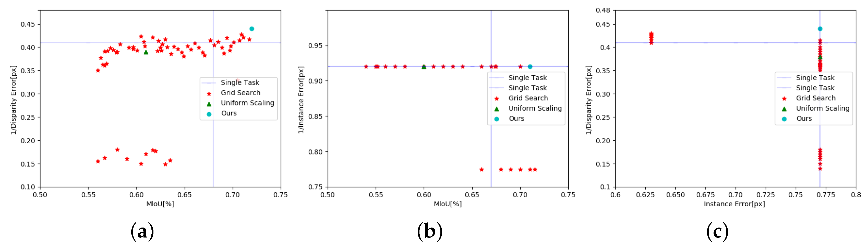
Figure 5a–c shows the performance of all baselines for semantic segmentation tasks, instance segmentation tasks, and monocular depth segmentation tasks, respectively. We used each pixel regression error to represent instance segmentation, mIoU for semantic segmentation, and disparity error for monocular depth segmentation. To convert errors of measure performance, we used 1/disparity error. We drew a two-dimensional project that represents the performance profile for each pair of computing tasks. Although we drew pairwise project for expressing visual effects, each point in the graph solves all computing tasks, and the top right is better.
Table 2 shows the performance of MTS performance in three different instances. It also displays each task pair’s performance, even though we performed all tasks simultaneously on three baselines.
6. Conclusions
In this paper, we form a framework of optimal resource allocation strategy for computing in vehicular networks. We formulate the optimal computing task scheduling to minimize the VNET loss under the constraints of dynamically computational resource at RSU and the limited storage capacities as well as under the constraints of hardware deadline at end-to-end and the vehicular mobility. To avoid conflicts between tasks during vehicle mobility, we convert the multi-task scheduling problem into a multi-objective optimization problem, and then find the Pareto optimal solution. For the specific large-scale vehicular network in reality, we propose a Frank–Wolfe–based MGDA optimization algorithm and extend it to the high-dimensional space. Meanwhile, we give the upper bound of the MGDA algorithm and prove it can be solved by a backward propagation without a specific-task gradient. Finally, the experimental results show that our method is greatly improved in terms of accuracy compared with the existing methods.
7. Future Works
In this paper, we study how to implement an effective and reasonable scheduling strategy in the vehicular network to minimize the performance loss of the entire network. The significance of this research is that classification-based tasks have been well promoted in the field of deep learning models, but there are certain limitations. For example, as the size of the network increases and the number of vehicles increases, there will be phenomena such as traffic congestion and insufficient cache. How to solve these problems in the super network will be considered in the future. At the same time, in the vehicular network, when the vehicle moves on the roadside base unit, privacy information will be revealed. How to design the encryption scheme will also be considered in the future.
Author Contributions
Conceptualization, methodology, and validation, X.Z., Y.C. and M.L.; Investigation and visualization, X.Z., Y.C., M.L.and J.G.; Writing—original draft preparation, X.Z., Y.C. and M.A.; Writing—review and editing, and supervision, X.Z., Y.C., J.G. and M.A.; and Funding acquisition, M.L. and Y.C.
Funding
This work was supported by the National Natural Science Foundation of China (Grant Nos. 61572095, 61877007, and 61802097), and the Project of Qianjiang Talent (Grant No. QJD1802020).
Acknowledgments
Thanks to the reviewers and editors for their careful review, constructive comments, and English editing, which helped improve the quality of the paper.
Conflicts of Interest
The authors declare no conflict of interest.
Appendix A
Proof of Theorem 1. The first case: If MGDA-UB’s optimal value is 0, then that of Equation (
3) is as well. We now consider the second case: if the optimal value of MGDA-UB is 0, the value of Equation (
3) is not 0:
Here,
is the solution of Equation (
4) and the optimal value of Equation (
4) is 0. This gives proof of the first case. Before we start the second case, let us give a lemma first. Since
is full rank, this equivalence is two-way. That is, if
is the solution of Equation (
4), then it is also the solution of the MGDA-UB. Thus, both formulas follow Pareto stability.
We need to prove that the descent direction obtained by computing (MGDA-UB) does not increase the value of loss functions in order to prove the second case. The formal expression is given below:
This condition is equivalent to the following:
where
; since
M is positive definition, this is further equivalent to the following:
We prove that this is derived from the (MGDA-UB) optimality condition. The Lagrange of MGDA-UB is expressed as:
Lagrange’s KKT conditions yield the expected results as follows:
☐
References
- Chen, Y.; Wang, L.; Ai, Y.; Jiao, B.; Hanzo, L. Performance analysis of NOMA-SM in vehicle-to-vehicle massive MIMO channels. IEEE J. Sel. Areas Commun. 2017, 35, 2653–2666. [Google Scholar] [CrossRef]
- Wang, J.; Jiang, C.; Han, Z.; Ren, Y.; Hanzo, L. Internet of vehicles: Sensing-aided transportation information collection and diffusion. IEEE Trans. Veh. Technol. 2018, 67, 3813–3825. [Google Scholar] [CrossRef]
- Ahmed, E.; Gani, A.; Sookhak, M.; Ab Hamid, S.H.; Xia, F. Application optimization in mobile cloud computing: Motivation, taxonomies, and open challenges. J. Netw. Comput. Appl. 2015, 52, 52–68. [Google Scholar] [CrossRef]
- Taleb, T.; Dutta, S.; Ksentini, A.; Iqbal, M.; Flinck, H. Mobile edge computing potential in making cities smarter. IEEE Commun. Mag. 2017, 55, 38–43. [Google Scholar] [CrossRef]
- Dinh, H.T.; Lee, C.; Niyato, D.; Wang, P. A survey of mobile cloud computing: Architecture, applications, and approaches. Wirel. Commun. Mob. Comput. 2013, 13, 1587–1611. [Google Scholar] [CrossRef]
- Liu, J.; Ahmed, E.; Shiraz, M.; Gani, A.; Buyya, R.; Qureshi, A. Application partitioning algorithms in mobile cloud computing: Taxonomy, review and future directions. J. Netw. Comput. Appl. 2015, 48, 99–117. [Google Scholar] [CrossRef]
- Cloud, A.E.C. Amazon web services. Retrieved November 2011, 9, 2011. [Google Scholar]
- Chen, Y.; Zhang, Y.; Maharjan, S.; Alam, M.; Wu, T. Deep Learning for Secure Mobile Edge Computing in Cyber-Physical Transportation Systems. IEEE Netw. 2019, 33, 36–41. [Google Scholar] [CrossRef]
- Chen, Y.; Guizani, M.; Zhang, Y.; Wang, L.; Crespi, N.; Lee, G.M.; Wu, T. When Traffic Flow Prediction and Wireless Big Data Analytics Meet. IEEE Netw. 2019, 33, 161–167. [Google Scholar] [CrossRef]
- Mach, P.; Becvar, Z. Mobile edge computing: A survey on architecture and computation offloading. IEEE Commun. Surv. Tutor. 2017, 19, 1628–1656. [Google Scholar] [CrossRef]
- Shi, W.; Cao, J.; Zhang, Q.; Li, Y.; Xu, L. Edge computing: Vision and challenges. IEEE Internet Things J. 2016, 3, 637–646. [Google Scholar] [CrossRef]
- Patel, M.; Naughton, B.; Chan, C.; Sprecher, N.; Abeta, S.; Neal, A. Mobile-Edge Computing Introductory Technical White Paper. White Paper, Mobile-Edge Computing (MEC) Industry Initiative. 2014. Available online: https://portal.etsi.org/portals/0/tbpages/mec/docs/mobile-edge_computing_-_introductory_technical_white_paper_v1%2018-09-14.pdf (accessed on 7 August 2019).
- Ahmed, E.; Rehmani, M.H. Mobile edge computing: Opportunities, solutions, and challenges. Future Gener. Comput. Syst. 2017, 70, 59–63. [Google Scholar] [CrossRef]
- Désidéri, J.A. Multiple-gradient descent algorithm (MGDA) for multiobjective optimization. C. R. Math. 2012, 350, 313–318. [Google Scholar] [CrossRef]
- Sabour, S.; Frosst, N.; Hinton, G.E. Dynamic routing between capsules. In Proceedings of the Advances in Neural Information Processing Systems, Long Beach, NV, USA, 4–9 December 2017; pp. 3856–3866. [Google Scholar]
- Cordts, M.; Omran, M.; Ramos, S.; Rehfeld, T.; Enzweiler, M.; Benenson, R.; Franke, U.; Roth, S.; Schiele, B. The cityscapes dataset for semantic urban scene understanding. In Proceedings of the IEEE Conference on Computer Vision and Pattern Recognition, Las Vegas, NV, USA, 26–30 June 2016; pp. 3213–3223. [Google Scholar]
- Golrezaei, N.; Molisch, A.F.; Dimakis, A.G.; Caire, G. Femtocaching and device-to-device collaboration: A new architecture for wireless video distribution. arXiv 2012, arXiv:1204.1595. [Google Scholar] [CrossRef]
- Mao, Y.; You, C.; Zhang, J.; Huang, K.; Letaief, K.B. A survey on mobile edge computing: The communication perspective. IEEE Commun. Surv. Tutor. 2017, 19, 2322–2358. [Google Scholar] [CrossRef]
- Xue, Y.; Liao, X.; Carin, L.; Krishnapuram, B. Multi-task learning for classification with dirichlet process priors. J. Mach. Learn. Res. 2007, 8, 35–63. [Google Scholar]
- Argyriou, A.; Evgeniou, T.; Pontil, M. Multi-task feature learning. In Proceedings of the 19th International Conference on Neural Information Processing Systems, Vancouver, BC, Canada, 4–7 December 2006; pp. 41–48. [Google Scholar]
- Ruder, S. An overview of multi-task learning in deep neural networks. arXiv 2017, arXiv:1706.05098. [Google Scholar]
- Misra, I.; Shrivastava, A.; Gupta, A.; Hebert, M. Cross-stitch networks for multi-task learning. In Proceedings of the IEEE Conference on Computer Vision and Pattern Recognition, Las Vegas, NV, USA, 26–30 June 2016; pp. 3994–4003. [Google Scholar]
- Rudd, E.M.; Günther, M.; Boult, T.E. Moon: A mixed objective optimization network for the recognition of facial attributes. In Proceedings of the European Conference on Computer Vision, Amsterdam, The Netherlands, 8–16 October 2016; pp. 19–35. [Google Scholar]
- Schäffler, S.; Schultz, R.; Weinzierl, K. Stochastic method for the solution of unconstrained vector optimization problems. J. Optim. Theory Appl. 2002, 114, 209–222. [Google Scholar] [CrossRef]
- Kuhn, H.W.; Tucker, A.W. Nonlinear programming. In Proceedings of the Second Berkeley Symposium on Mathematical Statistics and Probability, Berkeley, CA, USA, 31 July–12 August 1950; University of California Press: Berkeley, CA, USA; pp. 481–492. [Google Scholar]
- Peitz, S.; Dellnitz, M. Gradient-based multiobjective optimization with uncertainties. In NEO 2016; Springer: Cham, Switzerland, 2018; pp. 159–182. [Google Scholar]
- Poirion, F.; Mercier, Q.; Désidéri, J.A. Descent algorithm for nonsmooth stochastic multiobjective optimization. Comput. Optim. Appl. 2017, 68, 317–331. [Google Scholar] [CrossRef]
- Zhang, Z.; Long, K.; Vasilakos, A.V.; Hanzo, L. Full-duplex wireless communications: Challenges, solutions, and future research directions. Proc. IEEE 2016, 104, 1369–1409. [Google Scholar] [CrossRef]
- Tan, L.T.; Le, L.B. Multi-channel MAC protocol for full-duplex cognitive radio networks with optimized access control and load balancing. In Proceedings of the 2016 IEEE International Conference on Communications (ICC), Kuala Lumpur, Malaysia, 22–27 May 2016; pp. 1–6. [Google Scholar]
- Kendall, A.; Gal, Y.; Cipolla, R. Multi-task learning using uncertainty to weigh losses for scene geometry and semantics. In Proceedings of the IEEE Conference on Computer Vision and Pattern Recognition, Salt Lake City, UT, USA, 18–22 June 2018; pp. 7482–7491. [Google Scholar]
- Chen, Z.; Badrinarayanan, V.; Lee, C.Y.; Rabinovich, A. Gradnorm: Gradient normalization for adaptive loss balancing in deep multitask networks. arXiv 2017, arXiv:1711.02257. [Google Scholar]
- Fliege, J.; Svaiter, B.F. Steepest descent methods for multicriteria optimization. Math. Methods Oper. Res. 2000, 51, 479–494. [Google Scholar] [CrossRef]
- Makimoto, N.; Nakagawa, I.; Tamura, A. An efficient algorithm for finding the minimum norm point in the convex hull of a finite point set in the plane. Oper. Res. Lett. 1994, 16, 33–40. [Google Scholar] [CrossRef]
- Wolfe, P. Finding the nearest point in a polytope. Math. Program. 1976, 11, 128–149. [Google Scholar] [CrossRef]
- Sekitani, K.; Yamamoto, Y. A recursive algorithm for finding the minimum norm point in a polytope and a pair of closest points in two polytopes. Math. Program. 1993, 61, 233–249. [Google Scholar] [CrossRef]
- Jaggi, M. Revisiting Frank-Wolfe: Projection-Free Sparse Convex Optimization. ICML (1). 2013, pp. 427–435. Available online: http://proceedings.mlr.press/v28/jaggi13-supp.pdf (accessed on 7 August 2019).
- LeCun, Y.; Bottou, L.; Bengio, Y.; Haffner, P. Gradient-based learning applied to document recognition. Proc. IEEE 1998, 86, 2278–2324. [Google Scholar] [CrossRef]
- Paszke, A.; Gross, S.; Chintala, S.; Chanan, G.; Yang, E.; DeVito, Z.; Lin, Z.; Desmaison, A.; Antiga, L.; Lerer, A. Automatic Differentiation in Pytorch. NIPS Workshops 2017. Available online: https://openreview.net/forum?id=BJJsrmfCZ (accessed on 7 August 2019).
- He, K.; Zhang, X.; Ren, S.; Sun, J. Deep residual learning for image recognition. In Proceedings of the IEEE Conference on Computer Vision and Pattern Recognition, Las Vegas, NV, USA, 26–30 June 2016; pp. 770–778. [Google Scholar]
- Zhao, H.; Shi, J.; Qi, X.; Wang, X.; Jia, J. Pyramid scene parsing network. In Proceedings of the IEEE Conference on Computer Vision and Pattern Recognition, Honolulu, HI, USA, 21–26 July 2017; pp. 2881–2890. [Google Scholar]
- Deng, J.; Dong, W.; Socher, R.; Li, L.J.; Li, K.; Fei-Fei, L. Imagenet: A large-scale hierarchical image database. In Proceedings of the 2009 IEEE Conference on Computer Vision and Pattern Recognition, Miami, FL, USA, 20–26 June 2009; pp. 248–255. [Google Scholar]
- Zhou, B.; Zhao, H.; Puig, X.; Fidler, S.; Barriuso, A.; Torralba, A. Scene parsing through ade20k dataset. In Proceedings of the IEEE Conference on Computer Vision and Pattern Recognition, Honolulu, HI, USA, 21–26 July 2017; pp. 633–641. [Google Scholar]
© 2019 by the authors. Licensee MDPI, Basel, Switzerland. This article is an open access article distributed under the terms and conditions of the Creative Commons Attribution (CC BY) license (http://creativecommons.org/licenses/by/4.0/).


