Abstract
Tourism forecasting is a significant tool/attribute in tourist industry in order to provide for careful planning and management of tourism resources. Although accurate tourist volume prediction is a very challenging task, reliable and precise predictions offer the opportunity of gaining major profits. Thus, the development and implementation of more sophisticated and advanced machine learning algorithms can be beneficial for the tourism forecasting industry. In this work, we explore the prediction performance of Weight Constrained Neural Networks (WCNNs) for forecasting tourist arrivals in Greece. WCNNs constitute a new machine learning prediction model that is characterized by the application of box-constraints on the weights of the network. Our experimental results indicate that WCNNs outperform classical neural networks and the state-of-the-art regression models: support vector regression, k-nearest neighbor regression, radial basis function neural network, M5 decision tree and Gaussian processes.
1. Introduction
During the last decades, tourism has been developed into one of the fastest growing industries worldwide; thus, it constitutes a significant factor of the economic growth of a country. In general, the volume of tourism affects all tourism associated businesses in a country, thus affecting positively the total economy of the country. For example, the economic state and growth of airline companies, hotels, restaurants, market-places and so on are directly affected by tourism volume. According to the Greek Tourism Confederation’s latest report [1], in 2017, tourism industry was boosted to almost 27.2 million tourists and generated a total of 14.2 billion euros for Greek economy. As a result, tourism’s direct contribution to Greece’s GDP increased from 16.7% to 18.3%.
Businesses and tourist organizations, to be viable, need careful management and planning. Therefore, forecasting tourism volume is of significant importance for the effective planning and implementation of tourism strategies (see [2,3,4,5,6] and the references therein). Flight scheduling, hotel and room availability, management of staffing and capacity, and financial viability for implementing a tourism project are just some examples in which tourism demand forecasting is considered essential. As a result, there is an increasing interest for more accurate predictions of tourism volume and demand together with the development of more advanced forecasting techniques.
For the problem of forecasting tourism volume and demand, several methodologies have been applied and proposed, covering a broad range of different methods which can be divided into two main categories: time-series methods and machine learning methods.
Time-series methods constitute the traditional way for monitoring and forecasting tourist volume while AutoRegressive Integrated Moving Average (ARIMA) and its variations are probably the most widely used time-series forecasting models, which has been applied in a variety of real-world tourism data. Kul and Witt [7] conducted a comprehensive comparison of the error correction model, ARIMA and various structural time-series models and found that relative forecasting performance is heavily dependent on the value of forecasting horizon. Song and Li [8] performed an exhaustive review on forecasting time-series of tourism demand. From their findings, they concluded that there is no single model which can exhibit the best forecasting performance and accuracy, in all situations.
Nevertheless, the main disadvantage of time-series methods is that they require assumptions such as stationarity or distribution; thus, they cannot depict the nonlinear and stochastic nature of tourism flow. Therefore, machine learning models have emerged leading to more accurate and efficient forecasting models [9,10,11]. The characteristics of these models, such as adaptability and nonlinearity, make them very useful on tourism forecasting tasks providing an alternative approach to the classical regression time-series models. Artificial Neural Networks (ANNs) are widely accepted as probably the most dominant machine learning models which have been found to be more accurate than other prediction models [12,13]. Due to their self-learning capability and their universal approximation ability, they can efficiently capture the nonlinearity of samples in the data; thus, they have been successfully applied in order to gain a more meticulous view of tourism forecasting.
In this work, we develop a new time-series model based on Weight-Constrained Neural Networks (WCNNs) for forecasting tourist arrivals, which constitutes the contribution of this work. WCNNs constitute a new type of ANNs, which are characterized by imposing bounds on the weights of the network. We conducted a series of experiments and compared the forecasting performance of these new forecasting models against classical ANNs as well as other state-of-the-art regression models. For these experiments, we utilized official statistical data from the Hellenic Statistical Authority regarding domestic and foreign tourists arrivals in Greek hotels from 2004 to 2017. The reported numerical experiments illustrate the prediction accuracy of WCNNs, providing empirical evidence that imposing box-constraints on the weights benefits the prediction performance of the network.
The remainder of the paper is organized as follows: Section 2 presents a survey of recent studies regarding the application of machine learning in forecasting tourist volume and demand. Section 3 presents a brief description of the weight-constrained networks. Section 4 presents the datasets used in our study and Section 5 presents the numerical experiments. Finally, Section 6 presents the conclusions of the paper and outlines its future prospects.
2. Related Work
The increasing development of social economy and the significant improvement of people’s living standard lead to the establishment of tourism as a rapidly growing economic industry. The tourism expenditure has been transformed as a significant source of economic profit, thus an increasing need for accurate forecasting of tourism volume, flow and demand has been generated to reduce risk and uncertainty. Nevertheless, the accurate prediction of tourism flow is considered as one of the most challenging tasks in the intelligent tourism decision system, and mostly in the short-term forecast. Therefore, a number of prediction models based on machine learning techniques have been proposed in the literature to improve the forecasting. In recent years, several studies have been conducted and some useful findings and conclusions are briefly presented below.
Kamel et al. [14] conducted a performance evaluation of seven machine learning methods, namely MultiLayer Perceptron (MLP), k-Nearest Neighbor Regression (kNN), Generalized Regression Neural Network (GRNN), Radial Basis Function Neural Network (RBF), Support Vector Regression (SVR)Classification, and Regression Trees (CART) and Gaussian Processes (GP), to forecast tourism demand to Hong Kong. Their experimental results show that the generalized regression neural network slightly outperformed the other regressors. Nevertheless, the authors concluded that no single method can be considered the best one for all the datasets.
Chen [15] forecasted tourism demand time-series data with possibly nonlinear characteristics by hybridizing linear and nonlinear statistical models. The motivation of the combined model is based on fact that no single method exhibiting the best performance in handling time-series generated from both linear and nonlinear underlying processes exists. The reported numerical results on several test cases of tourism demand time-series reveal that the proposed ensemble models are superior to the single models. Based on the experimental analysis, the author claimed that the proposed combination methodology can achieve considerably better forecasting performance.
Peng and Lai [16] evaluated the performance and effectiveness of tourism e-commerce service innovation utilizing a new framework based on an ANN model. Initially, they proposed an evaluation index system that is consistent with the characteristics of the tourism e-commerce service industry. This system overcomes the difficulty of the ambiguity of the evaluation, rendering detailed measurement indicators for e-commerce service providers. Additionally, they conducted an empirical analysis to measure the performance of their proposed methodology by utilizing an ANN based on ten selected tourism e-commerce service providers. Finally, the authors highlighted the effectiveness and feasibility of the neural networks in evaluating online service innovation and expressed their expectation that the proposed methodology could be used as a reference for future e-commerce service industry innovation evaluations.
Claveria and Torra [11] compared the forecasting performance of ANNs against different time-series models at a regional level utilizing different forecast horizons (1, 2, 3, 6 and 12 months). They collected data from the Statistical Institute of Catalonia and the Direcció General de Turisme de Catalunya concerning monthly tourist arrivals and accommodations from foreign countries to Catalonia covering the time period between 2001 and 2009. Their findings reveal that the ARIMA models surprisingly outperformed ANN models, obtaining more accurate forecasts, especially for shorter forecasting horizons. The authors claimed that the reason for this is that the application of a filtering process and the elimination of the existing outliers as a data preprocessing step lowers the performance of ANNs. Additionally, their presented results show that the performance of ANN models could be significantly improved through structure and hyper-parameter optimization.
Along this line, Claveria et al. [9] compared and evaluated the performance of three different ANNs models for tourist demand forecasting: Elman recursive Neural Network (ERNN), RBF and MLP. The main goal of their research was to improve forecasting performance on tourism demand by utilizing ANN models with different architectures and ways of handling the input information. Thus, they performed several experiments assuming several neural network topologies as well as lags to examine their effects on the forecasting results. Based on their experimental analysis, the authors concluded that MLP and RBF exhibited better forecasting performance than ERNN. Additionally, they also claimed that the increase in the dimensionality, obtained for longer forecasting horizons, can improve the forecasting performance for long-term forecasting.
3. Weight-Constrained Neural Networks
WCNNs constitute a new type of ANNs that are characterized by the application of conditions on the weights of the neural network by means of box-constraints. The rationale of this strategy is focused on defining the weights in the trained network in a more uniform way, by restricting them to take values within pre-defined intervals.
More specifically, as highlighted by Reed and Marks [17], “large weights tend to cause sharp transitions in the node functions”. In such case, it is likely that the network has learned the statistical noise in the training set causing overfitting, which makes the network unstable [18]. This instability with respect to the training data makes the prediction model unreliable since minor variations or uncertainties on the expected inputs may be greatly magnified and lead to wildly different responses. As a result, the network will exhibit poor prediction performance on new unseen data. On the other hand, small weights suggest a less complex and, in turn, more stable prediction model that is less sensitive to statistical fluctuations in the inputs and less likely to overfit the training data [18].
Taking into account the above consideration, we recall that WCNNs eliminate the likelihood that the weights can “blow up” to unrealistically large values by placing box-constraints on the weights. Furthermore, these new prediction models have been empirically proven by numerical experiments in a variety of real-world problems [19,20,21] to present better generalization ability compared to classical ANNs.
The problem of training a WCNN is mathematically formulated as a constrained optimization problem, namely
with
where is the error function and and denote the vectors with the lower and upper bounds on the weights, respectively. An overview of a WCNN is demonstrated in Figure 1.
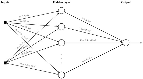
Figure 1.
Typical example of a weight-constrained neural network with a single hidden layer.
For efficiently training a WCNN, Livieris [19] proposed a training algorithm which utilizes a gradient-projection strategy to handle the bounds on the weights by determining an active set corresponding to those weights which are on either their lower or upper bounds. For efficiently minimizing the error function in Equation (1), the proposed training algorithm takes advantages of the numerical efficiency of the L-BFGS (Limited-memory Broyden–Fletcher–Goldfarb–Shanno) matrices.
Adaptive Nonmonotone Active Set-Weight Constrained-Neural Network Training Algorithm
Motivated by the previous work, Livieris and Pintelas [22] proposed an Adaptive nonmonotone Active set -weight-constrained- Neural Network (AANN) training algorithm. This algorithm is based on a conjugate gradient philosophy and it consists of two distinct phases: the gradient projection phase and the unconstrained optimization phase.
The first phase utilizes an adaptive Nonmonotone Gradient Projection Algorithm (aNGPA), which utilizes the property of an active-set estimate to identify the active constraints, ensuring a considerable reduction in the error function in Equation (1). At each iteration, aNGPA initially calculates the search direction
where is the current iterate, , P denotes the projection onto the feasible set and is the sage-guarded Cyclic Barzilai and Borwein stepsize [23]. Subsequently, the procedure utilizes an adaptive strategy based on the concept of the Lipschitz constant to calculate the nonmonotone learning horizon. It is worth noting that the attractive advantage of this strategy is that the utilization of a poorly pre-defined nonmonotone learning horizon is avoided [22]. Then, aNGPA performs a nonmonotone learning search satisfying an Armijo-type condition.
The second phase utilizes a superlinear convergent Conjugate Gradient (CG) algorithm, which is applied in the lower-dimensional space composed by the weights estimated as non-active by aNGPA. The significant advantage of this approach is that the optimization is performed only in the subspace composed of non-active variables, which implies that it allows significant savings in computational time.
Algorithm 1 presents a high level description of the Adaptive nonmonotone Active set-weight constrained- Neural Network (AANN) training algorithm. AANN utilizes algorithm aNGPA to identify the active constraints (face of the feasible set ) and the unconstrained optimization algorithm CG to optimize the error function over a face identified by the aNGPA.
Before presenting the necessary set of rules for switching between the two phases, we give some useful notations. For any , we define the set of active indices, as follows:
Additionally, we define the undecided index set
where and are parameters. Each index corresponds to the component that is not close to zero and the associated gradient component is relatively large. Finally, denotes the vector whose components associated with the set are zero, while the rest of the components are identical to those of .
Initially, algorithm aNGPA is executed until the active constraints satisfying strict complementarity condition are identified, namely in the case and or and . In this case, the training algorithm switches to the CG algorithm, which is applied until a subproblem is efficiently solved. Additionally, when new constraints are identified as active, then algorithm AANN decides to restart either algorithm CG or algorithm aNGPA. Furthermore, another quantity which enters into the switching criteria is relative with the ratio between the norm active gradient components and the error estimator . More specifically, in the case is sufficiently small relative to , the algorithm switches from the unconstrained optimization phase to the gradient projection phase.
Finally, it is worth mentioning that algorithm AANN has complexity and a detailed description of the training algorithm, as well as the procedures of aNGPA and CG, can be found in [22].
| Algorithm 1: AANN | |
| Input: | − Initial weights. |
| − implies the subproblem was efficiently solved. | |
| − Decay factor used to decrease in aNGPA. | |
| − Integer connected with active set repetitions or change. | |
| − Integer connected with active set repetitions or change. | |
| Output: | − Weights of the trained network. |
| Step 1. | repeat |
| Step 2. | Execute aNGPA. /* Phase I: Gradient projection */ |
| Step 3. | if then |
| Step 4. | if then |
| Step 5. | ; |
| Step 6. | else |
| Step 7. | Goto Step 14; |
| Step 8. | end if |
| Step 9. | else if then |
| Step 10. | if then |
| Step 11. | Goto Step 14; |
| Step 12. | end if |
| Step 13. | end if |
| Step 14. | Goto Step 2; |
| Step 15. | Execute CG. /* Phase II: Unconstrained optimization */ |
| Step 16. | if () then |
| Step 17. | Restart aNGPA and goto Step 3; |
| Step 18. | else if () then |
| Step 19. | if ( and ) then |
| Step 20. | Restart aNGPA and goto Step 3; |
| Step 21. | else |
| Step 22. | Restart CG and goto Step 15; |
| Step 23. | end if |
| Step 24. | until (stopping criterion) |
4. Datasets
For the purpose of this research, we used data from January 2004 to December 2017, concerning the domestic and foreign tourists monthly arrivals in Greece. All data were obtained from the official statistical records of the Hellenic Statistical Authority [24].
Figure 2 and Figure 3 illustrate the monthly arrivals of domestic and foreign tourists arrivals in Greece, respectively, from 2004 to 2017. They both present a strong seasonality of 12 months with the maxima of the occupancy arising during the high tourism summer season. The foreign tourists time-series exhibits an increasing behavior throughout summer, while the baseline in the winter remains constant. Regarding the domestic tourists time-series, there exists an increase up to 2009. After the global financial crisis, there is a decrease for about three years and then a borderline increase in the average afterwards.
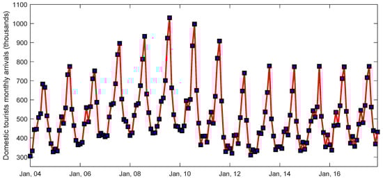
Figure 2.
Monthly arrivals of domestic tourist from 2004 to 2017.

Figure 3.
Monthly arrivals of foreign tourist from 2004 to 2017.
The data from both domestic and foreign tourists monthly arrivals were divided into training set and testing set. The training set consists of data from January 2004 to December 2015 (12 years), which ensures a substantial amount of data for training, as 12 years of tourists’ arrival should cover a wide range of long- and short-term trends. The testing set comprises data from January 2016 to December 2017, which ensures that we forecast the compared prediction models on unseen “out-of-sample” data.
Additionally, both time-series in addition to seasonality show heteroskedasticity, i.e. an unequal variability across the range of values due to the time variations of maxima and/or minima. A common approach in modeling is to utilize the natural logarithms of the series under consideration.
5. Numerical Experiments
We performed an experimental analysis to explore and evaluate the prediction performance of weight-constrained networks in forecasting domestic and foreign tourists arrivals in hotels and compared them against state-of-the-art regression models.
The forecasting performance was evaluated using Root Mean Square Error (RMSE) and Mean Absolute Error (MAE) as performance measures. These metrics have been characterized as probably the most appropriate metric for comparing regression models [25]. RMSE is a quadratic scoring rules which estimates the correctness of the prediction in terms of levels and the deviation between the predicted and the actual values while MAE estimates the average magnitude of the errors in a set of predictions, without considering their direction. They are, respectively, defined by
where n is the number of test instances, and and are the predicted and the actual value for i-instance, respectively. Moreover, the errors were estimated for different values of forecasting horizon, i.e., 6, 9 and 12 months. Forecasting horizon is the number of months for which the arrivals are being taken into consideration for predicting the next month’s arrivals. For example, a forecasting horizon equal to 6 means that the data are being taken for 6 months and results are predicted for the 7th month.
The experimental analysis was conducted by performing a two-phase procedure: In the first phase, we compared the forecasting performance of WCNNs against that of classical ANNs. In the second phase, we evaluated the forecasting performance of the WCNNs against the most popular and frequently used regression algorithms.
5.1. Performance Evaluation of WCNNs Against ANNs
We compared the prediction performance of WCNNs against classical ANNs. For this purpose, we utilized the performance profiles proposed by Dolan and Morè [26] to present perhaps the most complete information in terms of solution quality and efficiency [19,20]. Notice that the performance profile plots the fraction P of simulations for which any given model is within a factor of the best forecasting model. The curves in the following figures have the following meaning:
- “WCNN” stands for a weight-constrained neural network with bounds on all its weights.
- “WCNN” stands for a weight-constrained neural network with bounds on all its weights.
- “WCNN” stands for a weight-constrained neural network with bounds on all its weights.
- “ANN” stands for a classical artificial neural-network.
It is worth mentioning that the weight-constrained networks were trained with AANN algorithm [22] and the classical artificial neural networks were trained with L-BFGS [27]. Notice that both training algorithms were utilized with their default optimized hyperparameter settings.
For forecasting horizons of 6, 9 and 12 months, both WCNNs and ANNs consist of 1 hidden layer with 5, 5 and 6 neurons, respectively. Moreover, the neurons in the hidden layers had logistic activation functions while the ones in the output layer had linear activation functions. Finally, the error goal was set to and the maximum number of epochs was set to 500. The implementation code of all neural networks was written in Matlab 2008a and the simulations were carried out on a laptop (2.4 GHz Quad-Core processor, 4 GB RAM) while the performance was evaluated using the stratified 10-fold cross-validation procedure [28] and the results were obtained over 100 independent simulations.
Figure 4 presents the performance profiles based on RMSE for the domestic tourists arrivals investigating the performance of each forecasting horizon. Firstly, it is worth noting that the weight-constrained neural networks illustrated better regression accuracy than classical neural networks. WCNN1 exhibited the best overall performance, outperforming all forecasting models, followed by WCNN2. More specifically, WCNN1 reported 44%, 43% and 47% of simulations with the best RMSE, for forecasting horizons of 6, 9 and 12 months, respectively, while WCNN2 reported 27%, 27% and 20% and WCNN3 reported 23%, 17% and 26% in the same situations. Furthermore, the ANNs exhibited the worst performance, reporting 7%, 17% and 7% of simulations with the best RMSE, for forecasting horizons of 6, 9 and 12, months respectively.
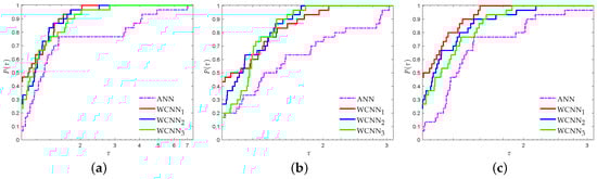
Figure 4.
Performance profiles based on RMSE for domestic tourists arrivals ( scaled). (a) Forecasting horizon = 6; (b) Forecasting horizon = 9; (c) Forecasting horizon = 12.
Figure 5 presents the performance profiles based on MAE metric for the domestic tourists arrivals. WCNN1 presented the lowest MAE score in 37%, 45% and 41% of simulations for forecasting horizons of 6, 9 and 12 months, respectively, while WCNN2 presented 25%, 23% and 23%, WCNN3 presented 27%, 15% and 23% and ANN presented 15%, 20% and 20% in the same situations. Based on the above observations, we can easily conclude that WCNN1 exhibited the best overall performance since its curves lie on the top, regarding all forecasting horizons.
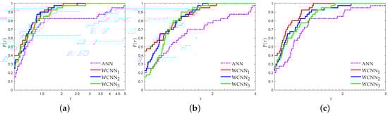
Figure 5.
Performance profiles based on MAE for domestic tourists arrivals ( scaled). (a) Forecasting horizon = 6; (b) Forecasting horizon = 9; (c) Forecasting horizon = 12.
Summarizing, we conclude that imposing box-constraints on the weights of the neural network increased the overall regression accuracy, in most cases. Moreover, tighter bounds are most likely to develop a prediction model with better forecasting performance.
Figure 6 and Figure 7 present the performance profiles for the domestic tourists arrivals based on RMSE and MAE metrics, respectively. Clearly, the interpretation of both Figure 6 and Figure 7 reveals that all versions of WCNNs outperformed ANNs, regarding all forecasting horizons. More specifically, for forecasting horizon of six months, WCNN1, WCNN2 and WCNN3 reported 23%, 28% and 37% of simulation with the best RMSE, respectively, while ANN reported only 13%. For forecasting horizon of nine months, WCNN1, WCNN2 and WCNN3 presented 40%, 33% and 17% of simulation with the best RMSE, respectively, while ANN reported only 10%. Finally, for forecasting horizon of 12 months, WCNN1, WCNN2 and WCNN3 exhibited 23%, 47% and 20% of simulation with the best RMSE, respectively, while ANN reported only 10%. Moreover, relative to the MAE performance metric, WCNN1 and WCNN2 reported the best overall performance since their curves lie on the top, regarding all forecasting horizons.
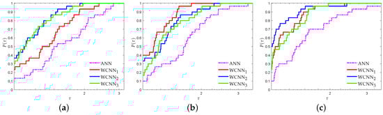
Figure 6.
Performance profiles based on RMSE for foreign tourists arrivals ( scaled). (a) Forecasting horizon = 6; (b) Forecasting horizon = 9; (c) Forecasting horizon = 12.
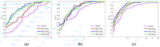
Figure 7.
Performance profiles based on MAE for foreign tourists arrivals ( scaled). (a) Forecasting horizon = 6; (b) Forecasting horizon = 9; (c) Forecasting horizon = 12.
Based on the above numerical experiments, we can easily conclude that the weight-constrained neural networks provided better regression performance than the classical neural networks. Nevertheless, by the comparison of WCNN1, WCNN2 and WCNN3, we can easily conclude that, in case the bounds on the weights are too tight, this may not substantially benefit the forecasting performance.
5.2. Evaluation of WCNNs Against State-of-Art Regression Algorithms
Next, we evaluated the prediction performance of the weight-constrained neural networks against state-of-the-art regression algorithms, namely the Support Vector Regression (SVR), the k-Nearest Neighbor Regression (kNN), the Radial Basis Function neural network (RBF), M5 decision tree and the Gaussian Processes (GP). A brief description of these regression algorithms is presented below:
- SVR [29] is a regression algorithm utilized for predicting continuous output variables instead of classification, for which the classical support vector machines is used. It is based on a different philosophy from other regression models, as it tries to fit the best line within a predefined error value, while other regression models try to minimize the error between the predicted and the actual value.
- kNN [30] is a simple learning method applied to both classification and regression tasks, which utilizes distance functions to measure feature similarity in order to predict the values of any new data point. The final prediction of the kNN regression algorithm is the average value of the closest points to the new point.
- RBF [31] is an ANN which utilizes radial basis functions on all hidden units. Each hidden unit contains a prototype vector and the activation depends on the similarity of the input to the prototype. The output layer of the network is a linear combination of radial basis functions of the inputs and neuron parameters.
- M5 [32] is a decision tree regression algorithm, which is characterized by the simplicity of implementation Initially, this algorithm splits the input data into subsets creating a decision tree for attributes. Subsequently, a linear multiple regression model is built for each node using the attributes which are referenced by linear or tests models in the subtree of each node. Smoothing and pruning techniques can also be applied for improving the prediction accuracy of M5 algorithm.
- GP [33] is a stochastic process that constitutes a collection of random variables depending from time or space. Every collection of those random variables has a multivariate normal distribution. The prediction of the machine learning algorithm involving a GP is a one-dimensional Gaussian distribution, which is calculated by the similarity between the training data instances and the new unseen data instances.
All regression algorithms were implemented in Java using WEKA [34], which constitute some of the most efficient and widely used machine learning algorithms [35]. Table 1 presents the parameters of the state-of-the-art regression algorithms that optimized the performance of each algorithm for these specific datasets. It is worth noting that, here, WCNN stands for weight-constrained neural network with bounds on its weights, which reported the best overall performance.

Table 1.
Parameter specification for state-of-the-art regression algorithms used in the experimentation.
Table 2 and Table 3 report the forecasting performance comparison of WCNN against the state-of-the-art regression algorithms based on RMSE and MAE metrics, respectively. The highest performance is illustrated in bold for each dataset and each forecasting horizon. WCNN exhibited the best overall performance, reporting the lowest RMSE and MAE, regarding all used forecasting horizons.
Table 2.
Performance comparison based on RMSE of WCNN against the state-of-the-art machine learning regression algorithms.
Table 3.
Performance comparison based on MAE of WCNN against the state-of-the-art machine learning regression algorithms.
Next, we utilized the non-parametric Friedman Aligned Ranking (FAR) [36] test to reject of the hypothesis that all regressors performed equally well for a given level, based on their forecasting performance. Moreover, we applied the post-hoc Finner test [37] to examine which models presented significant differences.
Table 4 presents the statistical analysis conducted by nonparametric multiple comparison procedures for all regression models, regarding both performance metrics. Notice that the control algorithm for the post-hoc Finner test is determined by the lower (i.e., best) ranking obtained in each FAR test. Additionally, the adjusted p-value () is presented based on the corresponding control algorithm at the level of significance. Notice that the post-hoc Finner test rejects the hypothesis of equality in the case the value of is smaller than the value of a. WCNN exhibited the highest probability-based ranking by statistically reporting better performance regarding all regression models.
Table 4.
FAR test and Finner post-hoc test comparing all regression models.
6. Conclusions and Future Research
In this work, a methodology for developing a tourism time-series model is proposed based on weight-constrained neural networks. Our main objective was to examine the possibility of improving the performance of tourism forecasts using this new regression model. An empirical study was conducted utilizing official statistical data from the Hellenic Statistical Authority regarding domestic and foreign tourists arrivals in Greek hotels in which the forecasting accuracy of WCNNs was evaluated against state-of-the-art models. The presented numerical experiments demonstrate the prediction accuracy of WCNNs providing empirical evidence that they considerably outperform classical regression models.
Since the numerical experiments are quite promising, an interesting idea could be the development of an intelligent decision support system based on WCNNs concerning the prediction of tourist flow and volume. Through the use of a forecasting software [38,39,40], the tourism businesses and administrators are able to efficiently analyze data and forecast the size of tourist volume and demand in order to support sustainable planning, management and decision making. It is worth mentioning that, with the accurate forecasted trends, the private and government sectors can develop suitable and well-organized strategies, provide better infrastructure to visitors and, significantly increase their benefits and profits.
Author Contributions
I.E.L., E.P., T.K., S.S. and P.P. conceived of the idea, designed and performed the experiments, analyzed the results, drafted the initial manuscript and revised the final manuscript.
Funding
This research received no external funding.
Conflicts of Interest
The authors declare no conflict of interest.
References
- Institute SETE (INSETE). Tourism’s Contribution to the Greek Economy 2016–2017. Available online: http://www.insete.gr (accessed on 10 August 2019).
- Akın, M. A novel approach to model selection in tourism demand modeling. Tour. Manag. 2015, 48, 64–72. [Google Scholar] [CrossRef]
- Kleinlein, R.; García-Faura, Á.; Luna Jiménez, C.; Montero, J.M.; Díaz-de María, F.; Fernández-Martínez, F. Predicting Image Aesthetics for Intelligent Tourism Information Systems. Electronics 2019, 8, 671. [Google Scholar] [CrossRef]
- Li, Z.C.; Sheng, D. Forecasting passenger travel demand for air and high-speed rail integration service: A case study of Beijing-Guangzhou corridor, China. Transp. Res. Part A Policy Pract. 2016, 94, 397–410. [Google Scholar] [CrossRef]
- Mehmood, F.; Ahmad, S.; Kim, D. Design and Development of a Real-Time Optimal Route Recommendation System Using Big Data for Tourists in Jeju Island. Electronics 2019, 8, 506. [Google Scholar] [CrossRef]
- Spoladore, D.; Arlati, S.; Carciotti, S.; Nolich, M.; Sacco, M. RoomFort: An ontology-based comfort management application for hotels. Electronics 2018, 7, 345. [Google Scholar] [CrossRef]
- Kulendran, N.; Witt, S.F. Forecasting the demand for international business tourism. J. Travel Res. 2003, 41, 265–271. [Google Scholar] [CrossRef]
- Song, H.; Li, G. Tourism demand modelling and forecasting—A review of recent research. Tour. Manag. 2008, 29, 203–220. [Google Scholar] [CrossRef]
- Claveria, O.; Monte, E.; Torra, S. Tourism demand forecasting with neural network models: Different ways of treating information. Int. J. Tour. Res. 2015, 17, 492–500. [Google Scholar] [CrossRef]
- Sun, S.; Wei, Y.; Tsui, K.L.; Wang, S. Forecasting tourist arrivals with machine learning and internet search index. Tour. Manag. 2019, 70, 1–10. [Google Scholar] [CrossRef]
- Claveria, O.; Torra, S. Forecasting tourism demand to Catalonia: Neural networks vs. time series models. Econo. Model. 2014, 36, 220–228. [Google Scholar] [CrossRef]
- Lerner, B.; Guterman, H.; Aladjem, M. A comparative study of neural network based feature extraction paradigms. Pattern Recognit. Lett. 1999, 20, 7–14. [Google Scholar] [CrossRef]
- Manieniyan, V.; Vinodhini, G.; Senthilkumar, R.; Sivaprakasam, S. Wear element analysis using neural networks of a DI diesel engine using biodiesel with exhaust gas recirculation. Energy 2016, 114, 603–612. [Google Scholar] [CrossRef]
- Kamel, N.; Atiya, A.F.; El Gayar, N.; El-Shishiny, H. Tourism demand foreacsting using machine learning methods. ICGST Int. J. Artif. Intell. Mach. Learn. 2008, 8, 1–7. [Google Scholar]
- Chen, K.Y. Combining linear and nonlinear model in forecasting tourism demand. Exp. Syst. Appl. 2011, 38, 10368–10376. [Google Scholar] [CrossRef]
- Peng, L.; Lai, L. A service innovation evaluation framework for tourism e-commerce in China based on BP neural network. Electron. Mark. 2014, 24, 37–46. [Google Scholar] [CrossRef]
- Reed, R.; Marks, R.J. Neural Smithing: Supervised Learning in Feedforward Artificial Neural Networks; Mit Press: Cambridge, MA, USA, 1999. [Google Scholar]
- Brownlee, J. Machine Learning Mastery; VIC: Melbourne, Australia, 2014; Available online: http://machinelearningmastery.com (accessed on 10 August 2019).
- Livieris, I.E. Improving the classification efficiency of an ANN utilizing a new training methodology. Informatics 2019, 6, 1. [Google Scholar] [CrossRef]
- Livieris, I.E. Forecasting economy-related data utilizing weight-constrained recurrent neural networks. Algorithms 2019, 12, 85. [Google Scholar] [CrossRef]
- Livieris, I.E.; Kotsilieris, T.; Stavroyiannis, S.; Pintelas, P. Forecasting stock price index movement using a constrained deep neural network training algorithm. Intell. Decis. Technol. 2019. (accepted). [Google Scholar]
- Livieris, I.E.; Pintelas, P. An adaptive nonmonotone active set-weight constrained-neural network training algorithm. Neurocomputing 2019, 360, 294–303. [Google Scholar] [CrossRef]
- Dai, Y.H.; Hager, W.W.; Schittkowski, K.; Zhang, H. The cyclic Barzilai-Borwein method for unconstrained optimization. IMA J. Numer. Anal. 2006, 26, 604–627. [Google Scholar] [CrossRef]
- Hellenic Statistical Authority. Hotels, Rooms for Rent and Tourist Campsites/2018. Available online: https://www.statistics.gr/en/statistics/-/publication/STO12/- (accessed on 2018).
- Chai, T.; Draxler, R.R. Root mean square error (RMSE) or mean absolute error (MAE)?—Arguments against avoiding RMSE in the literature. Geosci. Model Dev. 2014, 7, 1247–1250. [Google Scholar] [CrossRef]
- Dolan, E.D.; Moré, J.J. Benchmarking optimization software with performance profiles. Math. Program. 2002, 91, 201–213. [Google Scholar] [CrossRef]
- Hsieh, W.W. Machine Learning Methods in the Environmental Sciences: Neural Networks and Kernels; Cambridge University Press: Cambridge, UK, 2009. [Google Scholar]
- Russell, S.J.; Norvig, P. Artificial Intelligence: A Modern Approach; Pearson Education Limited: Kuala Lumpur, Malaysia, 2016. [Google Scholar]
- Deng, N.; Tian, Y.; Zhang, C. Support Vector Machines: Optimization Based Theory, Algorithms, and Extensions; Chapman and Hall/CRC: London, UK, 2012. [Google Scholar]
- Aha, D.W. Lazy Learning; Springer: Berlin, Germany, 2013. [Google Scholar]
- Chen, W.; Fu, Z.J.; Chen, C.S. Recent Advances in Radial Basis Function Collocation Methods; Springer: Berlin, Germany, 2014. [Google Scholar]
- Landwehr, N.; Hall, M.; Frank, E. Logistic model trees. Mach. Learn. 2005, 59, 161–205. [Google Scholar] [CrossRef]
- Paul, W.; Baschnagel, J. Stochastic Processes; Springer: Berlin, Germany, 2013; Volume 1. [Google Scholar]
- Witten, I.H.; Frank, E.; Hall, M.A.; Pal, C.J. Data Mining: Practical Machine Learning Tools and Techniques; Morgan Kaufmann: Burlington, MA, USA, 2016. [Google Scholar]
- Wu, X.; Kumar, V. The Top Ten Algorithms in Data Mining; CRC Press: Boca Raton, FL, USA, 2009. [Google Scholar]
- Hodges, J.L.; Lehmann, E.L. Rank methods for combination of independent experiments in analysis of variance. Ann. Math. Stat. 1962, 33, 482–497. [Google Scholar] [CrossRef]
- Finner, H. On a monotonicity problem in step-down multiple test procedures. J. Am. Stat. Assoc. 1993, 88, 920–923. [Google Scholar] [CrossRef]
- Aminu, M.; Ludin, A.N.B.M.; Matori, A.N.; Yusof, K.W.; Dano, L.U.; Chandio, I.A. A spatial decision support system (SDSS) for sustainable tourism planning in Johor Ramsar sites, Malaysia. Environ. Earth Sci. 2013, 70, 1113–1124. [Google Scholar] [CrossRef]
- Bousset, J.P.; Skuras, D.; Těšitel, J.; Marsat, J.B.; Petrou, A.; Fiallo-Pantziou, E.; Kušová, D.; Bartoš, M. A decision support system for integrated tourism development: Rethinking tourism policies and management strategies. Tour. Geogr. 2007, 9, 387–404. [Google Scholar] [CrossRef]
- Song, H.; Gao, B.Z.; Lin, V.S. Combining statistical and judgmental forecasts via a web-based tourism demand forecasting system. Int. J. Forecast. 2013, 29, 295–310. [Google Scholar] [CrossRef]
© 2019 by the authors. Licensee MDPI, Basel, Switzerland. This article is an open access article distributed under the terms and conditions of the Creative Commons Attribution (CC BY) license (http://creativecommons.org/licenses/by/4.0/).