Multi-Scale Inception Based Super-Resolution Using Deep Learning Approach


Abstract
1. Introduction
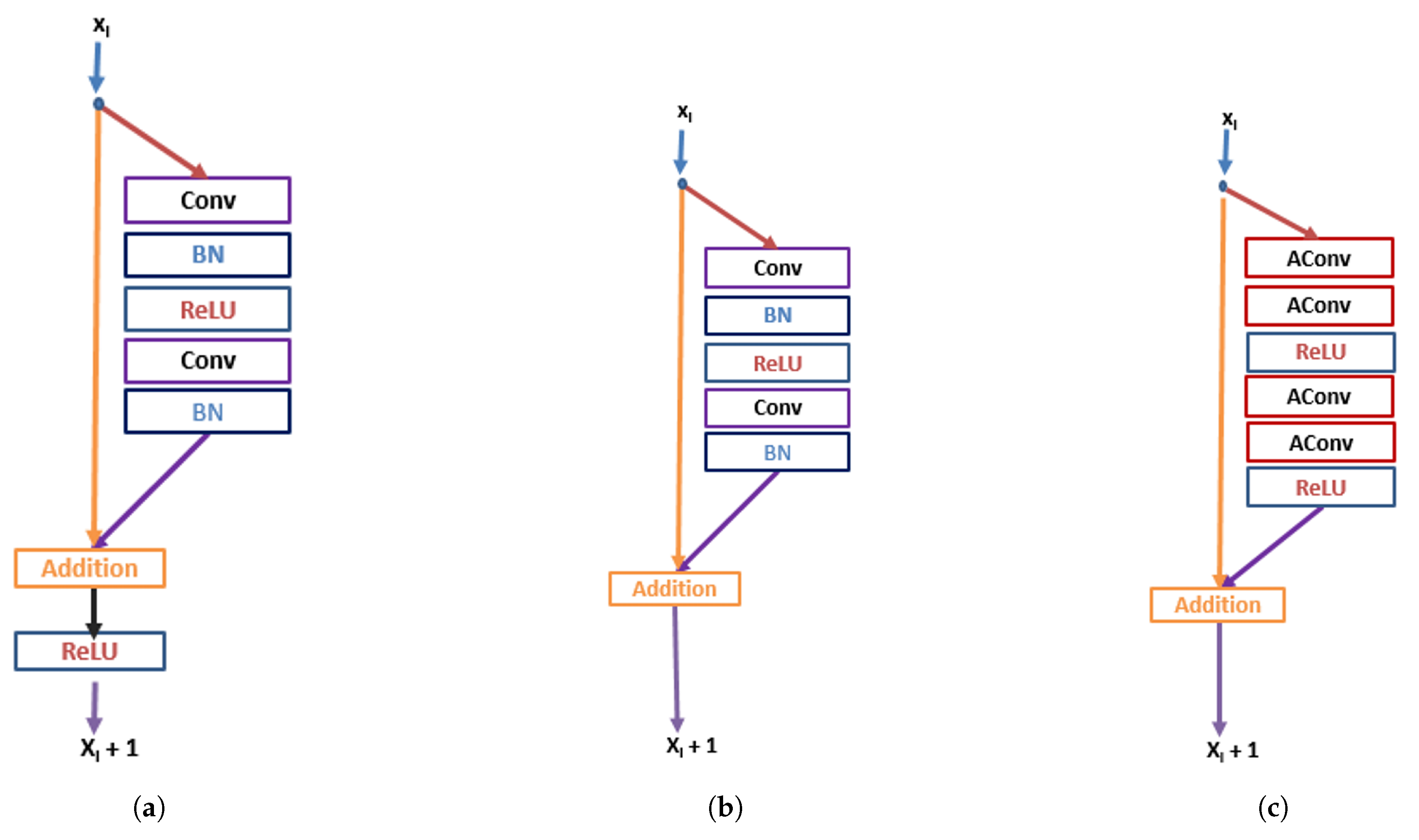
- We proposed a residual asymmetric convolution block to ease the training complexity, as well as reduce the dimensionality of the intermediate layers.
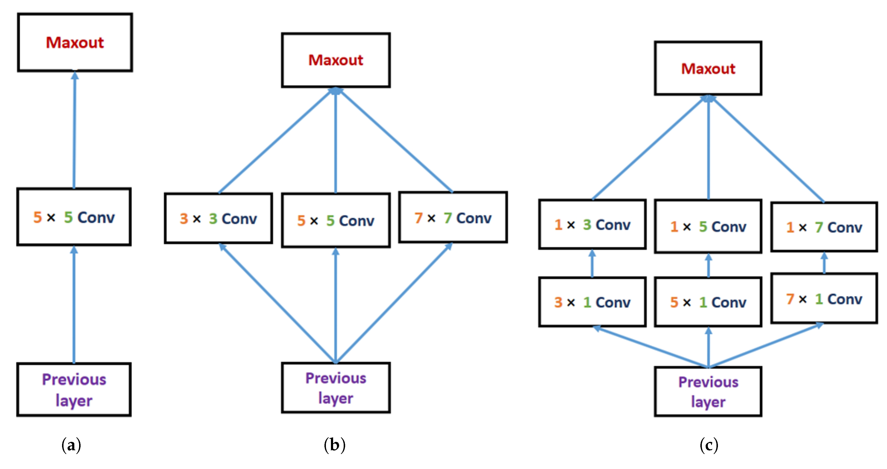
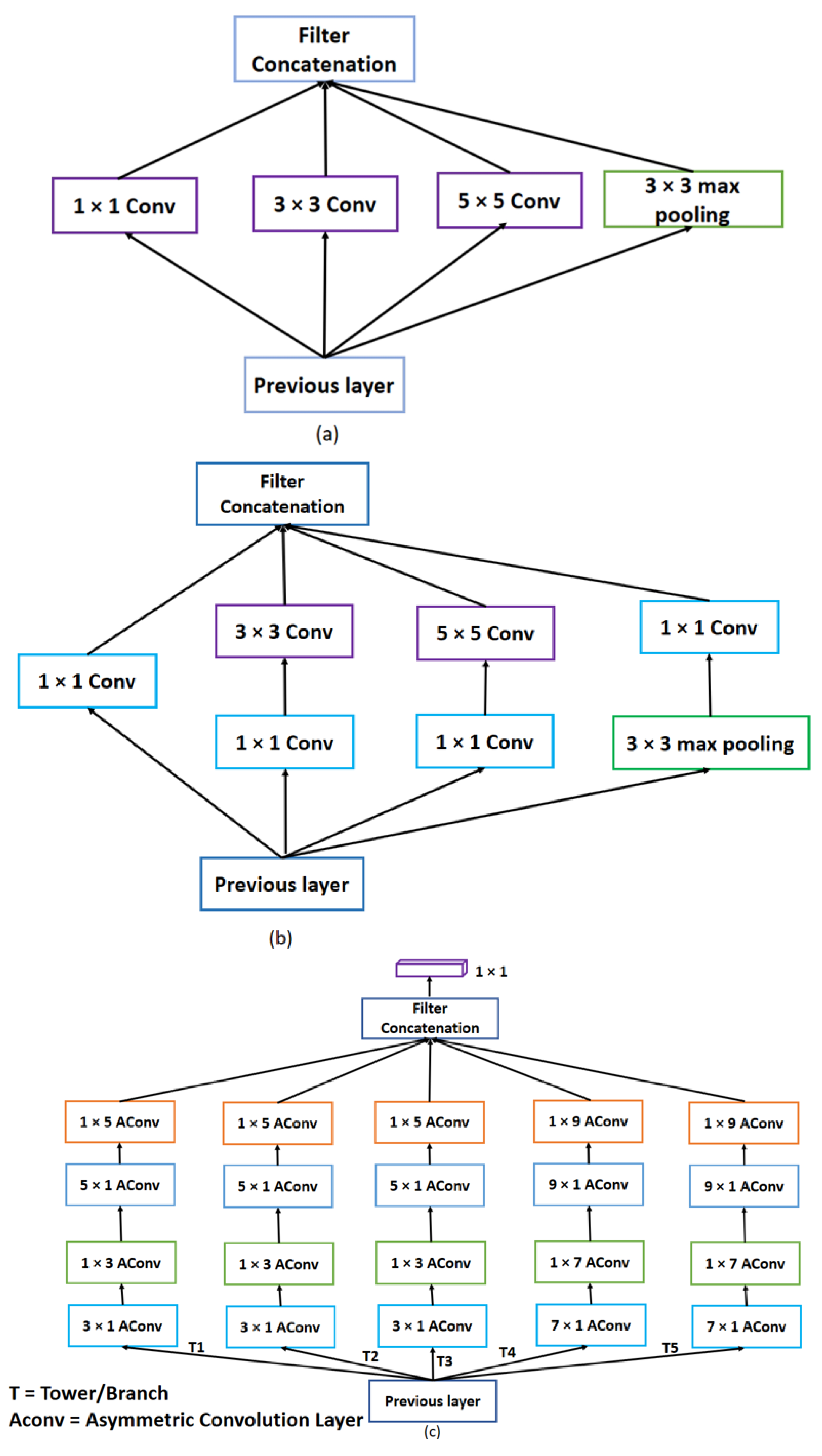
- We also proposed a multi-scale inception block that can extract the multi-scale feature to restore the HR image.
- Based on the inception block, we designed asymmetric convolution deep model that outperforms the traditional convolutional neural networks (CNNs) model on both effectiveness and efficiency.
2. Related Works
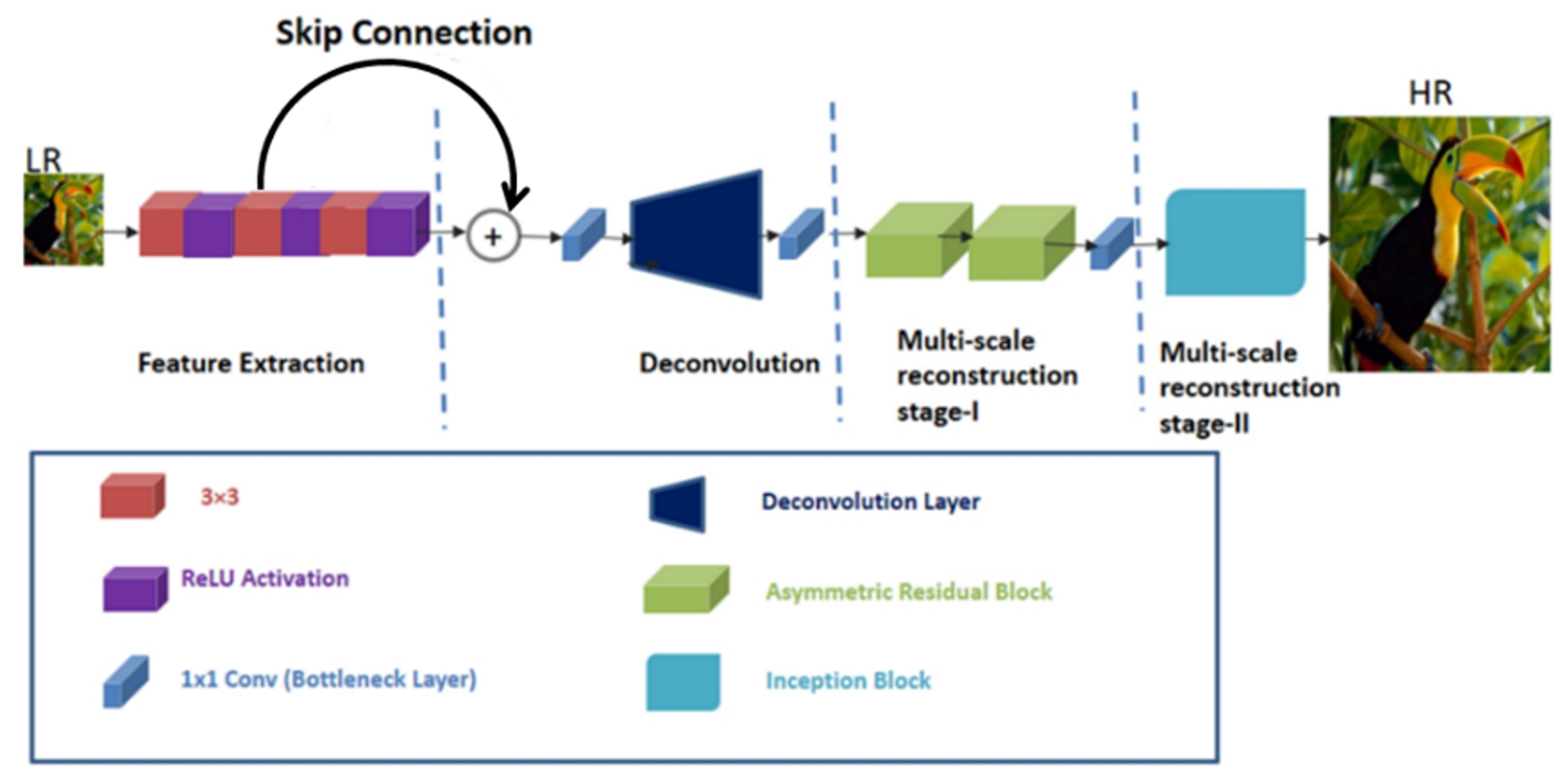
3. Proposed Method
3.1. Feature Extraction
3.2. Deconvolution
3.3. Multi-Scale Reconstruction Stage-I
3.4. Multi-Scale Reconstruction Stage-II
4. Experimental Results
4.1. Training Datasets
4.2. Testing Datasets
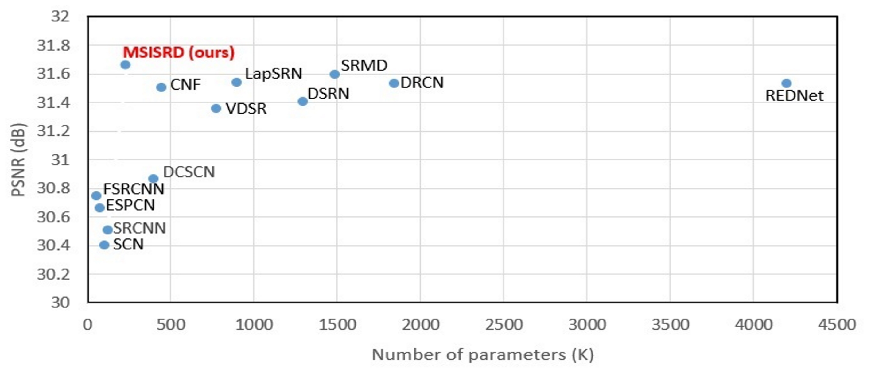
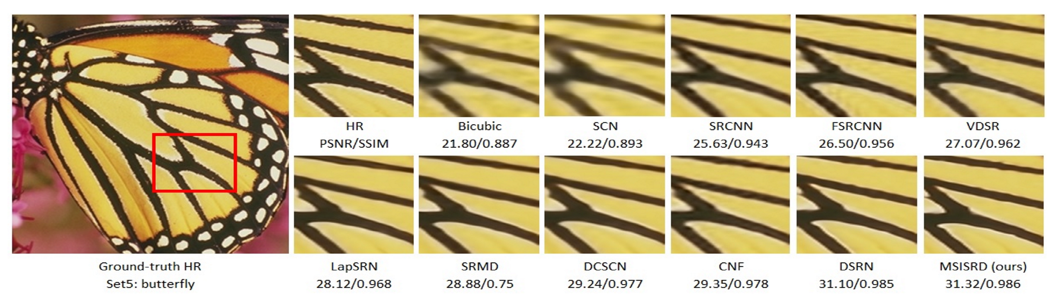
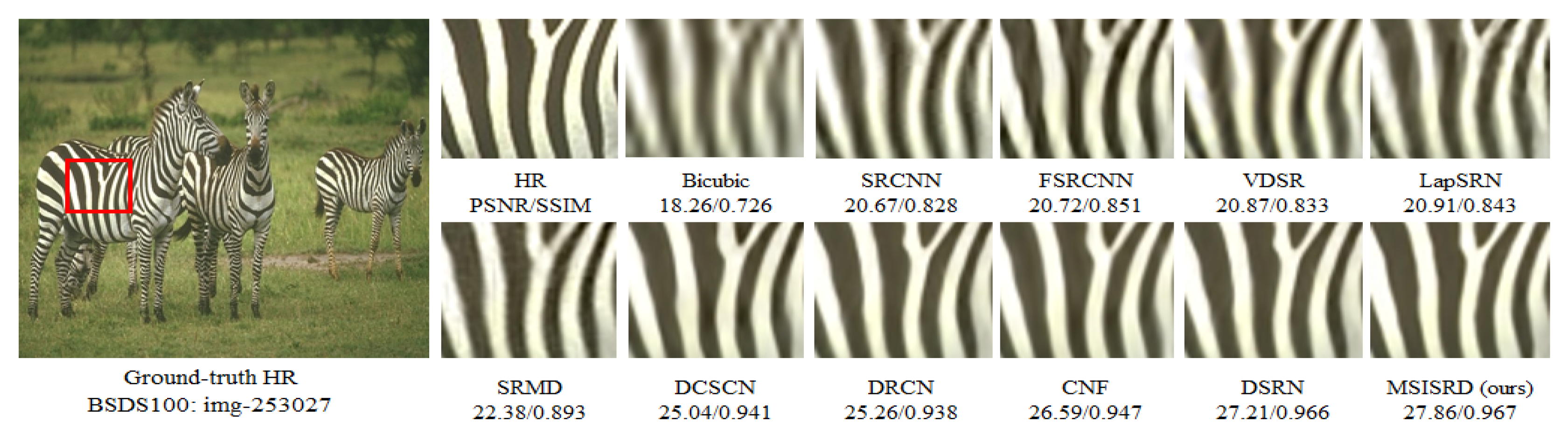
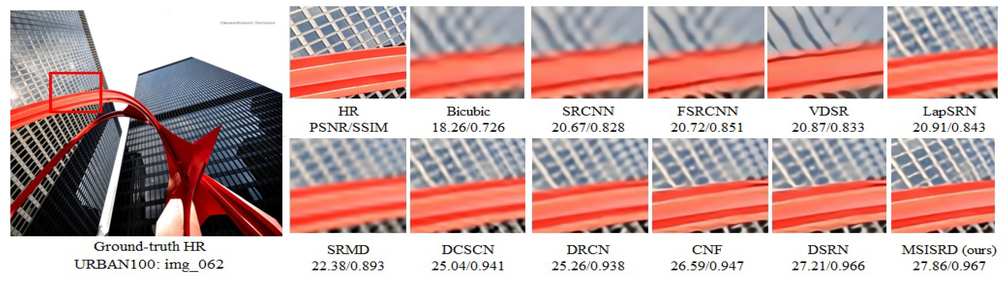
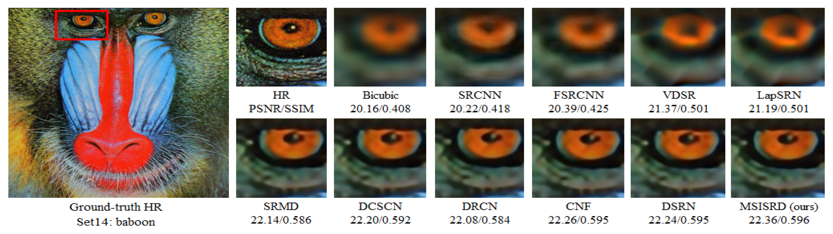
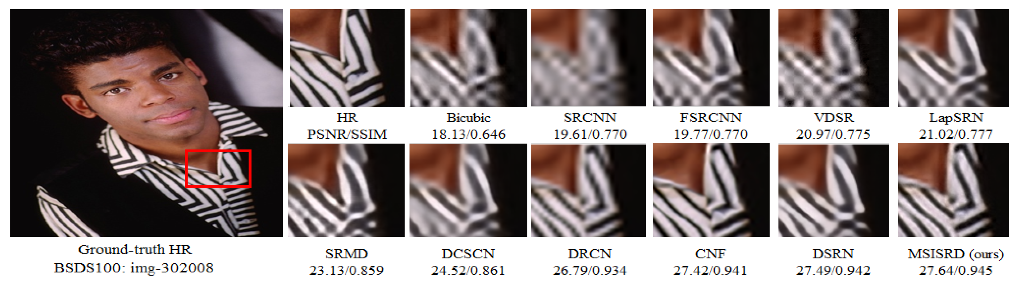
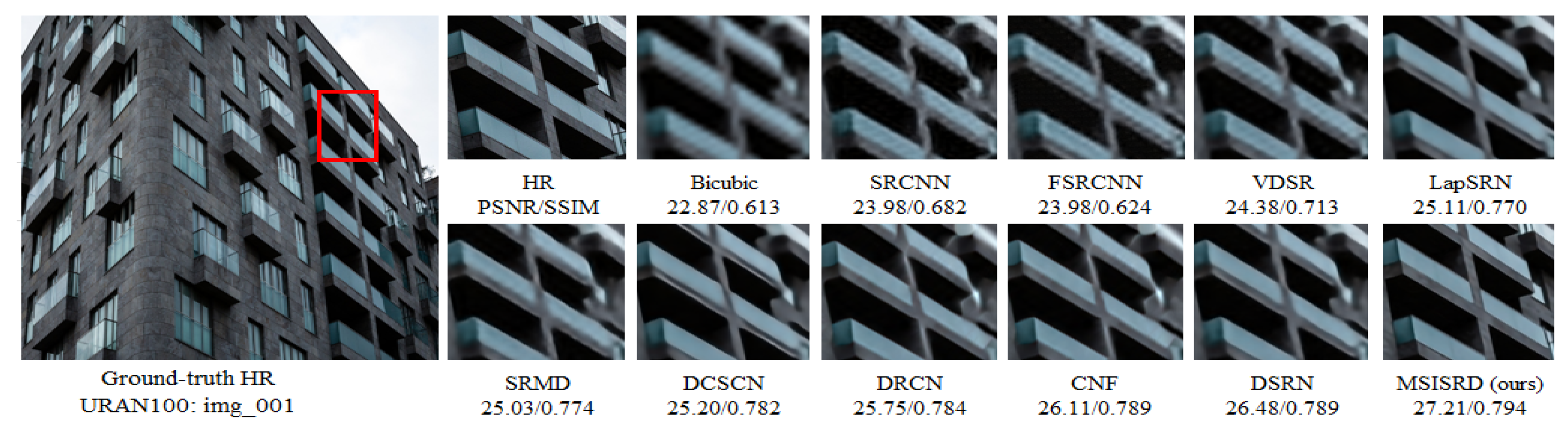
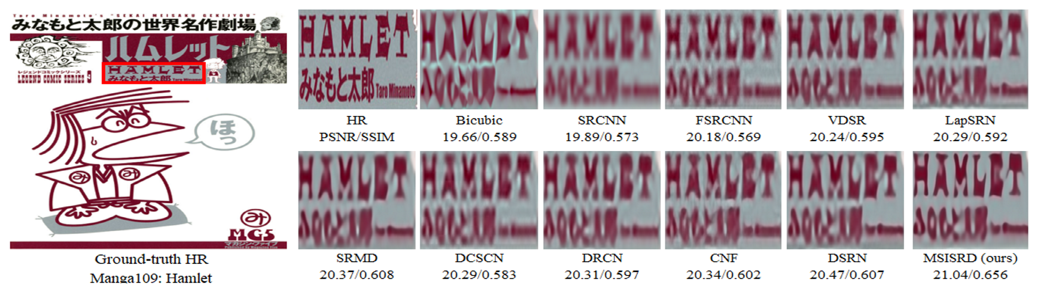
4.3. Comparison with Other Existing State-of-the-Art Methods
5. Conclusions
Author Contributions
Funding
Acknowledgments
Conflicts of Interest
References
- Freeman, W.T.; Jones, T.R.; Pasztor, E.C. Example-based super-resolution. IEEE Comput. Graph. Appl. 2002, 22, 56–65. [Google Scholar] [CrossRef]
- Glasner, D.; Bagon, S.; Irani, M. Super-resolution from a single image. In Proceedings of the 2009 IEEE 12th International Conference on Computer Vision 2009, Kyoto, Japan, 29 September–2 October 2009. [Google Scholar]
- Zhang, L.; Zhang, H.; Shen, H.; Li, P. A super-resolution reconstruction algorithm for surveillance images. Signal Process. 2010, 90, 848–859. [Google Scholar] [CrossRef]
- Gunturk, B.K.; Batur, A.U.; Altunbasak, Y.; Hayes, M.H.; Mersereau, R.M. Eigenface-domain super-resolution for face recognition. IEEE Trans. Image Process. 2003, 12, 597–606. [Google Scholar] [CrossRef] [PubMed]
- Peled, S.; Yeshurun, Y. Superresolution in MRI: Application to human white matter fiber tract visualization by diffusion tensor imaging. Magn. Reson. Med. Off. J. Int. Soc. Magn. Reson. Med. 2001, 45, 29–35. [Google Scholar] [CrossRef]
- Thornton, M.W.; Atkinson, P.M.; Holland, D. Sub-pixel mapping of rural land cover objects from fine spatial resolution satellite sensor imagery using super-resolution pixel-swapping. Int. J. Remote Sens. 2006, 27, 473–491. [Google Scholar] [CrossRef]
- Keys, R. Cubic convolution interpolation for digital image processing. IEEE Trans. Acoust. Speech Signal Process. 1981, 29, 1153–1160. [Google Scholar] [CrossRef]
- Wang, Y.; Wan, W.; Wang, R.; Zhou, X. An improved interpolation algorithm using nearest neighbor from VTK. In Proceedings of the 2010 International Conference on Audio, Language and Image Processing, Shanghai, China, 23–25 November 2010. [Google Scholar]
- Zhang, L.; Wu, X. An edge-guided image interpolation algorithm via directional filtering and data fusion. IEEE Trans. Image Process. 2006, 15, 2226–2238. [Google Scholar] [CrossRef]
- Tai, Y.-W.; Liu, S.; Brown, M.S.; Lin, S. Super resolution using edge prior and single image detail synthesis. In Proceedings of the 2010 IEEE Computer Society Conference on Computer Vision and Pattern Recognition, San Francisco, CA, USA, 13–18 June 2010. [Google Scholar]
- Timofte, R.; De Smet, V.; Van Gool, L. A+: Adjusted anchored neighborhood regression for fast super-resolution. In Proceedings of the Asian Conference on Computer Vision, Singapore, 1–5 November 2014; Springer: Berlin/Heidelberg, Germany, 2014. [Google Scholar]
- Yang, J.; Wright, J.; Huang, T.S.; Ma, Y. Image super-resolution via sparse representation. IEEE Trans. Image Process. 2010, 19, 2861–2873. [Google Scholar] [CrossRef]
- Schulter, S.; Leistner, C.; Bischof, H. Fast and accurate image upscaling with super-resolution forests. In Proceedings of the IEEE Conference on Computer Vision and Pattern Recognition, Boston, MA, USA, 7–12 June 2015. [Google Scholar]
- Du, X.; Qu, X.; He, Y.; Guo, D. Single image super-resolution based on multi-scale competitive convolutional neural network. Sensors 2018, 18, 789. [Google Scholar] [CrossRef]
- Dong, C.; Loy, C.C.; Tang, X. Accelerating the super-resolution convolutional neural network. In Proceedings of the European Conference on Computer Vision, Amsterdam, The Netherlands, 8–16 October 2016; Springer: Berlin/Heidelberg, Germany, 2016. [Google Scholar]
- Kim, J.; Kwon Lee, J.; Mu Lee, K. Accurate image super-resolution using very deep convolutional networks. In Proceedings of the IEEE Conference on Computer Vision and Pattern Recognition, Las Vegas, NV, USA, 26 June–1 July 2016. [Google Scholar]
- Kim, J.; Kwon Lee, J.; Mu Lee, K. Deeply-recursive convolutional network for image super-resolution. In Proceedings of the IEEE Conference on Computer Vision and Pattern Recognition, Las Vegas, NV, USA, 26 June–1 July 2016. [Google Scholar]
- Lai, W.-S.; Huang, J.B.; Ahuja, N.; Yang, M.H. Deep laplacian pyramid networks for fast and accurate superresolution. In Proceedings of the IEEE Conference on Computer Vision and Pattern Recognition, Honolulu, HI, USA, 21–26 July 2017. [Google Scholar]
- Ledig, C.; Theis, L.; Huszar, F.; Caballero, J.; Cunningham, A.; Acosta, A.; Aitken, A.; Tejani, A.; Totz, J.; Wang, Z.; et al. Photo-realistic single image super-resolution using a generative adversarial network. arXiv 2017. [Google Scholar]
- Lim, B.; Son, S.; Kim, H.; Nah, S.; Mu Lee, K. Enhanced deep residual networks for single image super-resolution. In Proceedings of the IEEE Conference on Computer Vision and Pattern Recognition (CVPR) Workshops, Honolulu, HI, USA, 21–26 July 2017. [Google Scholar]
- Tai, Y.; Yang, J.; Liu, X. Image super-resolution via deep recursive residual network. In Proceedings of the IEEE Conference on Computer Vision and Pattern Recognition, Honolulu, HI, USA, 21–26 July 2017. [Google Scholar]
- Timofte, R.; De Smet, V.; Van Gool, L. Anchored neighborhood regression for fast example-based super-resolution. In Proceedings of the IEEE International Conference on Computer Vision, Sydney, Australia, 8–12 April 2013. [Google Scholar]
- Huang, J.-B.; Singh, A.; Ahuja, N. Single image super-resolution from transformed self-exemplars. In Proceedings of the IEEE Conference on Computer Vision and Pattern Recognition, Boston, MA, USA, 7–12 June 2015. [Google Scholar]
- Giachetti, A.; Asuni, N. Real-time artifact-free image upscaling. IEEE Trans. Image Process. 2011, 20, 2760–2768. [Google Scholar] [CrossRef] [PubMed]
- Jianchao, Y.; Wright, J.; Huang, T.; Ma, Y. Image super-resolution as sparse representation of raw image patches. In Proceedings of the IEEE Conference on Computer Vision and Pattern Recognition, Anchorage, AK, USA, 24–26 June 2008. [Google Scholar]
- Dong, C.; Loy, C.C.; He, K.; Tang, X. Learning a deep convolutional network for image super-resolution. In Proceedings of the European Conference on Computer Vision, Zurich, Switzerland, 6–12 September 2014; Springer: Berlin/Heidelberg, Germany, 2014. [Google Scholar]
- Wang, Z.; Liu, D.; Yang, J.; Han, W.; Huang, T. Deep networks for image super-resolution with sparse prior. In Proceedings of the IEEE International Conference on Computer Vision, Santiago, Chile, 7–13 December 2015. [Google Scholar]
- Shi, W.; Caballero, J.; Huszár, F.; Totz, J.; Aitken, A.P.; Bishop, R.; Rueckert, D.; Wang, Z.; Magic Pony Technology; Imperial College London. Real-time single image and video super-resolution using an efficient sub-pixel convolutional neural network. In Proceedings of the IEEE Conference on Computer Vision and Pattern Recognition, Las Vegas, NV, USA, 26 June–1 July 2016. [Google Scholar]
- Ronneberger, O.; Fischer, P.; Brox, T. U-net: Convolutional networks for biomedical image segmentation. In Proceedings of the International Conference on Medical Image Computing and Computer-Assisted Intervention, Munich, Germany, 5–9 October 2015; Springer: Berlin/Heidelberg, Germany, 2015. [Google Scholar]
- Mao, X.; Shen, C.; Yang, Y.-B. Image restoration using very deep convolutional encoder-decoder networks with symmetric skip connections. In Proceedings of the Advances in Neural Information Processing Systems, Barcelona, Spain, 5–10 December 2016. [Google Scholar]
- Wang, Y.; Wang, L.; Wang, H.; Li, P. End-to-End Image Super-Resolution via Deep and Shallow Convolutional Networks; IEEE: Piscataway, NJ, USA, 2019; Volume 7, pp. 31959–31970. [Google Scholar]
- Zeiler, M.D.; Taylor, G.W.; Fergus, R. Adaptive deconvolutional networks for mid and high level feature learning. In Proceedings of the 2011 IEEE International Conference on Computer Vision (ICCV), Barcelona, Spain, 6–13 November 2011. [Google Scholar]
- Hui, Z.; Wang, X.; Gao, X. Fast and Accurate Single Image Super-Resolution via Information Distillation Network. In Proceedings of the IEEE Conference on Computer Vision and Pattern Recognition, Salt Lake City, UT, USA, 18–22 June 2018. [Google Scholar]
- He, K.; Zhang, X.; Ren, S.; Sun, J. Deep residual learning for image recognition. In Proceedings of the IEEE Conference on Computer Vision and Pattern Recognition, Las Vegas, NV, USA, 26 June–1 July 2016. [Google Scholar]
- Ioffe, S.; Szegedy, C. Batch normalization: Accelerating deep network training by reducing internal covariate shift. arXiv 2015, arXiv:1502.03167. [Google Scholar]
- Ren, H.; El-Khamy, M.; Lee, J. Image super resolution based on fusing multiple convolution neural networks. In Proceedings of the IEEE Conference on Computer Vision and Pattern Recognition, Honolulu, HI, USA, 21–26 July 2017. [Google Scholar]
- Yamanaka, J.; Kuwashima, S.; Kurita, T. Fast and accurate image super resolution by deep CNN with skip connection and network in network. In Neural Information Processing; Springer: Cham, Switzerland, 2017. [Google Scholar]
- Han, W.; Chang, S.; Liu, D.; Yu, M.; Witbrock, M.; Huang, T.S. Image super-resolution via dual-state recurrent networks. In Proceedings of the IEEE Conference on Computer Vision and Pattern Recognition, Salt Lake City, UT, USA, 18–22 June 2018. [Google Scholar]
- Zhang, K.; Zuo, W.; Zhang, L. Learning a single convolutional super-resolution network for multiple degradations. In Proceedings of the IEEE Conference on Computer Vision and Pattern Recognition, Salt Lake City, UT, USA, 18–22 June 2018. [Google Scholar]
- Zhang, K.; Zuo, W.; Gu, S.; Zhang, L. Learning deep CNN denoiser prior for image restoration. In Proceedings of the IEEE Conference on Computer Vision and Pattern Recognition, Honolulu, HI, USA, 21–26 July 2017. [Google Scholar]
- Mei, K.; Jiang, A.; Li, J.; Ye, J.; Wang, M. An Effective Single-Image Super-Resolution Model Using Squeeze-and-Excitation Networks. In Proceedings of the International Conference on Neural Information Processing, Siem Reap, Cambodia, 13–16 December 2018; Springer: Cham, Switzerland, 2018; pp. 542–553. [Google Scholar]
- Nair, V.; Hinton, G.E. Rectified linear units improve restricted boltzmann machines. In Proceedings of the 27th International Conference on Machine Learning (ICML-10), Haifa, Israel, 21–24 June 2010. [Google Scholar]
- Chu, X.; Zhang, B.; Xu, R.; Ma, H. Multi-objective reinforced evolution in mobile neural architecture search. arXiv 2019, arXiv:1901.01074. [Google Scholar]
- Haris, M.; Shakhnarovich, G.; Ukita, N. Deep backprojection networks for super-resolution. In Proceedings of the IEEE Conference on Computer Vision and Pattern Recognition, Salt Lake City, UT, USA, 18–22 June 2018. [Google Scholar]
- Simonyan, K.; Zisserman, A. Very deep convolutional networks for large-scale image recognition. arXiv 2014, arXiv:1409.1556. [Google Scholar]
- Zhang, K.; Zuo, W.; Chen, Y.; Meng, D.; Zhang, L. Beyond a gaussian denoiser: Residual learning of deep cnn for image denoising. IEEE Trans. Image Process. 2017, 26, 3142–3155. [Google Scholar] [CrossRef] [PubMed]
- Romera, E.; Alvarez, J.M.; Bergasa, L.M.; Arroyo, R. Efficient convnet for real-time semantic segmentation. In Proceedings of the 2017 IEEE Intelligent Vehicles Symposium (IV), Los Angeles, CA, USA, 11–14 June 2017. [Google Scholar]
- Szegedy, C.; Vanhoucke, V.; Ioffe, S.; Shlens, J.; Wojna, Z. Rethinking the inception architecture for computer vision. In Proceedings of the IEEE Conference on Computer Vision and Pattern Recognition, Las Vegas, NV, USA, 26 June–1 July 2016. [Google Scholar]
- Mahapatra, D.; Bozorgtabar, B.; Hewavitharanage, S.; Garnavi, R. Image super resolution using generative adversarial networks and local saliency maps for retinal image analysis. In Proceedings of the International Conference on Medical Image Computing and Computer-Assisted Intervention, Quebec City, QC, Canada, 10–14 September 2017; Springer: Cham, Switzerland; pp. 382–390. [Google Scholar]
- Lin, M.; Chen, Q.; Yan, S. Network in network. arXiv 2013, arXiv:1312.4400. [Google Scholar]
- Szegedy, C.; Liu, W.; Jia, Y.; Sermanet, P.; Reed, S.; Anguelov, D.; Erhan, D.; Vanhoucke, V.; Rabinovich, A. Going deeper with convolutions. In Proceedings of the IEEE Conference on Computer Vision and Pattern Recognition, Boston, MA, USA, 7–12 June 2015. [Google Scholar]
- Szegedy, C.; Ioffe, S.; Vanhoucke, V.; Alemi, A.A. Inception-v4, inception-resnet and the impact of residual connections on learning. In Proceedings of the Thirty-First AAAI Conference on Artificial Intelligence, San Francisco, CA, USA, 4–9 February 2017. [Google Scholar]
- Khened, M.; Kollerathu, V.A.; Krishnamurthi, G. Fully convolutional multi-scale residual DenseNets for cardiac segmentation and automated cardiac diagnosis using ensemble of classifiers. Med. Image Anal. 2019, 51, 21–45. [Google Scholar] [CrossRef]
- Zhang, H.; Hong, X. Recent progresses on object detection: A brief review. Multimed. Tools Appl. 2019, 78, 1–39. [Google Scholar] [CrossRef]
- Krig, S. Feature learning and deep learning architecture survey. In Computer Vision Metrics; Springer: Cham, Switzerland, 2016; pp. 375–514. [Google Scholar]
- Wang, Z.; Bovik, A.C.; Sheikh, H.R.; Simoncelli, E.P. Image quality assessment: From error visibility to structural similarity. IEEE Trans. Image Process. 2004, 13, 600–612. [Google Scholar] [CrossRef]
- Yang, C.-Y.; Ma, C.; Yang, M.-H. Single-image super-resolution: A benchmark. In Proceedings of the European Conference on Computer Vision, Zurich, Switzerland, 6–12 September 2014; Springer: Berlin/Heidelberg, Germany, 2014. [Google Scholar]
- Martin, D.; Fowlkes, C.; Tal, D.; Malik, J. A database of human segmented natural images and its application to evaluating segmentation algorithms and measuring ecological statistics. In Proceedings of the Eighth International Conference On Computer Vision (ICCV-01), Vancouver, BC, Canada, 7–14 July 2001. [Google Scholar]
- Available online: https://github.com/MarkPrecursor/ (accessed on 26 November 2018).
- Chollet, F. Keras: The Python Deep Learning Library. Available online: https://keras.io/ (accessed on 6 August 2019).
- Kingma, D.P.; Ba, J. Adam: A method for stochastic optimization. arXiv 2014, arXiv:1412.6980. [Google Scholar]
- Bevilacqua, M.; Roumy, A.; Guillemot, C.; Alberi-Morel, M.L. Low-complexity single-image super-resolution based on nonnegative neighbor embedding. In Proceedings of the British Machine Vision Conference, Surrey, UK, 3–7 September 2012. [Google Scholar]
- Zeyde, R.; Elad, M.; Protter, M. On Single Image Scale-Up Using Sparse-Representations. In Proceedings of the International Conference on Curves and Surfaces, Oslo, Norway, 28 June–3 July 2012; pp. 711–730. [Google Scholar]
- Matsui, Y.; Ito, K.; Aramaki, Y.; Fujimoto, A.; Ogawa, T.; Yamasaki, T.; Aizawa, K. Sketch-based manga retrieval using manga109 dataset. Multimed. Tools Appl. 2017, 76, 21811–21838. [Google Scholar] [CrossRef]
- Zhang, Y.; Li, K.; Li, K.; Wang, L.; Zhong, B.; Fu, Y. Image super-resolution using very deep residual channel attention networks. In Proceedings of the European Conference on Computer Vision (ECCV), Munich, Germany, 8–14 September 2018; pp. 286–301. [Google Scholar]
- Zhu, L.; Zhan, S.; Zhang, H. Stacked U-shape networks with channel-wise attention for image super-resolution. Neurocomputing 2019, 345, 58–66. [Google Scholar] [CrossRef]
- Shamsolmoali, P.; Zhang, J.; Yang, J. Image super resolution by dilated dense progressive network. Image Vision Comput. 2019, 88, 9–18. [Google Scholar] [CrossRef]
- Shen, M.; Yu, P.; Wang, R.; Yang, J.; Xue, L.; Hu, M. Multipath feedforward network for single image super-resolution. Multimed. Tools Appl. 2019, 78, 1–20. [Google Scholar] [CrossRef]
- Li, J.; Zhou, Y. Image Super-Resolution Based on Dense Convolutional Network. In Proceedings of the Chinese Conference on Pattern Recognition and Computer Vision (PRCV), Guangzhou, China, 23–26 November 2018; Springer: Cham, Switzerland; pp. 134–145. [Google Scholar]
- Kim, H.; Choi, M.; Lim, B.; Mu Lee, K. Task-Aware Image Downscaling. In Proceedings of the European Conference on Computer Vision (ECCV), Munich, Germany, 8–14 September 2018. [Google Scholar]
- Wang, X.; Yu, K.; Wu, S.; Gu, J.; Liu, Y.; Dong, C.; Qiao, Y.; Loy, C.C. Esrgan: Enhanced super-resolution generative adversarial networks. In Proceedings of the European Conference on Computer Vision (ECCV), Munich, Germany, 8–14 September 2018. [Google Scholar]
- Luo, X.; Chen, R.; Xie, Y.; Qu, Y.; Li, C. Bi-GANs-ST for perceptual image super-resolution. In Proceedings of the European Conference on Computer Vision (ECCV), Munich, Germany, 8–14 September 2018. [Google Scholar]


| Kernel Size | No: of Layers | No: of Filters | Image Patch Size | No: of Parameters |
|---|---|---|---|---|
| 1 | 10 | 900 | ||
| and | 2 | 10 | 600 | |
| 1 | 10 | 2500 | ||
| and | 2 | 10 | 1000 | |
| 1 | 10 | 4900 | ||
| and | 2 | 10 | 1400 | |
| 1 | 10 | 8100 | ||
| and | 2 | 10 | 1800 | |
| 1 | 10 | 12,100 | ||
| and | 2 | 10 | 2200 |
| Method | Factor | Params | Set5 [62] | Set14 [63] | BSDS100 [58] | Urban100 [23] | Manga109 [64] |
|---|---|---|---|---|---|---|---|
| PSNR/SSIM | PSNR/SSIM | PSNR/SSIM | PSNR/SSIM | PSNR/SSIM | |||
| Bicubic | - | 33.69/0.931 | 30.25/0.870 | 29.57/0.844 | 26.89/0.841 | 30.86/0.936 | |
| A+ [11] | - | 36.60/0.955 | 32.32/0.906 | 31.24/0.887 | 29.25/0.895 | 35.37/0.968 | |
| RFL [13] | - | 36.59/0.954 | 32.29/0.905 | 31.18/0.885 | 29.14/0.891 | 35.12/0.966 | |
| SelfExSR [23] | - | 36.60/0.955 | 32.24/0.904 | 31.20/0.887 | 29.55/0.898 | 35.82/0.969 | |
| SRCNN [26] | 57k | 36.72/0.955 | 32.51/0.908 | 31.38/0.889 | 29.53/0.896 | 35.76/0.968 | |
| ESPCN [28] | 20k | 37.00/0.955 | 32.75/0.909 | 31.51/0.893 | 29.87/0.906 | 36.21/0.969 | |
| FSRCNN [15] | 12k | 37.05/0.956 | 32.66/0.909 | 31.53/0.892 | 29.88/0.902 | 36.67/0.971 | |
| SCN [27] | 42k | 36.58/0.954 | 32.35/0.905 | 31.26/0.885 | 29.52/0.897 | 35.51/0.967 | |
| VDSR [16] | 665k | 37.53/0.959 | 33.05/0.913 | 31.90/0.896 | 30.77/0.914 | 37.22/0.975 | |
| DCSCN [37] | 244k | 37.62/0.959 | 33.05/0.912 | 31.91/0.895 | 30.77/0.910 | 37.25/0.974 | |
| LapSRN [18] | 813k | 37.52/0.959 | 33.08/0.913 | 31.80/0.895 | 30.41/0.910 | 37.27/0.974 | |
| DRCN [17] | 1774k | 37.63/0.959 | 33.06/0.912 | 31.85/0.895 | 30.76/0.914 | 37.63/0.974 | |
| SrSENet [41] | - | 37.56/0.958 | 33.14/0.911 | 31.84/0.896 | 30.73/0.917 | 37.43/0.974 | |
| MOREMNAS-D [43] | 664k | 37.57/0.958 | 33.25/0.914 | 31.94/0.896 | 31.25/0.919 | 37.65/0.975 | |
| SRMD [39] | 1482 | 37.53/0.959 | 33.12/0.914 | 31.90/0.896 | 30.89/0.916 | 37.24/0.974 | |
| REDNet [30] | 4131k | 37.66/0.959 | 32.94/0.914 | 31.99/0.897 | 30.91/0.915 | 37.45/0.974 | |
| DSRN [38] | 1200k | 37.66/0.959 | 33.15/0.913 | 32.10/0.897 | 30.97/0.916 | 37.49/0.973 | |
| CNF [36] | 337k | 37.66/0.959 | 33.38/0.914 | 31.91/0.896 | 31.15/0.914 | 37.64/0.974 | |
| MSISRD (ours) | 240k | 37.80/0.960 | 33.84/0.920 | 32.09/0.895 | 31.10/0.913 | 37.70/0.975 | |
| Bicubic | - | 28.43/0.811 | 26.01/0.704 | 25.97/0.670 | 23.15/0.660 | 24.93/0.790 | |
| A+ [11] | - | 30.32/0.860 | 27.34/0.751 | 26.83/0.711 | 24.34/0.721 | 27.03/0.851 | |
| RFL [13] | - | 30.17/0.855 | 27.24/0.747 | 26.76/0.708 | 24.20/0.712 | 26.80/0.841 | |
| SelfExSR [23] | - | 30.34/0.862 | 27.41/0.753 | 26.84/0.713 | 24.83/0.740 | 27.83/0.8663 | |
| SRCNN [26] | 57k | 30.49/0.863 | 27.52/0.753 | 26.91/0.712 | 24.53/0.725 | 27.66/0.859 | |
| ESPCN [28] | 20k | 30.66/0.864 | 27.71/0.756 | 26.98/0.712 | 24.60/0.736 | 27.70/0.856 | |
| FSRCNN [15] | 12k | 30.72/0.866 | 27.61/0.755 | 26.98/0.715 | 24.62/0.728 | 27.90/0.861 | |
| SCN [27] | 42k | 30.41/0.863 | 27.39/0.751 | 26.88/0.711 | 24.52/0.726 | 27.39/0.857 | |
| VDSR [16] | 665k | 31.35/0.883 | 28.02/0.768 | 27.29/0.726 | 25.18/0.754 | 28.83/0.887 | |
| DCSCN [37] | 244k | 30.86/0.871 | 27.74/0.770 | 27.04/0.725 | 25.20/0.754 | 28.99/0.888 | |
| LapSRN [18] | 813k | 31.54/0.885 | 28.19/0.772 | 27.32/0.727 | 25.21/0.756 | 29.09/0.890 | |
| DRCN [17] | 1774k | 31.54/0.884 | 28.03/0.768 | 27.24/0.725 | 25.14/0.752 | 28.98/0.887 | |
| SrSENet [41] | - | 31.40/0.881 | 28.10/0.766 | 27.29/0.720 | 25.21/0.762 | 29.08/0.888 | |
| SRMD [39] | 1482 | 31.59/0.887 | 28.15/0.772 | 27.34 /0.728 | 25.34/0.761 | 30.49/0.890 | |
| REDNet [30] | 4131k | 31.51/0.886 | 27.86/0.771 | 27.40/0.728 | 25.35/0.758 | 28.96/0.887 | |
| DSRN [38] | 1200 | 31.40/0.883 | 28.07/0.770 | 27.25/0.724 | 25.08/0.747 | 30.15/0.890 | |
| CNF [36] | 337k | 31.55/0.885 | 28.15/0.768 | 27.32/0.725 | 25.32/0.753 | 30.47/0.890 | |
| MSISRD (ours) | 240k | 31.62/0.886 | 28.51/0.771 | 27.33/0.727 | 25.42/0.757 | 31.61/0.891 | |
| Bicubic | - | 24.40/0.658 | 23.10/0.566 | 23.67/0.548 | 20.74/0.516 | 21.47/0.650 | |
| A+ [11] | - | 25.53/0.693 | 23.89/0.595 | 24.21/0.569 | 21.37/0.546 | 22.39/0.681 | |
| RFL [13] | - | 25.38/0.679 | 23.79/0.587 | 24.13/0.563 | 21.27/0.536 | 22.28/0.669 | |
| SelfExSR [23] | - | 25.49/0.703 | 23.92/0.601 | 24.19/0.568 | 21.81/0.577 | 22.99/0.719 | |
| SRCNN [26] | 57k | 25.33/0.690 | 23.76/0.591 | 24.13/0.566 | 21.29/0.544 | 22.46/0.695 | |
| ESPCN [28] | 20k | 25.75/0.673 | 24.21/0.510 | 24.73/0.527 | 21.59/0.542 | 22.83/0.671 | |
| FSRCNN [15] | 12k | 25.60/0.697 | 24.00/0.599 | 24.31/0.572 | 21.45/0.550 | 22.72/0.692 | |
| SCN [27] | 42k | 25.59/0.706 | 24.02/0.603 | 24.30/0.573 | 21.52/0.560 | 22.68/0.701 | |
| VDSR [16] | 665k | 25.93/0.724 | 24.26/0.614 | 24.49/0.583 | 21.70/0.571 | 23.16/0.725 | |
| DCSCN [37] | 244k | 24.96/0.673 | 23.50/0.576 | 24.00/0.554 | 21.75/0.571 | 23.33/0.731 | |
| LapSRN [18] | 813k | 26.15/0.738 | 24.35/0.620 | 24.54/0.586 | 21.81/0.581 | 23.39/0.735 | |
| DRCN [17] | 1775k | 25.93/0.723 | 24.25/0.614 | 24.49/0.582 | 21.71/0.571 | 23.20/0.724 | |
| SrSENet [41] | - | 26.10/0.703 | 24.38/0.586 | 24.59/0.539 | 21.88/0.571 | 23.54/0.722 | |
| MSISRD (ours) | 240k | 26.26/0.737 | 24.38/0.621 | 24.73/0.586 | 22.53/0.582 | 23.50/0.738 |
| Models | PSNR/SSIM [56] | Parameters |
|---|---|---|
| SRCNN [26] | 30.50/0.863 | 57k |
| ESPCN [28] | 30.66/0.864 | 20k |
| FSRCNN [15] | 30.72/0.866 | 12k |
| SCN [27] | 30.41/0.863 | 42k |
| VDSR [16] | 31.35/0.883 | 665k |
| DCSCN [37] | 30.86/0.871 | 244k |
| LapSRN [50] | 31.54/0.885 | 813k |
| DRCN [17] | 31.54/0.884 | 1775k |
| SRMD [39] | 31.59/0.887 | 1482k |
| REDNet [30] | 31.51/0.886 | 4131k |
| DSRN [38] | 31.40/0.883 | 1200k |
| CNF [36] | 31.55/0.885 | 337k |
| MSISRD (ours) | 31.62/0.886 | 240k |
© 2019 by the authors. Licensee MDPI, Basel, Switzerland. This article is an open access article distributed under the terms and conditions of the Creative Commons Attribution (CC BY) license (http://creativecommons.org/licenses/by/4.0/).
Share and Cite
Muhammad, W.; Aramvith, S. Multi-Scale Inception Based Super-Resolution Using Deep Learning Approach. Electronics 2019, 8, 892. https://doi.org/10.3390/electronics8080892
Muhammad W, Aramvith S. Multi-Scale Inception Based Super-Resolution Using Deep Learning Approach. Electronics. 2019; 8(8):892. https://doi.org/10.3390/electronics8080892
Chicago/Turabian StyleMuhammad, Wazir, and Supavadee Aramvith. 2019. "Multi-Scale Inception Based Super-Resolution Using Deep Learning Approach" Electronics 8, no. 8: 892. https://doi.org/10.3390/electronics8080892
APA StyleMuhammad, W., & Aramvith, S. (2019). Multi-Scale Inception Based Super-Resolution Using Deep Learning Approach. Electronics, 8(8), 892. https://doi.org/10.3390/electronics8080892