Control Design of LCL Type Grid-Connected Inverter Based on State Feedback Linearization

1
Jiangsu Province Laboratory of Mining Electric and Automation, China University of Mining and Technology, Xuzhou 221116, China
2
School of Electrical and Power Engineering, China University of Mining and Technology, Xuzhou 221116, China
*
Author to whom correspondence should be addressed.
Electronics 2019, 8(8), 877; https://doi.org/10.3390/electronics8080877
Submission received: 11 July 2019
/
Revised: 2 August 2019
/
Accepted: 3 August 2019
/
Published: 7 August 2019
(This article belongs to the Special Issue Power Converters in Power Electronics)
Abstract
:Control strategy is the key technology of power electronic converter equipment. In order to solve the problem of controller design, a general design method is presented in this paper, which is more convenient to use computer machine learning and provides design rules for high-order power electronic system. With the higher order system Lie derivative, the nonlinear system is mapped to a controllable standard type, and then classical linear system control method is adopted to design the controller. The simulation and experimental results show that the two controllers have good steady-state control performance and dynamic response performance.
1. Introduction
As the main equipment of an AC power system, grid-connected voltage source inverters (VSI) have been widely used in recent years, such as photovoltaic inverters [1], Pulse Width Modulation Pulse Width Modulation (PWM) rectifiers [2], static var generators [3], active power filters [4], etc.
The filter is an important part of the inverter, the structure of which directly determines the mathematical model and control mode of the inverter. Nowadays, a Inductance-Capacitance-Inductance (LCL) filter, with the advantages of small size, low cost and high harmonic attenuation for high frequency current, is widely used in voltage source type grid-connected converters. Considering that the LCL filter is the 3-order system, the damping of the system is small, resulting in a resonant peak of the grid-side inductance current. This phenomenon will adversely affect the safe and stable operation of grid-connected system. In order to improve the damping characteristics of the system, additional system damping is required. Active damping control method is commonly used at present stage [5]. With the state variables feedback, the traditional proportional integral controller can be used to achieve the grid-side inductance current control.
However, for nonlinear power electronic devices, this design method of the controller is based on small signal modeling [6] and harmonic linearization. As the coupling and high order terms in the system are ignored in the Taylor series calculation, the obtained controller is suitable for working at steady working point with poor performance in other control domains [7].
In order to solve the global control problem, many solutions have been put forward [8,9]. Among them, the state feedback linearization method that develops from differential geometry [10,11] has become an effective way to solve the nonlinear power electronics system control problems. Based on the differential homeomorphism, Lie derivative is used to analyze the numerical relation between the state variables, the input variables, and the output variables. Then, the necessary and sufficient conditions for controllability and observability of nonlinear control systems can be established. Choi et al. proposed a feedback linearization direct torque control for the permanent magnet synchronous motor [12]. In addition, the drive flux and torque ripple were suppressed. Yang et al. combined feedback linearization and sliding mode variable structure control to complete the control of three-phase four-leg inverter [13]. This method was used to decouple the torque and stator flux of the inductive motor by Lascu et al. [14]. Yang et al. applied the state feedback control to the Modular Multilevel Converter (MMC) system and analyzed the performance characteristics of the system [15].
Different from the local approximate linearization method, the feedback decoupling is achieved by adopting this nonlinear algorithm without ignoring the higher-order terms. However, the commonly used feedback linearization algorithm at the present stage is mostly used in the 2-order or 1-order system. The research on the controller design of high-order or other complex systems is rare. In addition, when the order of the controlled object is high, whether the state feedback control can be transformed into a simple form has not been analyzed by literatures.
In order to achieve the control of high-order power electronic systems, the design of controller based on LCL filter type grid-connected inverters is studied in this paper. For the 3-order control system, two controller design methods based on state feedback linearization are proposed in this paper. Lie derivative vector field is used to solve the system relationship and design the decoupling matrix. Through the nonlinear mapping, the nonlinear system can be mapped to a controllable standard form. Then, the classical linear system control method, which can be designed easily, is applicable for the controller design. Finally, the performance of the two controllers is compared and analyzed by simulations and experiments.
2. Single Closed-Loop Controller Design Based on State Feedback Linearization
2.1. Model of the Three-Phase Three-Leg Grid-Connected Inverter
Figure 1 shows the structure of the three-phase three-leg LCL grid-connected inverter. L1 and L2 denote the inverter side inductance and the grid-side inductance, respectively.
As the model has been analyzed by many literatures, this paper does not repeat the description. The mathematical model of inverter in dq coordinate axis is given directly as
where the state variables represent the inverter side inductance current, the filter capacitor voltage, the grid-side inductance current and the DC voltage in the synchronous reference coordinate system, respectively. ed and eq represent grid voltage in the synchronous reference coordinate system, respectively. md and mq represent the nonlinear pulse width modulation variables, respectively. ω represents the fundamental angular frequency of the system.
According to (1), due to the mutual inductance and mutual capacitance, the inductance current and the capacitance voltage is coupled in the synchronous reference coordinate system.
Usually, the voltage source grid-connected inverter system is a double closed loop structure. The outer loop controls DC voltage, and the inner loop controls AC current. However, for the different structure like the PV system, the DC voltage may not need to be controlled. Considering the generality, only the current inner loop is analyzed. Due to the LCL filter, the system can be regarded as a 2-input 2-output system. At the same time, the existence of LCL filter capacitor, which introduces a pair of conjugate pure imaginary roots to cause resonance, increases the order of the system. Therefore, it is necessary to consider the suppression of resonance.
2.2. Single Closed-Loop Control Strategy Based on State Feedback Linearization
Define the LCL filter inverter side inductance current, filter capacitor voltage, and grid-side inductance current as state variables, written as . Define the 2 dimensional modulation vector in the synchronous coordinate system as the input variable, written as . The deviation of grid-side inductance current (controlled object) is taken as the output variable , in which and are the reference current.
Therefore, Equation (1) can be expressed as a nonlinear differential equation composed of polynomials of state variables and input variables:
where , .
Equation (2) shows that the LCL-type three-phase three-leg converter is a 2-input 2-output affine nonlinear system with the state variables number of . It is nonlinear for the state vector X, but linear for the input U. Since the state variables are all dq-axis symmetric variables, the number of vector field pairs is . The corresponding order Lie derivative can be described as
where denotes Lie bracket operation of vector fields f and g, written as . Then, the corresponding 6-dimensional vector field matrix can be expressed as
Obviously, it can be obtained that . The rank of the matrix formed by the vector fields is n in the neighborhood of .
According to Equations (3) and (4), the elements in do not contain state variables. In other words, they are the constant vector fields, meaning that the result of Lie brackets operation between two elements is a zero vector. Define as the matrix of the former i column elements in Equation (4). It can be calculated that the 6 vector fields satisfy involution relation. Therefore, according to the nonlinear control theory, state feedback can be applied to linearize the inverter system.
A MIMO nonlinear system has a relative degree {r1,…, rm} at a point x0 if
- for all 0 ≤ j ≤ m, for all k ≤ ri − 1, for all 0 ≤ i≤ m and for all x in a neighborhood of x0.
- the m × m matrix E(X) is nonsingular at .
In Equation (2), the output variable of the inverter is current error . In order to analyze the numerical relation of the output, the Lie derivatives need to be calculated as follows:
where . The relation degree of the output is .
Similarly, the output is symmetrical. The relation degree of the output is .
The Lie derivatives can be obtained as follows:
Based on the above analysis, the decoupling matrix can be established as follows.
It can be calculated that the matrix is a non-singular matrix. The total relation degree of the system output variables is . Therefore, in view of coordinate transformation, the original system can be directly transformed into a controllable linear system of Brunovsky standard type.
Define the state variable of linear standard system after feedback linearization as . According to the relative order theory, the relationship between the new state variables and the original state variables can be expressed as
Equation (8) shows that the original system state variable X is mapped into new state variable Z after the coordinate transformation of the Lie derivative. The coupling and high order terms in the system are not ignored in the coordinate transformation. The numerical relationship between new state variables can be calculated as
It can be seen that information of z1 is not directly contained in state variable z3 and information of z4 is not directly contained in state variable z6. Defining the control variable after the coordinate transformation as , the relationship between the original nonlinear system control variable and of can be obtained as
where .
Substituting Equation (10) into Equation (2), the controller can be expressed as
The original nonlinear system is transformed into the linear system as follows:
where , , .
The matrix A shows that the dq components of the original system are completely decoupled by nonlinear mapping. The transfer function of the system is shown in Figure 2. The block diagrams in the dotted box are the equivalent controller and the original system.
For the system shown in Equation (12), the controller V can be designed to make it stable at the point . As the feedback decoupling of the original system has been completed, the controller can be designed based on the linear theory to achieve the control of original system.
2.3. Parameters Design of Current Single Closed Loop Controller
Through the state feedback linearization, the system is transformed into a 3-order controllable standard type. Therefore, at least two open-loop zeros should be introduced into the linear controller, that is, two first-order differentiation elements. Considering that the differentiation elements may cause system noise, the controller should contain a filter part (i.e., the first-order inertial element). To make the controller simple, the transfer function of the system controller after linearization can be written as:
Then the open-loop transfer function and the closed-loop transfer function of the control system can be represented as follows:
Compared with the original open-loop system, the controller which adds two zeros and one pole as a series correction link turns the original 3-order system into a 4-order one. Therefore, the order reduction processing of the higher order system is considered.
Assume two poles and two zeros constitute a pair of dipoles. Then, Equation (15) can be rewritten as
With dipoles elimination, the system can be transformed to a typical 2-order system. For the closed-loop transfer function of the 2-order linear system, the parameter design method of the linear system can be used to construct the restrictive conditions, so as to obtain the parameters range.
- Stability conditions of the system
According to the stability criterion, the closed loop characteristic equation of the original system should satisfy the Hurtwitz criterion as follows:
- 2.
- Restrictive conditions of dipoles parameters
The closed loop system (16) can be reduced to a 2-order system with sufficient condition of dipoles existence. It is necessary to keep the dipole far from the imaginary axis (i.e., ).
- 3.
- Cut-off frequency of the closed loop system
The cut-off frequency (i.e., ) of current control system is generally less than 1/5 of switching frequency.
- 4.
- Closed loop amplitude frequency characteristic at zero frequency
The closed loop system should maintain good tracking performance at low frequency band. The amplitude frequency characteristics satisfy the requirement of .
Combined with the above four conditions, the optimal control shown in Equation (12) can be realized according to the classical control theory.
3. Design of Double Closed Loop Controller Based on Reduced Order State Feedback Linearization
The single closed loop feedback linearization method is used to decouple and simplify the inverter. The controller designed through this method is simple in structure, but it is too dependent on system precise model. Furthermore, the design of controller coefficient is complex, which limits the application of the algorithm.
Considering the objective of control, it is not necessary to configure all open loop poles of LCL type inverter model to the coordinate origin. Therefore, the system can be divided into two parts, which are analyzed separately. Then, a control strategy based on reduced order state feedback linearization can be designed. Consequently, the capacitance voltage in the LCL filter can be adopted as the intermediate variable of the reduced order feedback line linearization system. At the same time with system decoupling control, the single state variable active damping strategy is added to the system to achieve resonance suppression.
3.1. State Feedback of Inverter Side Inductance and Filter Capacitor Subsystem
Define the inverter side inductance current and the filter capacitor voltage as state variables , modulation variables as input variables , filter capacitor voltage as output variables .
The model of the inverter inductance and the filter capacitance subsystem can be written as Equation (2), where , .
The grid-side inductance current can be considered as a measurable feedback variable in the system.
The model is a 2-input 2-output affine nonlinear system with 4 state variables (i.e., ). According to the aforementioned analysis method, the 4-dimensional vector field matrix can be calculated as follows:
From (21), it can be obtained that . The calculation result shows that the vector fields are involution, which satisfies the state feedback linearization condition.
The Lie derivative of the system output (i.e., ) can be calculated as
In Equation (22), the total relationship of the output variables of the system is , so the subsystem can be directly transformed to a linear controllable system through coordinate transformation. The corresponding decoupling matrix can be written as
Then, the new state variables after the feedback linearization can be expressed as
The relationship between the new control variable V and the original one U is as (10), where .
Combining Equation (23) and Equation (10), the original control variable U can be expressed as
Through coordinate transformation, the original nonlinear system is transformed to two linear systems as follows:
3.2. State Feedback of Grid-Side Inductance Subsystem
Similarly, define the grid-side inductance current of the LCL filter as the state variables , the filter capacitor voltage as the input variables , and the grid side current as the output variable .
The model of subsystem can be written as Equation (2), where , .
Then, the original control variable U can be expressed as
3.3. Parameters Design of Double Closed Loop Controller
In the reduced order feedback linearization method, the filter capacitor voltage is the input and output of the two reduced order systems, respectively. Then the double loop control system is constructed that the outer control loop is the grid side current control and the inner control loop is the filter capacitor voltage control.
The control inner loop is the filter capacitor voltage control and can be designed as a unit negative feedback closed loop system. Considering the resonance suppression, differential feedback is needed. Therefore, a double control loop strategy can be designed, in which the d-axis system is shown in Figure 3.
In Figure 3, the VSI system is transformed to three series integration links. The outer control loop is the grid-side inductance current control, and the conventional proportional integral controller is compatible. The inner control loop is the filter capacitor voltage control. In order to track high frequency ripple, a proportional controller can be adopted to improve the response speed of the system. Due to the influence of the inner control loop on the original system structure, the outer current control loop is no longer a precise feedback. A feedback term deviation appears. However, compared with the forward channel gain, the deviation, which can be equivalent to a feed forward interference, is smaller. Therefore, it can be compensated by a PI controller.
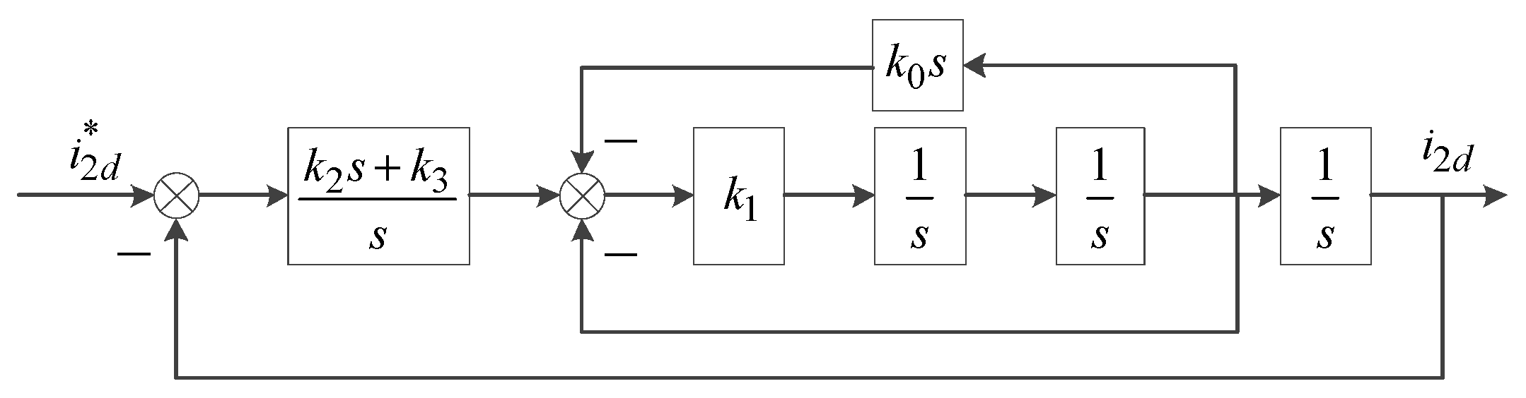
Define the outer loop controller parameters as k2 and k3, the inner loop controller parameter as k1. Then, the control system can be represented as Figure 4.
Open loop and closed loop transfer function of the system can be written as
In the double closed loop current control system shown in (29), the numerator order of the transfer function is quite different from the denominator order. The parameters coupling degree is low. Therefore, the parameters can be designed directly according to the system characteristics. As the parameters design method was analyzed before, this section does not repeat the description.
4. Simulations and Experiments
4.1. Simulation and Experimental Environment
In order to verify the effectiveness of the proposed algorithm, the three-phase static var generator is used as the controlled object.
Matlab/Simulink simulation software (2010b, MathWorks, Inc., Natick, Massachusetts 01760 USA) is used to carry out numerical simulation analysis of three-phase three-leg grid-connected inverter based on feedback linearization. IGBT model in MATLAB/Simulink simulation software is selected as switch, with internal resistance Ron = 1 mΩ, snubber resistance Rs = 500 kΩ, snubber capacitance Cs = inf.
Furthermore, in order to verify the feasibility of the algorithm, a 50 kW prototype of three-phase three-leg inverter is built and the experiment is carried out. The Controller chip of the prototype is TMS320F28335 (Texas Instruments, Inc., Dallas, Texas 75243 USA). The IGBT module is SKM150GB12V (Semikron, Ltd., Nuremberg, Germany), with the switching frequency of 10 kHz.
A photograph of the test rig is shown in Figure 5.
Based on the system parameters shown in Table 1, the control parameters of the two feedback linearized systems are selected, respectively.
- Based on Equations (17)–(20), selecting the cut-off frequency of the open-loop transfer function as 750 Hz, the single closed-loop control system parameters can be designed as: k3 = 5000, k2 = 107π, k1 = 200k2, k0 = 104k2. At this time, the corresponding phase margin is Pm = 45°, and the closed-loop bandwidth is 1 kHz.
- Similarly, the parameters of the double closed loop control system can be designed as: k0 = 2 × 10⁻⁴, k1 = 108, k2 = 5 × 10³, k3 = 102k3. Then, the corresponding open loop cut-off frequency is 680 Hz, phase margin is Pm = 43°, and closed-loop bandwidth is 1 kHz.
The corresponding frequency domain characteristics of two control systems are shown in Figure 6.
4.2. Steady State Control Performance
Setting VSI output current as i2 = 50 A, the three-phase output current on the basis of two control methods is shown in Figure 7.
According to Figure 7, both the two inverter systems can track the reference current accurately with small current distortion. Compared to single closed loop control, the output ripple of double closed loop control system is smaller.
The prototype is adopted to carry out the experiment. The output current of the system based on two kinds of control methods is shown in Figure 8. The output current Total Harmonic Distortion (THD) with the two control methods are 4.36% and 1.57%, respectively. The current ripple of single closed loop control system based on feedback linearization is larger. The main reason is that the control system is highly dependent on the accuracy of the system model. However, the sampling and control delays, which exist in real systems, cause the inaccuracy of the feedback signal. In addition, the nonlinear magnetization curve of the inductance and the equivalent series resistance of the capacitance also affect the model accuracy. It reduces the damping effect of the resonance point and increases the current ripple. The reduced order double closed loop controller takes the filter capacitor voltage as the intermediate variable. To some extent, the measure reduces the coupling relationship among the control variables and improves the robustness of the system. The steady state control performance is better.
4.3. Dynamic Control Performance
In this paper, a dynamic test is carried out in the form of virtual load. The grid-connected current is set as 25 A at the initial time, and then doubles at 0.3 s. The output current of the system is shown in Figure 9.
When the load current changes, the output current of the two systems fluctuates with little overshoot. After a brief transient process, the system reaches a new steady state within one fundamental period. Compared to the direct feedback linearization control, the reduced order feedback linearization control lacks one closed loop zero, which reduces the response speed. However, the transition process is relatively smooth. Therefore, it can be seen that the two control schemes both have fast response and small overshoot.
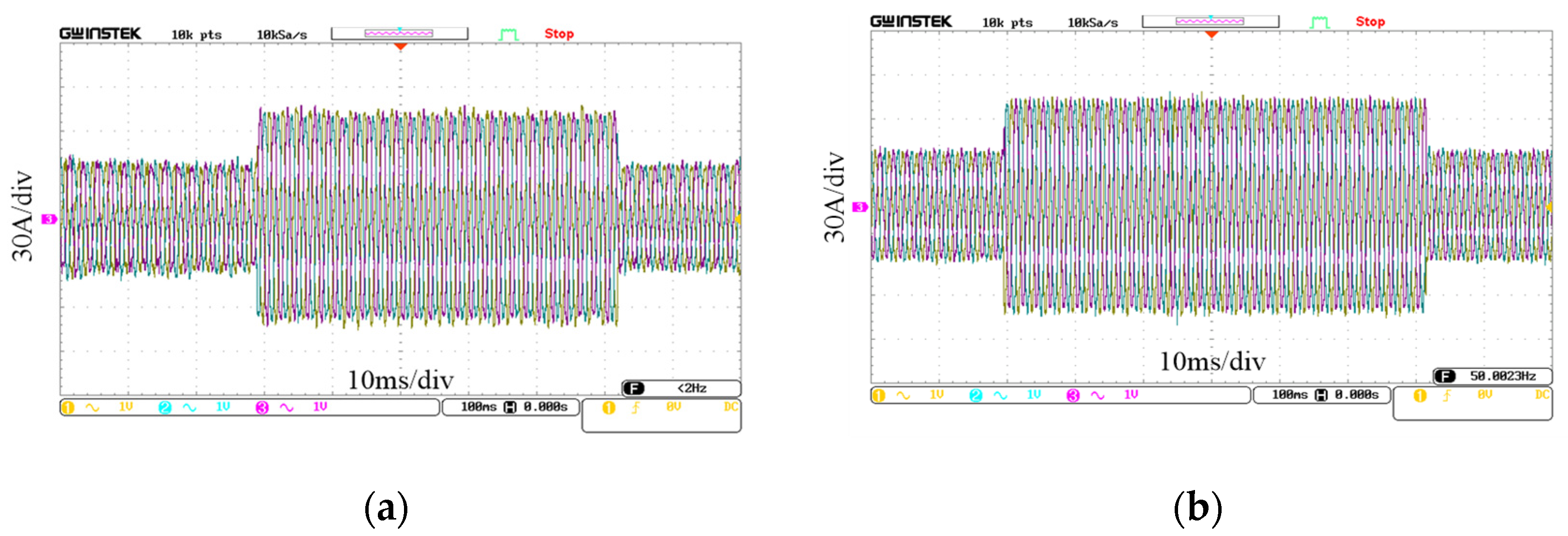
The experimental conditions are the same as those of the simulation. The experimental results are shown in Figure 10. Similar to the simulation results, it is shown that both of the two control schemes have good dynamic performance.
5. Conclusions
In order to solve the problem of poor global control performance of the controller designed by small signal modeling and harmonic linearization, two universal controller design methods based on state feedback linearization are proposed for the LCL type VSI. Relation degree of the VSI system and that of the reduced order model are analyzed, respectively. Subsequently, the coupling matrixes are designed by adopting the Lie derivative. Through the nonlinear transformation, the original system is mapped to the Brunovsky standard type, and the new system linear controller can be used to complete the control of the original complex system. Then, the parameters design ideas of two kinds of controllers are given. The proposed single closed-loop current controller has a simple structure, but it is highly dependent on the exact model of the system. The double closed loop controller sets the filter capacitor voltage as the inner loop control variable, by which a reduced order feedback linearization control can be achieved step by step, to improve the adaptability and robustness of the system. The simulation and experimental results show that the two controllers have good steady-state control performance and dynamic response performance. In practical application, the robustness of linear control system based on reduced-order feedback is better.
Author Contributions
L.Y. wrote the paper and designed the control method; C.F. contributed to the conception of the study and designed the simulation model; J.L. helped to perform the analysis with constructive discussions.
Acknowledgments
This work is supported by the National Natural Science Foundation of China (Grant No. 51607179) and the Fundamental Research Funds for the Central Universities (2017QNB01).
Conflicts of Interest
No potential conflict of interest was reported by the authors.
References
- Farokhian, F.M.; Roosta, A.; Gitizadeh, M. Stability analysis and decentralized control of inverter-based ac microgrid. Prot. Control Mod. Power Syst. 2019, 4, 65–86. [Google Scholar] [CrossRef]
- Yang, H.; Zhang, Y.; Liang, J.; Gao, J.; Walker, P.; Zhang, N. Sliding-mode observer based voltage-sensorless model predictive power control of pwm rectifier under unbalanced grid condition. IEEE Trans. Ind. Electron. 2018, 65, 5550–5560. [Google Scholar] [CrossRef]
- Xu, X.; Casale, E.; Bishop, M. Application guidelines for a new master controller model for statcom control in dynamic analysis. IEEE Trans. Power Deliv. 2017, 32, 2555–2564. [Google Scholar] [CrossRef]
- Bosch, S.; Staiger, J.; Steinhart, H. Predictive current control for an active power filter with lcl-filter. IEEE Trans. Ind. Electron. 2018, 65, 4943–4952. [Google Scholar] [CrossRef]
- Liu, B.; Wei, Q.; Zou, C.; Duan, S. Stability analysis of lcl-type grid-connected inverter under single-loop inverter-side current control with capacitor voltage feedforward. IEEE Trans. Ind. Inform. 2017, 14, 691–702. [Google Scholar] [CrossRef]
- Jamshidifar, A.; Jovcic, D. Small-signal dynamic dq model of modular multilevel converter for system studies. IEEE Trans. Power Deliv. 2016, 31, 191–199. [Google Scholar] [CrossRef]
- Bao, X.; Zhuo, F.; Tian, Y.; Tan, P. Simplified feedback linearization control of three-phase photovoltaic inverter with an lcl filter. IEEE Trans. Power Electron. 2013, 28, 2739–2752. [Google Scholar] [CrossRef]
- Lamperski, A.; Ames, A.D. Lyapunov theory for zeno stability. IEEE Trans. Autom. Control 2012, 58, 100–112. [Google Scholar] [CrossRef]
- Hwang, C.L.; Fang, W.L. Global fuzzy adaptive hierarchical path tracking control of a mobile robot with experimental validation. IEEE Trans. Fuzzy Syst. 2016, 24, 724–740. [Google Scholar] [CrossRef]
- Kim, D.E.; Lee, D.C. Feedback linearization control of three-phase ups inverter systems. IEEE Trans. Ind. Electron. 2010, 57, 963–968. [Google Scholar]
- Akhtar, A.; Nielsen, C.; Waslander, S.L. Path following using dynamic transverse feedback linearization for car-like robots. IEEE Trans. Robot. 2017, 31, 269–279. [Google Scholar] [CrossRef]
- Choi, Y.S.; Han, H.C.; Jung, J.W. Feedback linearization direct torque control with reduced torque and flux ripples for ipmsm drives. IEEE Trans. Power Electron. 2015, 31, 3728–3737. [Google Scholar] [CrossRef]
- Yang, L.Y.; Liu, J.H.; Wang, C.L.; Du, G.F. Sliding mode control of three-phase four-leg inverters via state feedback. J. Power Electron. 2014, 14, 1028–1037. [Google Scholar] [CrossRef]
- Lascu, C.; Jafarzadeh, S.; Fadali, S.M.; Blaabjerg, F. Direct torque control with feedback linearization for induction motor drives. IEEE Trans. Power Electron. 2016, 32, 2072–2080. [Google Scholar] [CrossRef]
- Yang, S.; Wang, P.; Tang, Y. Feedback linearization based current control strategy for modular multilevel converters. IEEE Trans. Power Electron. 2017, 33, 161–174. [Google Scholar]
Figure 1.
Schematic diagram of the three-phase three-leg grid-connected inverter.
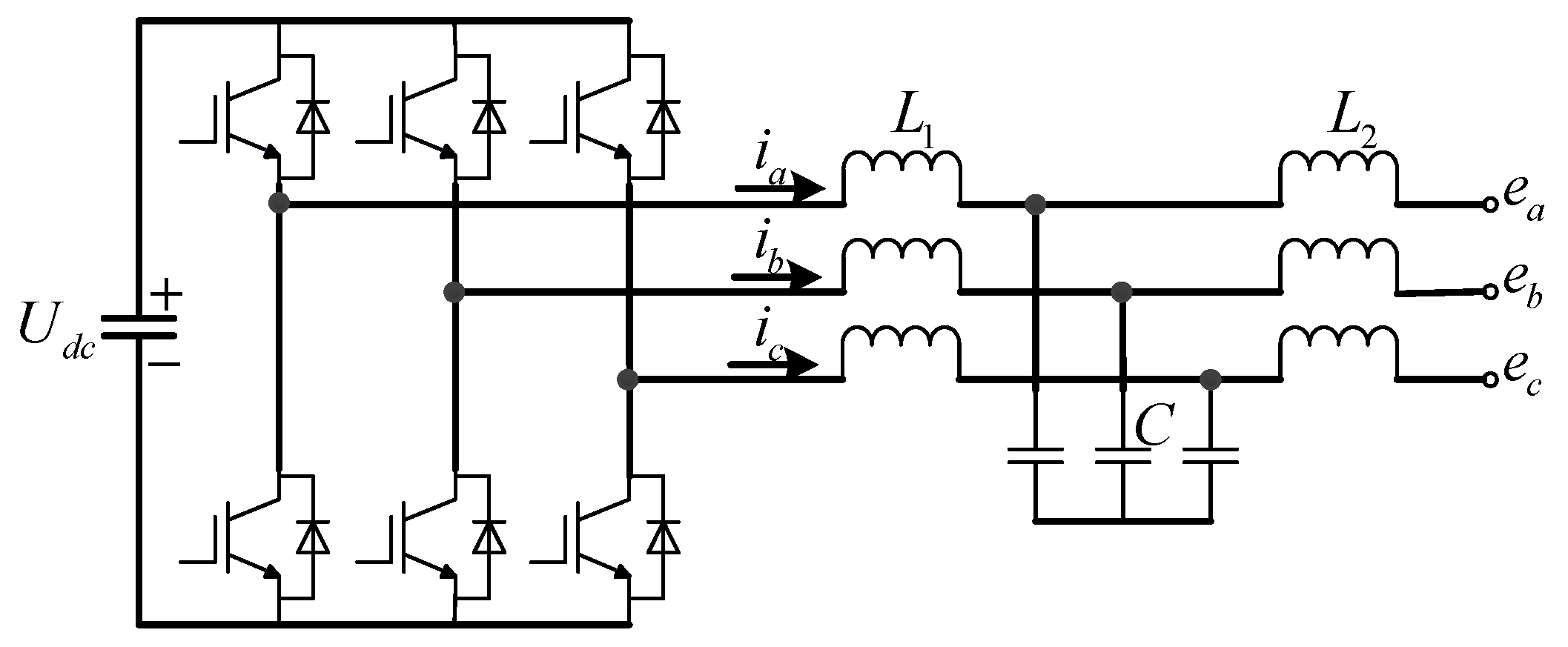
Figure 2.
Current control system based on state feedback linearization.
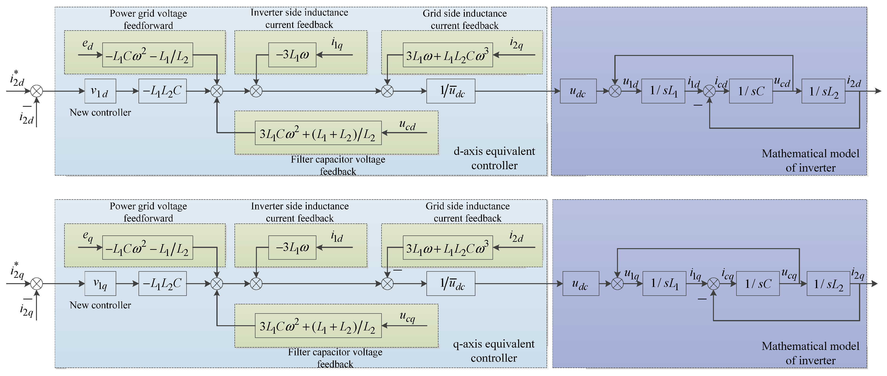
Figure 3.
Block diagram of the reduced order feedback decoupling control system.
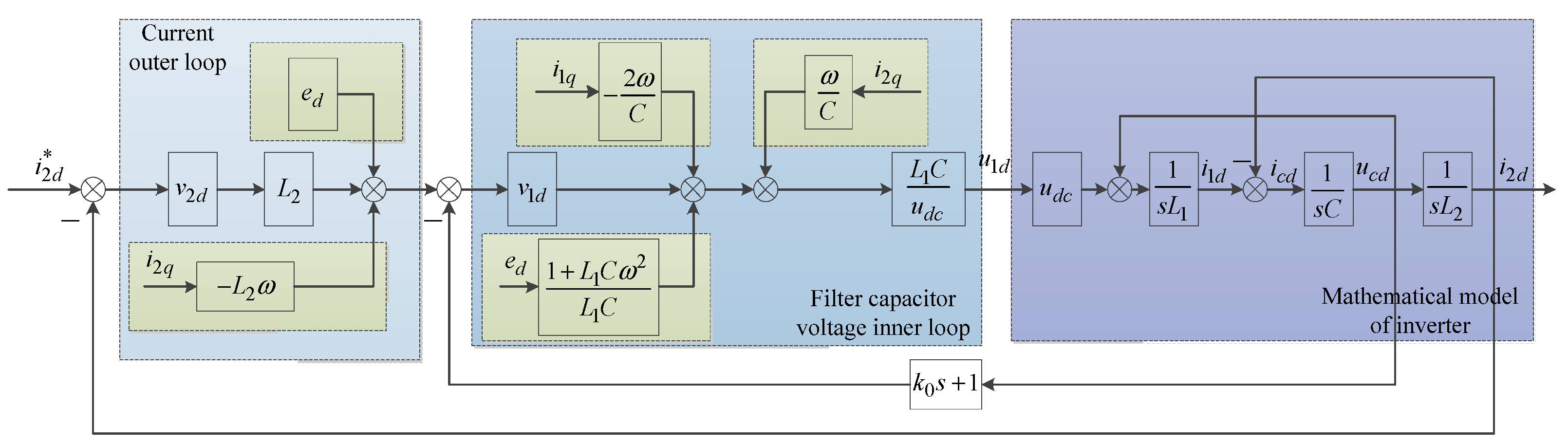
Figure 4.
Equivalent block diagram of control system.

Figure 5.
Photograph of the experimental test rig.
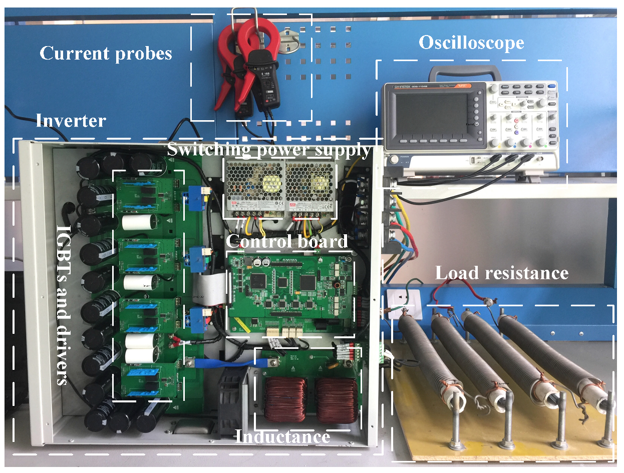
Figure 6.
Bode diagrams of the closed-loop control systems: (a) Single closed-loop control system, (b) double closed-loop control system.
Figure 6.
Bode diagrams of the closed-loop control systems: (a) Single closed-loop control system, (b) double closed-loop control system.
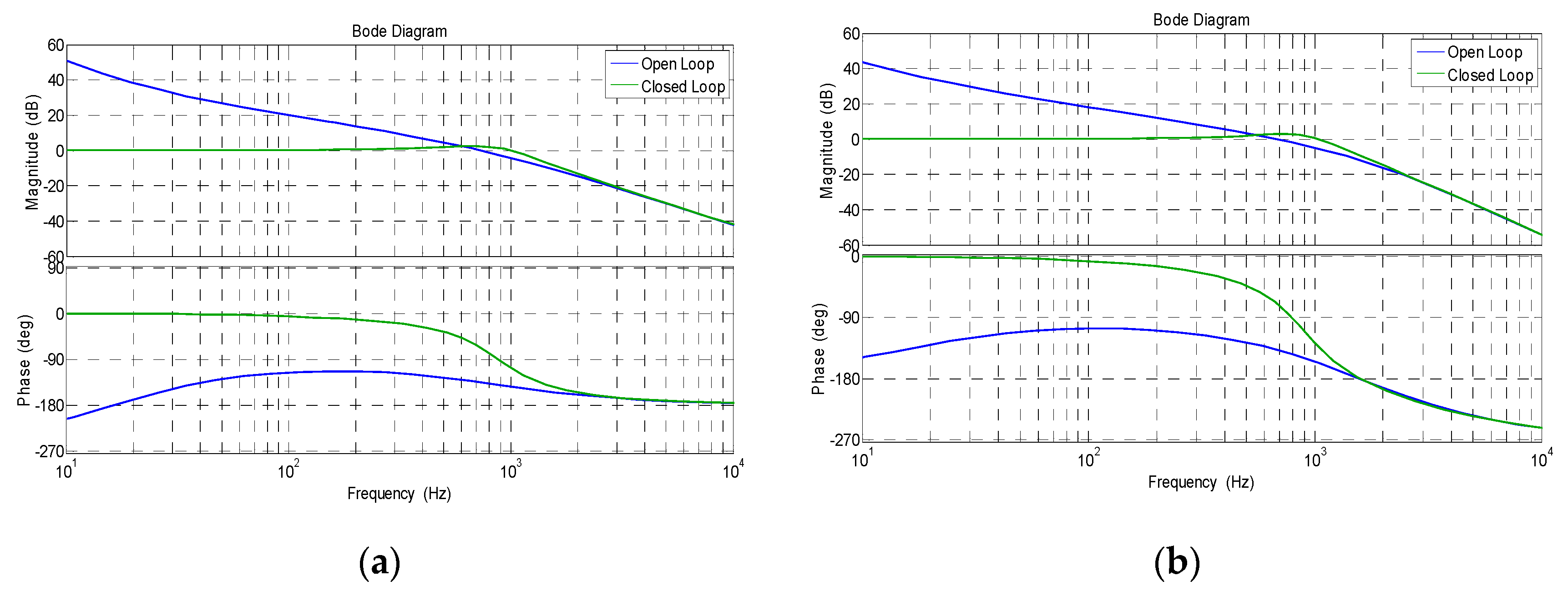
Figure 7.
Steady-state current waveforms of voltage source inverters (VSI) based on two control schemes: (a) Output current of the single closed-loop control system, (b) output current of the double closed-loop control system.
Figure 7.
Steady-state current waveforms of voltage source inverters (VSI) based on two control schemes: (a) Output current of the single closed-loop control system, (b) output current of the double closed-loop control system.
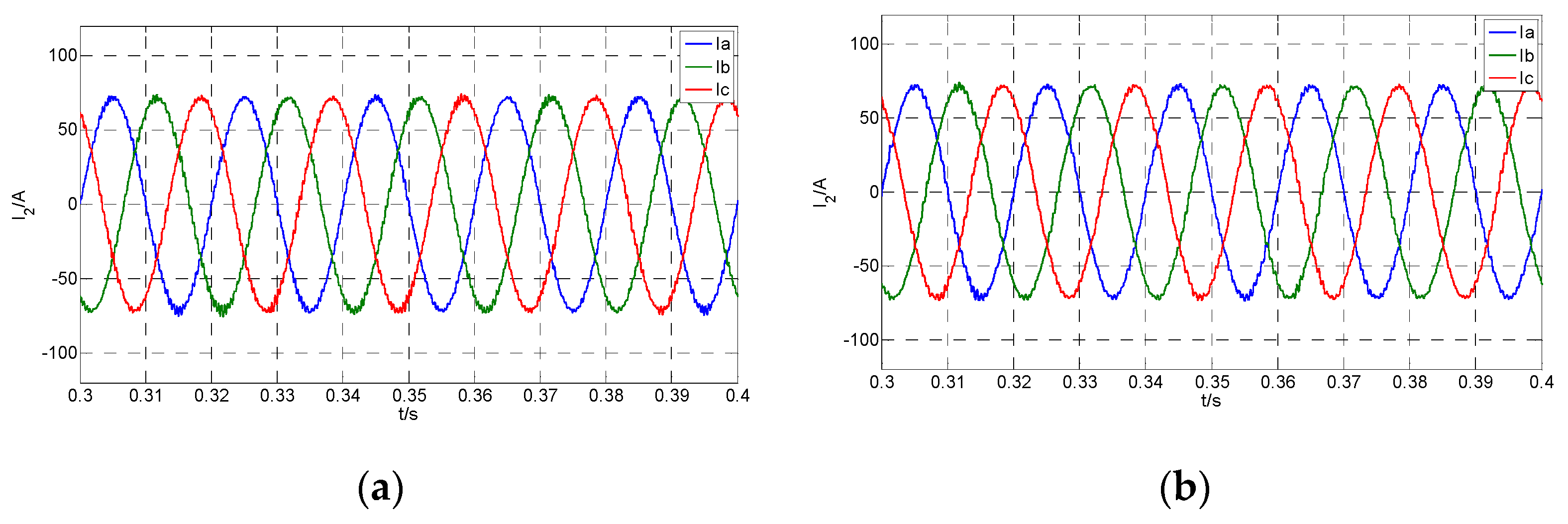
Figure 8.
Experimental steady-state current waveforms: (a) Output current of the single closed-loop control experiment, (b) output current of the double closed-loop control experiment.
Figure 8.
Experimental steady-state current waveforms: (a) Output current of the single closed-loop control experiment, (b) output current of the double closed-loop control experiment.
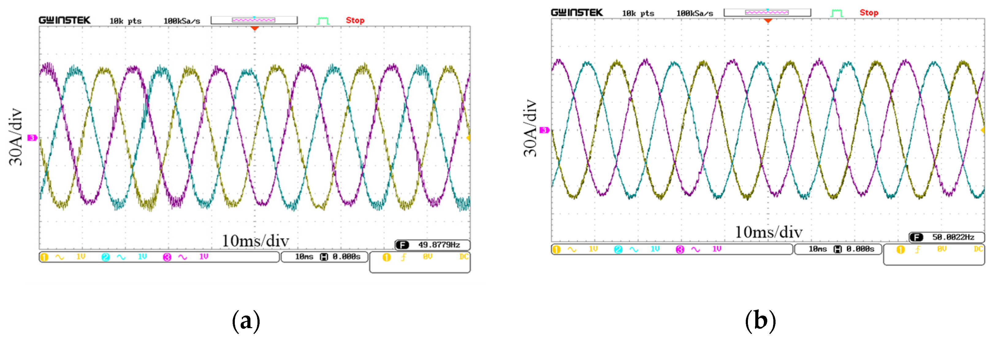
Figure 9.
Dynamic current waveforms of VSI based on two control schemes: (a) Output current of the single closed-loop control system, (b) output current of the double closed-loop control system, (c) partial enlarged detail of (a), (d) partial enlarged detail of (b).
Figure 9.
Dynamic current waveforms of VSI based on two control schemes: (a) Output current of the single closed-loop control system, (b) output current of the double closed-loop control system, (c) partial enlarged detail of (a), (d) partial enlarged detail of (b).
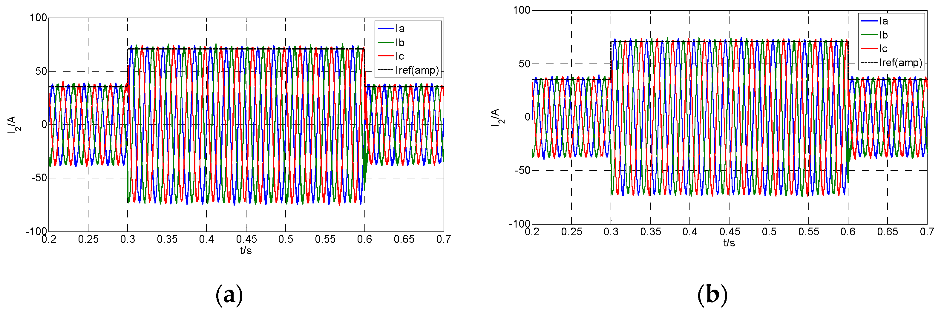

Figure 10.
Experimental dynamic current waveforms: (a) Output current of the single closed-loop control experiment, (b) output current of the double closed-loop control experiment.
Figure 10.
Experimental dynamic current waveforms: (a) Output current of the single closed-loop control experiment, (b) output current of the double closed-loop control experiment.

Table 1.
Parameters for the system.
| Variables | Symbols | Value |
|---|---|---|
| DC Bus Voltage | udc | 650 V |
| Grid Voltage | ug | 380 V |
| Grid-side inductor | L2 | 0.2 mH |
| Inverter side inductor | L1 | 0.3 mH |
| Filter capacitor | C | 20 uF |
| Switching frequency | f | 10 kHz |
© 2019 by the authors. Licensee MDPI, Basel, Switzerland. This article is an open access article distributed under the terms and conditions of the Creative Commons Attribution (CC BY) license (http://creativecommons.org/licenses/by/4.0/).
Share and Cite
MDPI and ACS Style
Yang, L.; Feng, C.; Liu, J. Control Design of LCL Type Grid-Connected Inverter Based on State Feedback Linearization. Electronics 2019, 8, 877. https://doi.org/10.3390/electronics8080877
AMA Style
Yang L, Feng C, Liu J. Control Design of LCL Type Grid-Connected Inverter Based on State Feedback Linearization. Electronics. 2019; 8(8):877. https://doi.org/10.3390/electronics8080877
Chicago/Turabian StyleYang, Longyue, Chunchun Feng, and Jianhua Liu. 2019. "Control Design of LCL Type Grid-Connected Inverter Based on State Feedback Linearization" Electronics 8, no. 8: 877. https://doi.org/10.3390/electronics8080877
Note that from the first issue of 2016, this journal uses article numbers instead of page numbers. See further details here.