Multivariate Temporal Convolutional Network: A Deep Neural Networks Approach for Multivariate Time Series Forecasting


Abstract
:1. Introduction
2. Background
3. Methodology
3.1. Sequence Problem Statement
3.2. Baseline Test
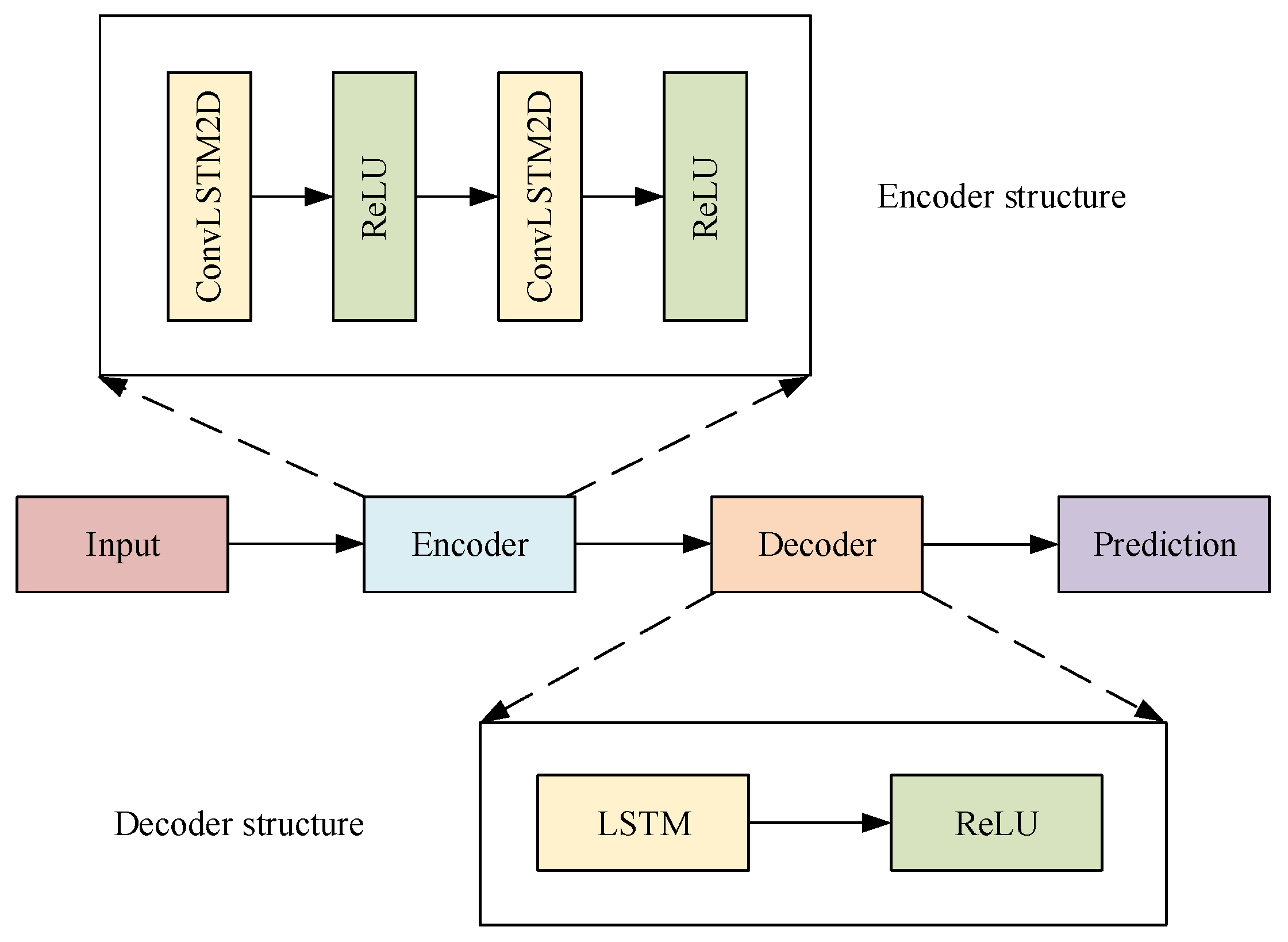
3.3. ConvLSTM Encoder–Decoder Model
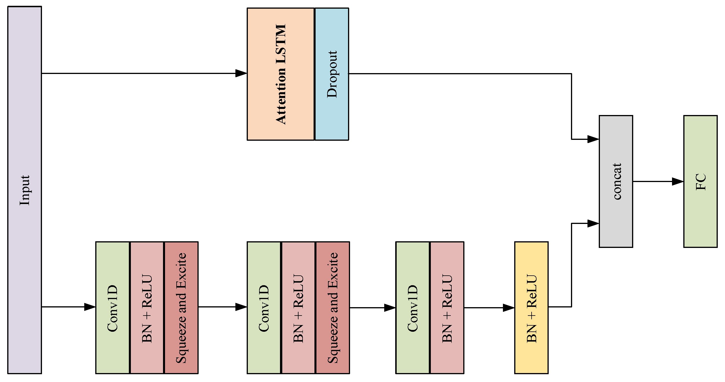
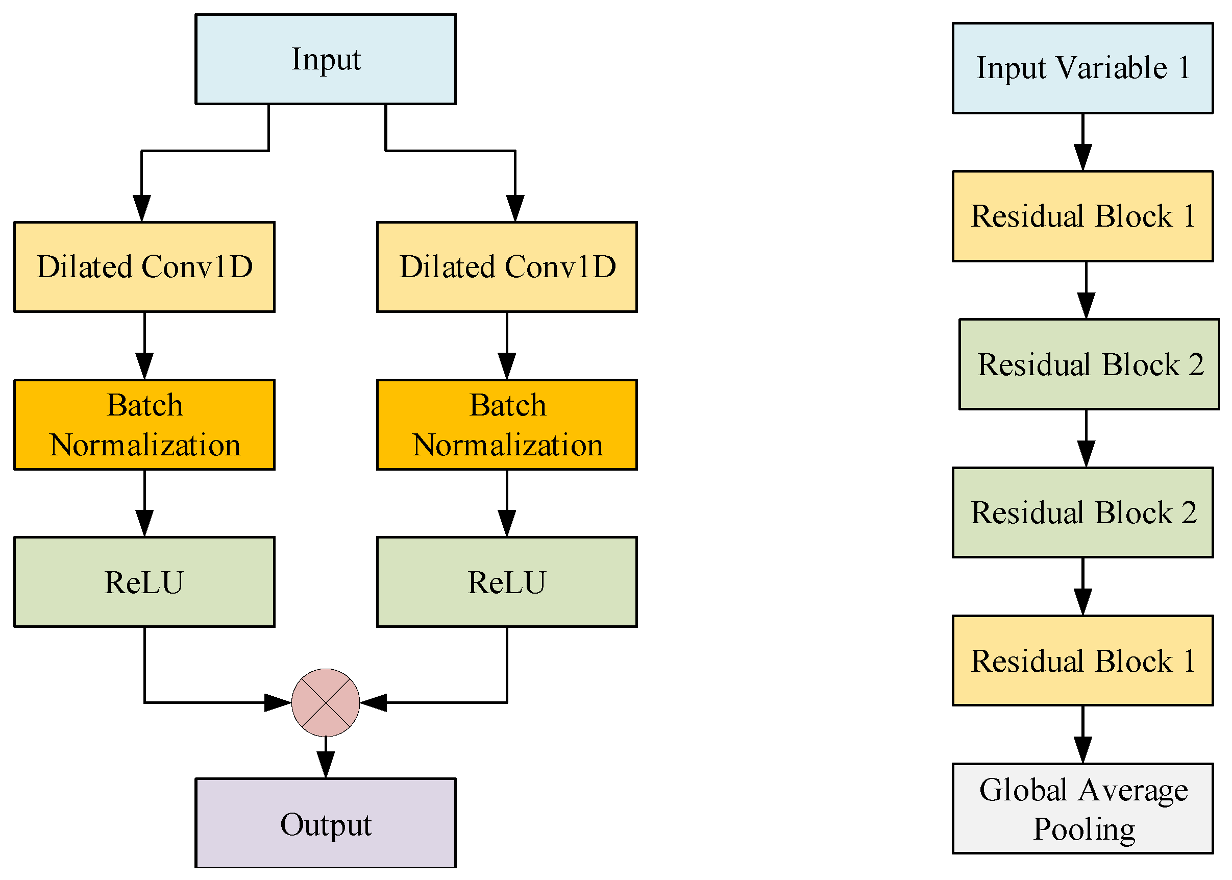
3.4. M-TCN Model
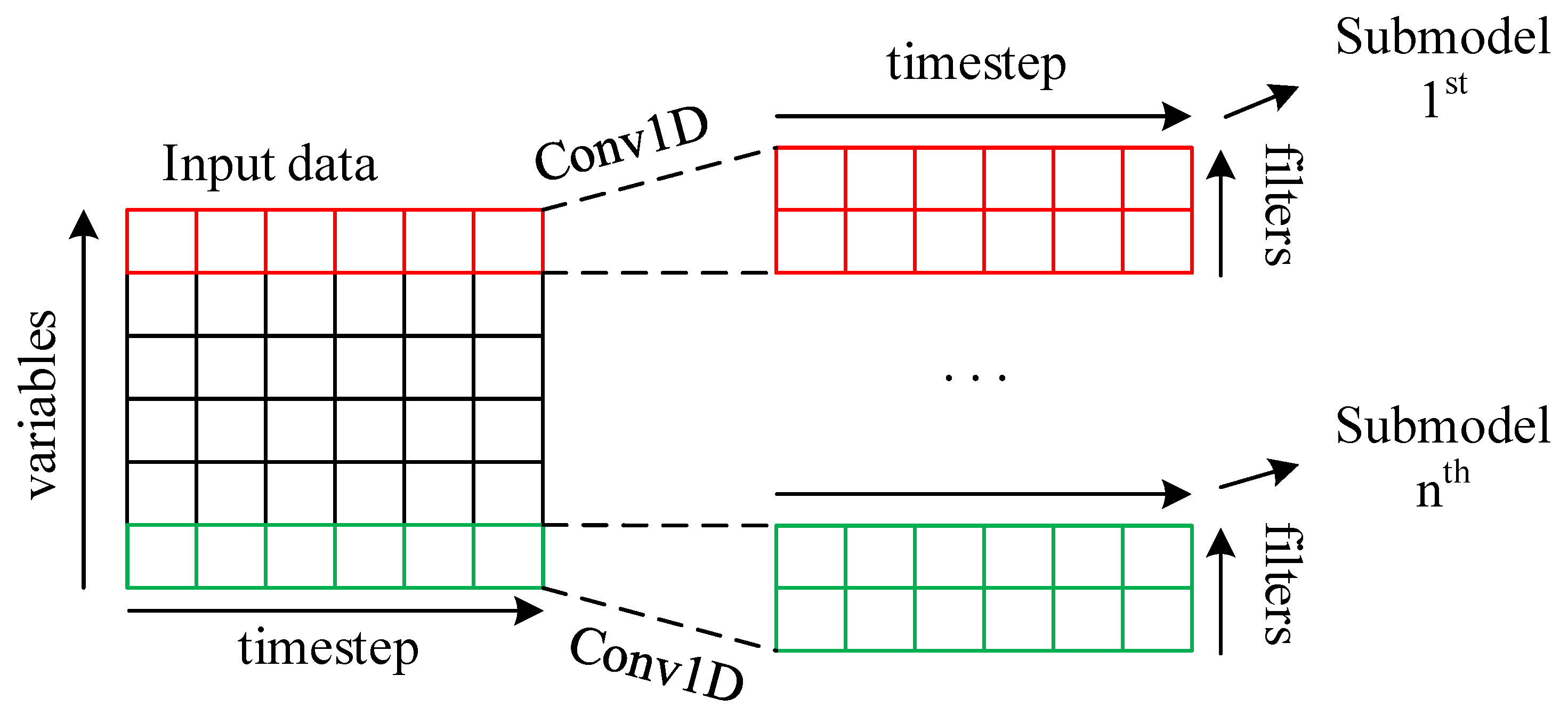
3.4.1. 1D Convolutions
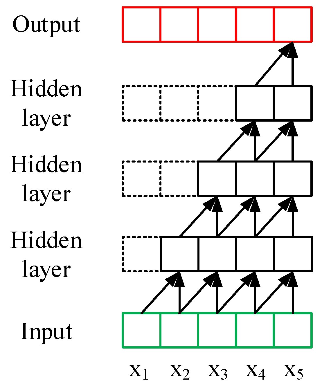
3.4.2. Dilated Convolutions
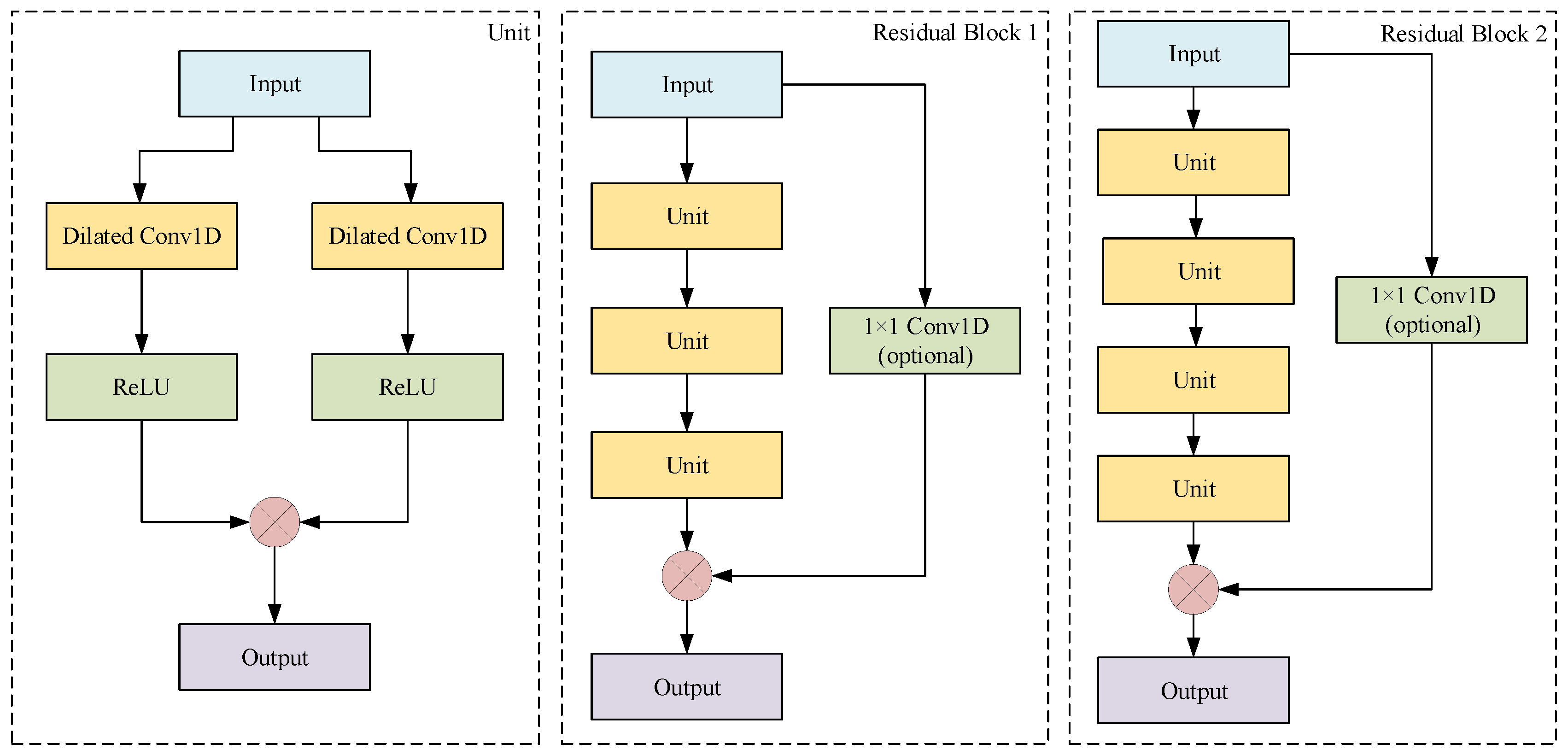
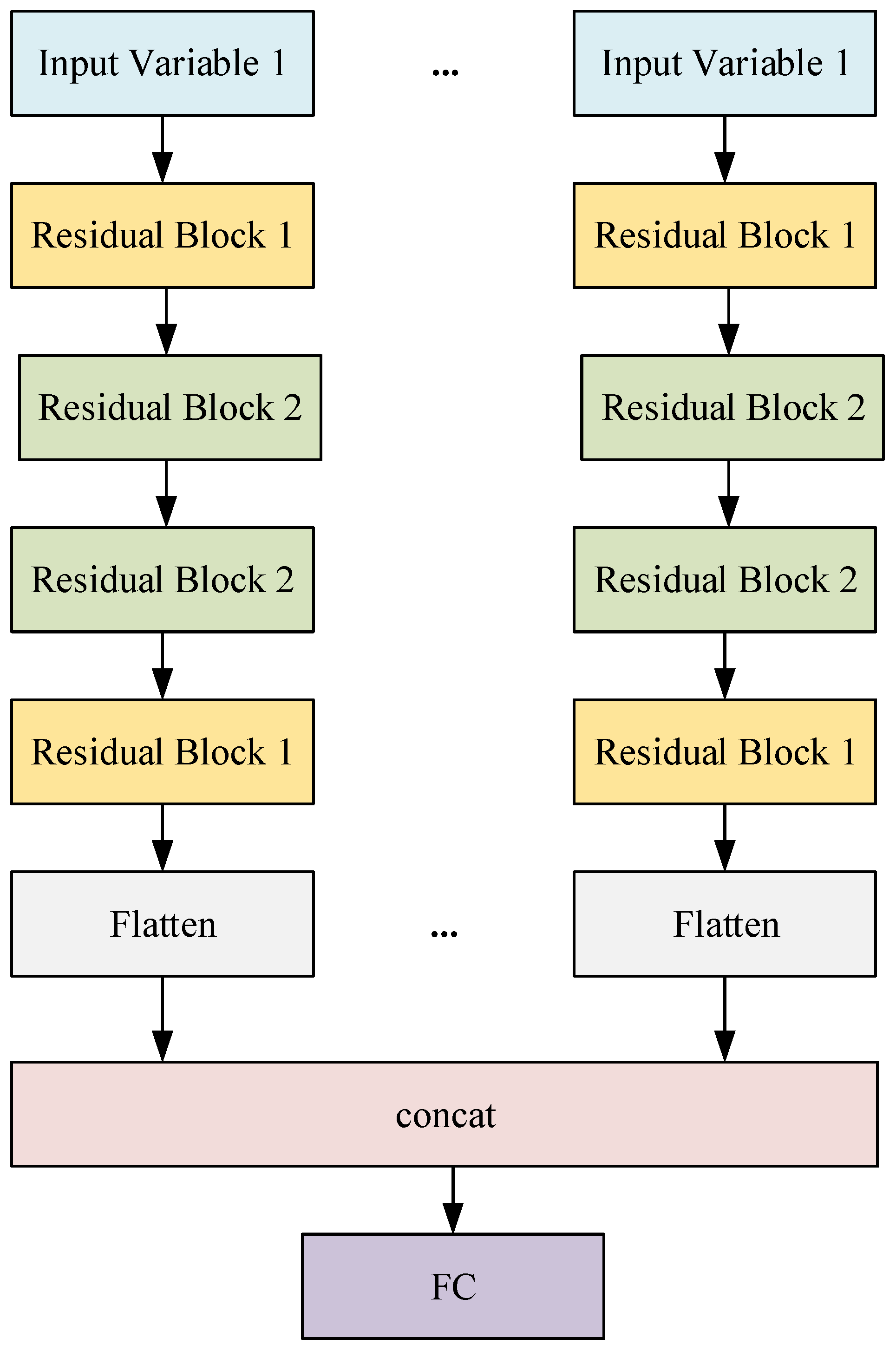
3.4.3. Residual Block
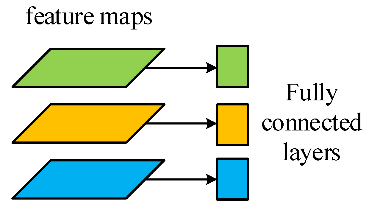
3.4.4. Fully Connected Layers
3.4.5. Multi-Head Model
3.5. Training Procedure
| Algorithm 1: Training procedure. |
|
4. Experiments
4.1. Datasets
4.2. Data Processing
4.3. Evaluation Criteria
4.4. Walk-Forward Validation
- Step 1: Starting at the beginning of the test set, the last set of observations in the training set is used as input of the model to predict the next set of data (the first set of true values in the validation set).
- Step 2: The model makes a prediction for the next time step.
- Step 3: Get real observation and add to history for predicting the next time.
- Step 4: The prediction is stored and evaluated against the real observation.
- Step 5: Go to step 1.
4.5. Experimental Details
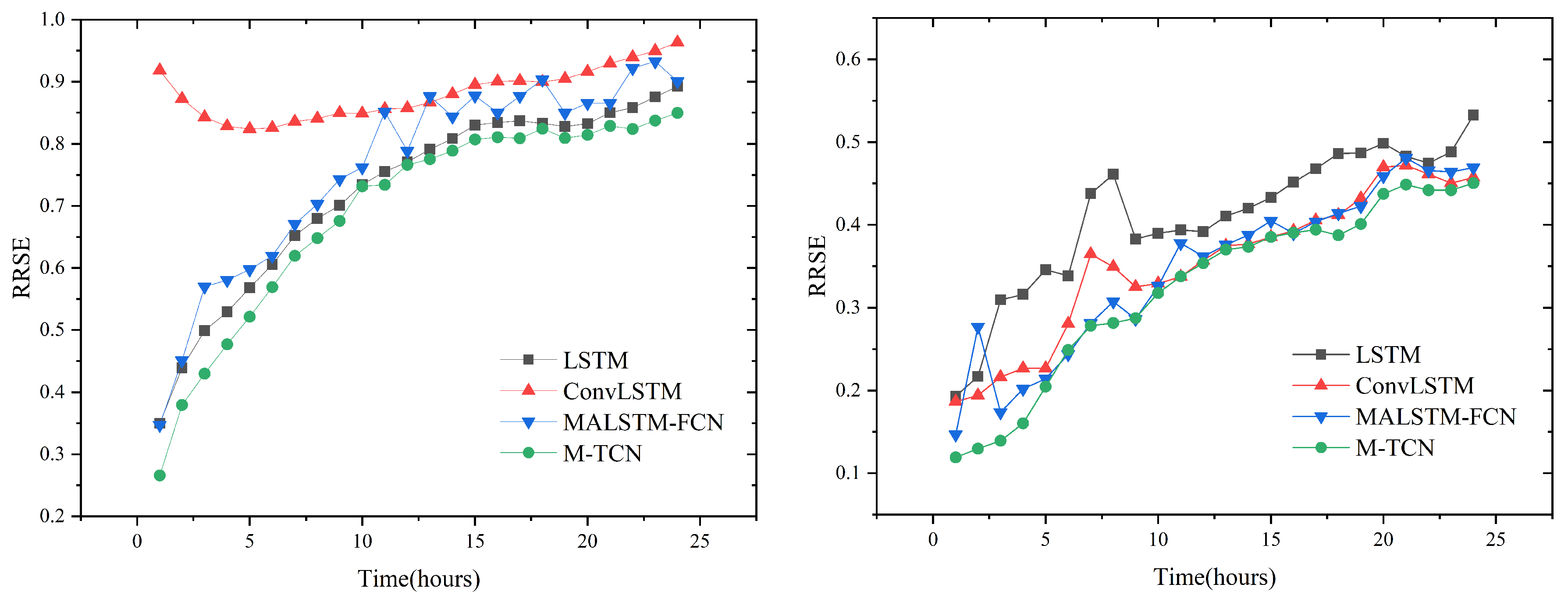
4.6. Experimental Results
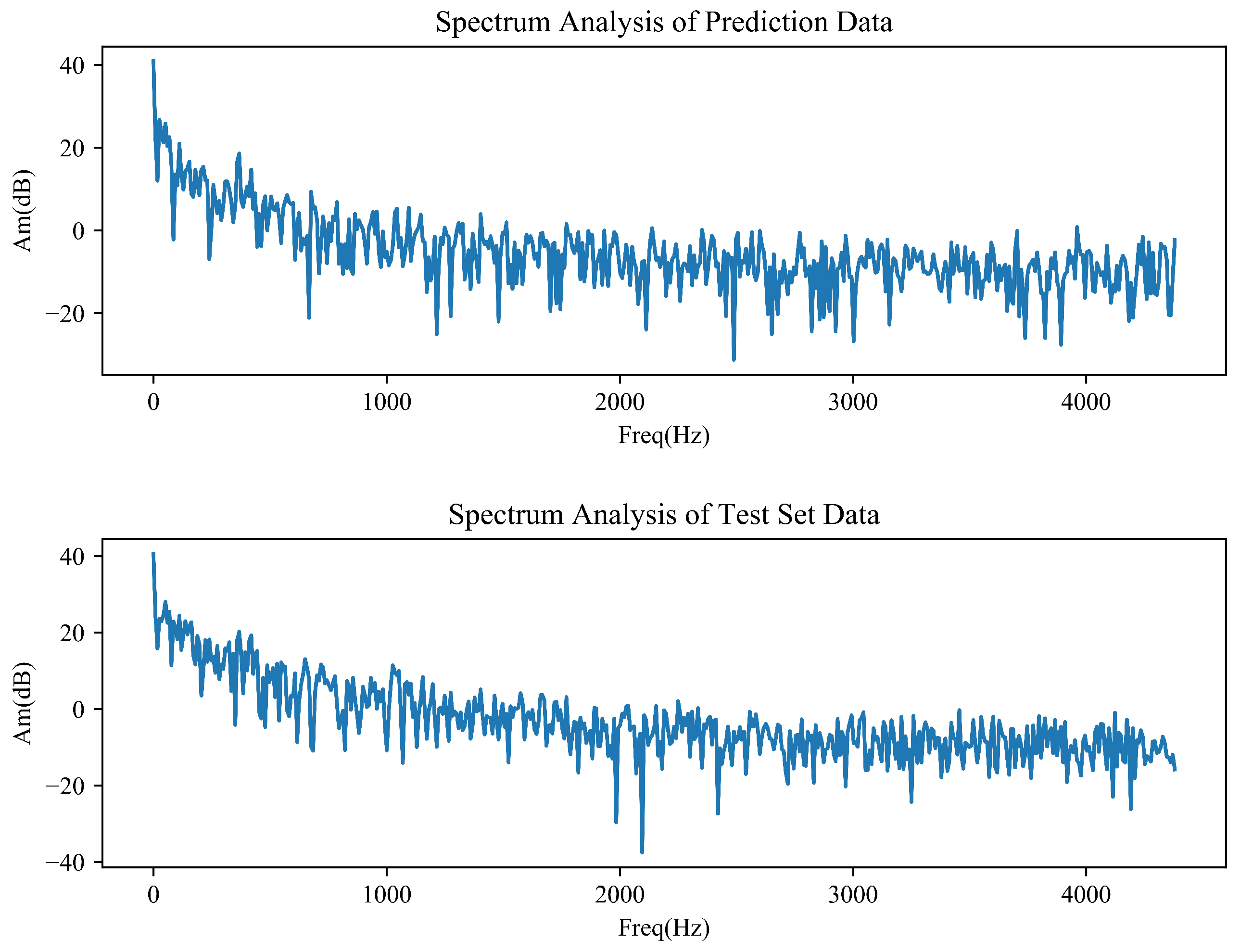
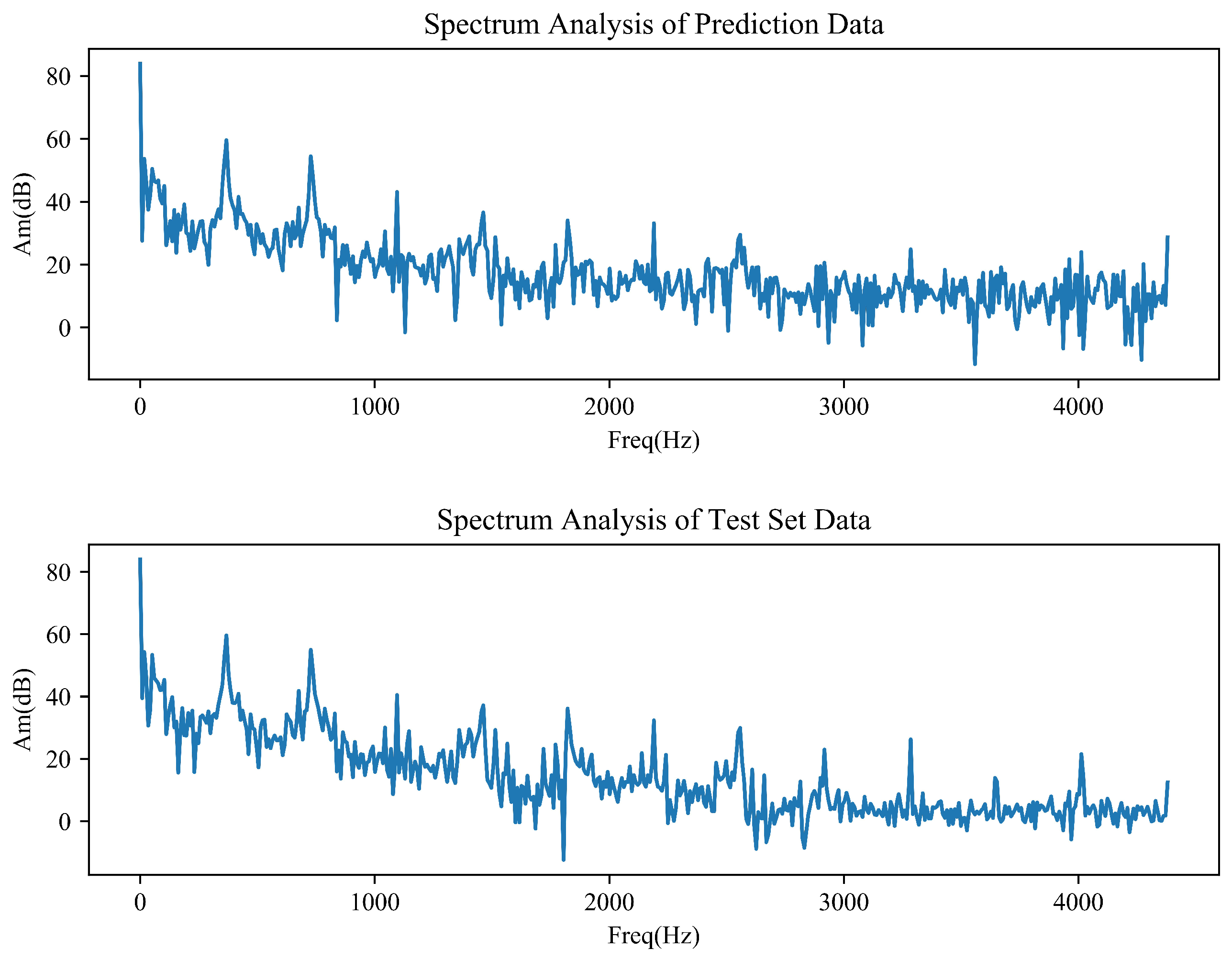
4.7. Spectrum Analysis
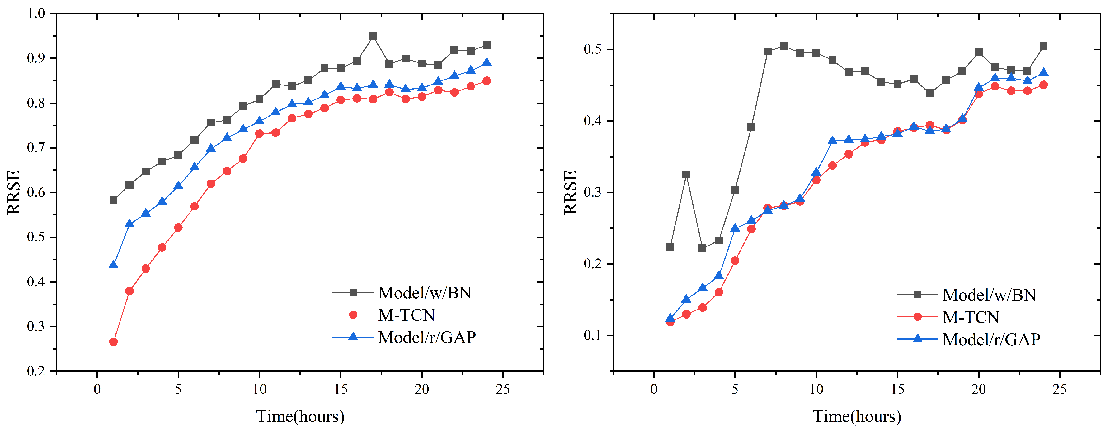
4.8. Ablation Tests
4.9. Model Efficiency
5. Conclusions
Author Contributions
Funding
Conflicts of Interest
References
- Seyed, B.L.; Behrouz, M. Comparison between ANN and Decision Tree in Aerology Event Prediction. In Proceedings of the International Conference on Advanced Computer Theory & Engineering, Phuket, Thailand, 20–22 December 2008; pp. 533–537. [Google Scholar] [CrossRef]
- Simmonds, J.; Gómez, J.A.; Ledezma, A. Data Preprocessing to Enhance Flow Forecasting in a Tropical River Basin. In Engineering Applications of Neural Networks; Springer: Cham, Switzerland, 2017; pp. 429–440. [Google Scholar]
- Mohamad, S. Artificial intelligence for the prediction of water quality index in groundwater systems. Model. Earth Syst. Environ. 2016, 2, 8. [Google Scholar]
- Amato, F.; Castiglione, A.; Moscato, V.; Picariello, A.; Sperlì, G. Multimedia summarization using social media content. Multimed. Tools Appl. 2018, 77, 17803–17827. [Google Scholar] [CrossRef]
- Kadir, K.; Halim, C.; Harun, K.O.; Olcay, E.C. Modeling and prediction of Turkey’s electricity consumption using Artificial Neural Networks. Energy Convers. Manag. 2009, 50, 2719–2727. [Google Scholar]
- Wu, Y.; José, M.H.; Ghahramani, Z. Dynamic Covariance Models for Multivariate Financial Time Series. arXiv 2013, arXiv:1305.4268. [Google Scholar]
- Yu, R.; Li, Y.; Shahabi, C.; Demiryurek, U.; Liu, Y. Deep learning: A generic approach for extreme condition traffic forecasting. In Proceedings of the 2017 SIAM International Conference on Data Mining, Houston, TX, USA, 27–29 April 2017; pp. 777–785. [Google Scholar]
- Akaike, H. Fitting autoregressive models for prediction. Ann. Inst. Stat. Math. 1969, 21, 243–247. [Google Scholar] [CrossRef]
- Frigola, R.; Rasmussen, C.E. Integrated pre-processing for bayesian nonlinear system identification with gaussian processes. In Proceedings of the IEEE Conference on Decision and Control, Florence, Italy, 10–13 December 2013; pp. 552–560. [Google Scholar]
- Alom, M.; Tha, T.; Yakopcic, C.; Westberg, S.; Sidike, P.; Nasrin, M.; Hasan, M.; Essen, B.; Awwal, A.; Asari, V. A State-of-the-Art Survey on Deep Learning Theory and Architectures. Electronics 2019, 8, 292. [Google Scholar] [CrossRef]
- Liu, L.; Finch, A.M.; Utiyama, M.; Sumita, E. Agreement on Target-Bidirectional LSTMs for Sequence-to-Sequence Learning. In Proceedings of the Thirtieth Aaai Conference on Artificial Intelligence, Phoenix, AZ, USA, 12–17 February 2016; pp. 2630–2637. [Google Scholar]
- Gehring, J.; Auli, M.; Grangier, D.; Yarats, D.; Dauphin, Y.N. Convolutional Sequence to Sequence Learning. arXiv 2017, arXiv:1705.03122. [Google Scholar]
- Yu, F.; Koltun, V.; Funkhouser, T. Dilated Residual Networks. In Proceedings of the IEEE Conference on Computer Vision and Pattern Recognition (CVPR), Honolulu, HI, USA, 21–26 July 2017; pp. 472–480. [Google Scholar] [CrossRef]
- He, K.; Zhang, X.; Ren, S.; Sun, J. Deep Residual Learning for Image Recognition. In Proceedings of the IEEE Conference on Computer Vision and Pattern Recognition (CVPR), Las Vegas, NV, USA, 26 June–1 July 2016; pp. 770–778. [Google Scholar] [CrossRef]
- Ediger, V.; Akar, S. ARIMA forecasting of primary energy demand by fuel in Turkey. Energy Policy 2007, 35, 1701–1708. [Google Scholar] [CrossRef]
- Rojas, I.; Valenzuela, O.; Rojas, F.; Guillen, A.; Herreraet, L.; Pomares, H.; Marquez, L.; Pasadas, M. Soft-computing techniques and ARMA model for time series prediction. Neurocomputing 2008, 71, 519–537. [Google Scholar] [CrossRef]
- Kilian, L. New introduction to multiple time series analysis. Econ. Rec. 2006, 83, 109–110. [Google Scholar]
- Sapankevych, N.; Sankar, R. Time Series Prediction Using Support Vector Machines: A Survey. IEEE Comput. Intell. Mag. 2009, 4, 24–38. [Google Scholar] [CrossRef]
- Hamidi, O.; Tapak, L.; Abbasi, H.; Abbasi, H.; Maryanaji, Z. Application of random forest time series, support vector regression and multivariate adaptive regression splines models in prediction of snowfall (a case study of Alvand in the middle Zagros, Iran). Theor. Appl. Climatol. 2018, 134, 769–776. [Google Scholar] [CrossRef]
- Lima, C.; Lall, U. Climate informed monthly streamflow forecasts for the Brazilian hydropower network using a periodic ridge regression model. J. Hydrol. 2010, 380, 438–449. [Google Scholar] [CrossRef]
- Li, J.; Chen, W. Forecasting macroeconomic time series: LASSO-based approaches and their forecast combinations with dynamic factor models. Int. J. Forecast. 2014, 30, 996–1015. [Google Scholar] [CrossRef]
- Hochreiter, S.; Schmidhuber, J. Long Short-Term Memory. Neural Comput. 1997, 9, 1735–1780. [Google Scholar] [CrossRef]
- Shi, X.; Chen, Z.; Wang, H.; Yeung, D.Y.; Wong, W.K.; Woo, W.C. Convolutional LSTM Network: A Machine Learning Approach for Precipitation Nowcasting. In Proceedings of the Neural Information Processing Systems Conference, Montreal, QC, Canada, 7–12 December 2015; pp. 802–810. [Google Scholar]
- Karim, F.; Majumdar, S.; Darabi, H.; Harforda, S. Multivariate LSTM-FCNs for Time Series Classification. Neural Netw. 2019, 116, 237–245. [Google Scholar] [CrossRef]
- Huang, N.E.; Zheng, S.; Long, S.R.; Wu, M.C.; Shih, H.H.; Zheng, Q.; Yen, N.-C.; Tung, C.C.; Liu, H.H. The empirical mode decomposition and the Hilbert spectrum for nonlinear and non-stationary time series analysis. Proc. Math. Phys. Eng. Sci. 1998, 454, 903–995. [Google Scholar] [CrossRef]
- Wu, Z.; Huang, N.E. Ensemble empirical mode decomposition: A noise-assisted data analysis method. Adv. Adapt. Data Anal. 2009, 1, 1–41. [Google Scholar] [CrossRef]
- Wang, J.; Wang, Z.; Li, J.; Wu, J. Multilevel Wavelet Decomposition Network for Interpretable Time Series Analysis. In Proceedings of the 24th ACM SIGKDD International Conference, London, UK, 19–23 August 2018; pp. 2437–2446. [Google Scholar] [CrossRef]
- Dragomiretskiy, K.; Zosso, D. Variational Mode Decomposition. IEEE Trans. Signal Process. 2014, 62, 531–544. [Google Scholar] [CrossRef]
- Bai, S.; Kolter, J.Z.; Koltun, V. An Empirical Evaluation of Generic Convolutional and Recurrent Networks for Sequence Modeling. arXiv 2018, arXiv:1803.01271. [Google Scholar]
- Dou, C.; Zheng, Y.; Yue, D.; Zhang, Z.; Ma, K. Hybrid model for renewable energy and loads prediction based on data mining and variational mode decomposition. IET Gener. Transm. Distrib. 2018, 12, 2642–2649. [Google Scholar] [CrossRef]
- Howard, A.; Sandler, M.; Chu, G.; Chen, L.-C.; Chen, B.; Tan, M.; Wang, W.; Zhu, Y.; Pang, R.; Vasudevan, V.; et al. Searching for MobileNetV3. arXiv 2018, arXiv:1905.02244. [Google Scholar]
- Cai, H.; Zhu, L.; Han, S. ProxylessNAS: Direct Neural Architecture Search on Target Task and Hardware. arXiv 2018, arXiv:1812.00332. [Google Scholar]
- Elsken, T.; Metzen, J.H.; Hutter, F. Neural Architecture Search: A Survey. arXiv 2018, arXiv:1808.05377. [Google Scholar]
- Nair, V.; Hinton, G. Rectified linear units improve restricted Boltzmann machines. In Proceedings of the 27th International Conference on International Conference on Machine Learning, Haifa, Israel, 21–24 June 2010; pp. 807–814. [Google Scholar]
- Kingma, D.; Ba, J. Adam:A method for stochastic optimization. arXiv 2014, arXiv:1412.6980. [Google Scholar]
- Sutskever, I.; Martens, J.; Dahl, G.E.; Hinton, G. On the importance of initialization and momentum in deep learning. In Proceedings of the 30th International Conference on International Conference on Machine Learning, Atlanta, GA, USA, 16–21 June 2013; pp. 1139–1147. [Google Scholar]
- Ioffe, S.; Szegedy, C. Batch normalization: Accelerating deep network training by reducing internal covariate. In Proceedings of the 32nd International Conference on Machine Learning, Lille, France, 6–11 July 2015; pp. 448–456. [Google Scholar]


| Method | Advantages | Challenges |
|---|---|---|
| AUTOREGRESSIVE [8] | Simple and efficient for lower order models | Nonlinear, multivariable and non-stationary |
| SVR [18] | Nonlinear and high-dimensional | Selection of free parameters, NOT suitable for big data |
| Hybrid VMD and ANN [30] | Strong explanatory power of mathematics | Pre-processing is complex, poor generalization ability |
| LSTM [22] | mixture of long- and short-term memory | Huge computing resource |
| TCN [29] | Large scale parallel computing mitigating the gradient of explosion and greater flexibility in model structure | Long-term memory |
| Datasets | Length of Time Series | Total Number of Variables | Sample Rate |
|---|---|---|---|
| ISO-NE | 103,776 | 2 | 1 h |
| Beijing PM2.5 | 43,824 | 8 | 1 h |
| Input (Actual Value) | Output (Predicted Value) |
|---|---|
| Current 24 h | Next, 24 h |
| 1d 1 h–1 d 24 h | 2 d 1 h–2 d 24 h |
| 2d 1 h–1 d 24 h | 3 d 1 h–2 d 24 h |
| … | … |
| Methods | Metrics | Beijing PM2.5 Dataset | ISO-NE Dataset |
|---|---|---|---|
| Length = 24 | Length = 24 | ||
| Naive | RMSE | 80.55 | 2823.35 |
| RRSE | 0.8608 | 1.0526 | |
| CORR | 0.6736 | 0.5330 | |
| Average | RMSE | 87.89 | 2363.07 |
| RRSE | 0.9393 | 0.8810 | |
| CORR | 0.4972 | 0.4885 | |
| Seasonal Persistent | RMSE | 123.45 | 1654.38 |
| RRSE | 1.3193 | 0.6168 | |
| CORR | 0.1722 | 0.8314 | |
| LSTM | RMSE | 68.07 | 783.90 |
| RRSE | 0.7275 | 0.2923 | |
| CORR | 0.6877 | 0.9573 | |
| ConvLSTM | RMSE | 82.32 | 687.17 |
| RRSE | 0.8798 | 0.2562 | |
| CORR | 0.4873 | 0.9670 | |
| TCN | RMSE | 112.35 | 720.12 |
| RRSE | 1.1453 | 0.2685 | |
| CORR | 0.0075 | 0.9636 | |
| MALSTM-FCN | RMSE | 71.54 | 680.95 |
| RRSE | 0.7646 | 0.2539 | |
| CORR | 0.6463 | 0.9677 | |
| M-TCN | RMSE | 65.35 | 648.48 |
| RRSE | 0.6984 | 0.2418 | |
| CORR | 0.7163 | 0.9707 |
| Methods | Beijing PM2.5 Dataset | ISO-NE Dataset |
|---|---|---|
| s/epoch | s/epoch | |
| M-TCN | 29 | 39 |
| LSTM | 95 | 270 |
| ConvLSTM | 33 | 99 |
© 2019 by the authors. Licensee MDPI, Basel, Switzerland. This article is an open access article distributed under the terms and conditions of the Creative Commons Attribution (CC BY) license (http://creativecommons.org/licenses/by/4.0/).
Share and Cite
Wan, R.; Mei, S.; Wang, J.; Liu, M.; Yang, F. Multivariate Temporal Convolutional Network: A Deep Neural Networks Approach for Multivariate Time Series Forecasting. Electronics 2019, 8, 876. https://doi.org/10.3390/electronics8080876
Wan R, Mei S, Wang J, Liu M, Yang F. Multivariate Temporal Convolutional Network: A Deep Neural Networks Approach for Multivariate Time Series Forecasting. Electronics. 2019; 8(8):876. https://doi.org/10.3390/electronics8080876
Chicago/Turabian StyleWan, Renzhuo, Shuping Mei, Jun Wang, Min Liu, and Fan Yang. 2019. "Multivariate Temporal Convolutional Network: A Deep Neural Networks Approach for Multivariate Time Series Forecasting" Electronics 8, no. 8: 876. https://doi.org/10.3390/electronics8080876
APA StyleWan, R., Mei, S., Wang, J., Liu, M., & Yang, F. (2019). Multivariate Temporal Convolutional Network: A Deep Neural Networks Approach for Multivariate Time Series Forecasting. Electronics, 8(8), 876. https://doi.org/10.3390/electronics8080876