High-Resolution Bistatic ISAR Imaging of a Space Target with Sparse Aperture


1
Department of Electronic and Optical Engineering, Army Engineering University Shijiazhuang Campus, Shijiazhuang 050003, China
2
PLA 32181 Unit, Shijiazhuang 050003, China
*
Authors to whom correspondence should be addressed.
Electronics 2019, 8(8), 874; https://doi.org/10.3390/electronics8080874
Submission received: 12 July 2019
/
Revised: 29 July 2019
/
Accepted: 5 August 2019
/
Published: 7 August 2019
(This article belongs to the Special Issue Advanced Antenna Measurement Techniques for Radar, IoT and 5G Applications)
Abstract
:Due to the large size of space targets, migration through resolution cells (MTRC) are induced by a rotational motion in high-resolution bistatic inverse synthetic aperture radar (Bi-ISAR) systems. The inaccurate correction of MTRC degrades the quality of Bi-ISAR images. However, it is challenging to correct the MTRC where sparse aperture data exists for Bi-ISAR systems. A joint approach of MTRC correction and sparse high-resolution imaging for Bi-ISAR systems is presented in this paper. First, a Bi-ISAR imaging sparse model-related to MTRC is established based on compress sensing (CS). Second, the target image elements and noise are modeled as the complex Laplace prior, and the Gaussian prior, respectively. Finally, the high-resolution, well-focused image is obtained by the full Bayesian inference method, without manual adjustments of unknown parameters. Simulated results verify the effectiveness and robustness of the proposed algorithm.
1. Introduction
In monostatic ISAR imagery, the monstateic ISAR image cannot be attained when targets move along the line-of-sight (LOS) of the radar in the coherent processing interval (CPI). Thus, radar systems with bistatic configuration have been employed for ISAR imaging to overcome these limitations [1,2]. Additionally, the bistatic configuration can provide complementary target information and a better anti-interference performance. Generally, a wideband signal is adopted to improve the slant-range resolution, and a long CPI is utilized for improving the cross-range resolution. A high-resolution image of Bi-ISAR provides more target details, which is beneficial to further target classification and recognition [3,4,5,6,7,8]. Hence, high-resolution Bi-ISAR systems have been an important technique of space target surveillance [9,10,11,12,13,14].
Due to the large size of the complicate space target, the MTRC (migration through resolution cells) (slant-range MTRC and cross-range MTRC) are induced by the rotational motion of the target as the resolution increases. The MTRC cause the image to defocus. Hence, the correction of MRTC should be conducted to attain well-focused images [15,16,17,18,19,20]. For monostatic ISAR systems, several correction methods are proposed for both the slant-range MTRC and cross-range MTRC [15,18]. The keystone transform proposed in [15], can solve the slant-range MTRC without motion information on the target for monostatic ISAR imagery. In [17], we proposed a MTRC correction method for the Bi-ISAR systems in the presence of time-variant bistatic angles. Recently, based on [17], we proposed a distortions mitigation method that can correct the cross-range MTRC simultaneously by exploiting prior information in [21]. However, the correction methods are all for full aperture data. The performance of these algorithms degrade or will even become invalid under condition of sparse aperture. Modern multiple-task radars need to switch its beams to different LOS directions among multiple targets. Meanwhile, for a Bi-ISAR of space target, the echo data in some periods may not be used, due to the low SNR and interference. It is also difficult to obtain continuous observations of the target. These factors lead to sparse aperture measurements and causes high-level side-lobes and energy leakage if the Range-Doppler (RD) algorithm is utilized. The performance of the conventional MRTC correction method is degraded, due to the sparse aperture. Therefore, it is necessary to study the imaging approach of joint MTRC correction and high-resolution imaging under conditions of sparse aperture.
Bi-ISAR images of space targets can be regarded sparse because there are only a few limited scatterer in the image of the artificial target. Compressed sensing (CS) theory is proven to be an effective solution to complete the spectrum estimation and reconstruct the high-resolution ISAR image for sparse aperture data [4,22,23,24,25,26,27,28,29]. There are three major categories of CS-based reconstruction algorithms, with respect to greedy-pursuit algorithms, regularization algorithms based on -norm, and Bayesian reconstruction algorithms. Bayesian sparse reconstruction algorithm can learn to obtain unknown parameters automatically. The local minimum and structural errors are avoided as the the posterior statistical information is utilized. It can obtain better sparse solutions by iteration. In [23], we proposed a Bi-ISAR sparse imaging algorithm, based on Bayesian sparse reconstruction, with Laplace prior. However, the algorithm is based on the assumption that there is no slant-range MTRC, which restricts its application. In [4], a reconstruction method, based on -norm, is used to achieve the MTRC correction and ISAR imaging in monostatic ISAR systems. However, it is not applicable to the Bi-ISAR sparse imaging because MTRC and rotational motion are related to the time-variant bi-static angles in Bi-ISAR systems. Therefore, further considerations on the joint approach of MTRC correction and high-resolution imaging need to be studied in Bi-ISAR systems with sparse apertures.
In this paper, we propose a Bi-ISAR sparse high-resolution imaging algorithm of the joint approach of the image reconstruction and MTRC correction. First, a Bi-ISAR CS-based imaging model, with MTRC, is established using the prior information of coefficients of time-variant bistatic angles. The prior distribution of each image element is assumed to be the complex Laplace prior. Then, the hierarchical Bayesian estimation method, based on a full Bayesian inference, is conducted to reconstruct the high-resolution image. Meanwhile, the phase auto-focusing is conducted iteratively, in the same way mentioned in [23]. The reconstruction algorithm with full Bayesian inference utilizes the statistical posterior information, and avoids structural errors and a local minimum. Consequently, a high-resolution well-focused image is obtained without the manual parameters adjustments.
The paper is organized as follows. In Section 2, the Bi-ISAR joint MTRC correction and sparse high-resolution imaging model, based on the CS theory, is constructed. In Section 3, the reconstruction algorithm, based on full Bayesian inference with Laplace prior, is discussed in detail. In Section 4, simulated results and related discussions are provided. And a conclusion is drawn in Section 5.
2. Bi-ISAR CS-Based Imaging Model with MTRC
A Bi-ISAR geometry of space targets is illustrated in Figure 1. The transmitter and the receiver are located in two stations. The baseline length is comparable to the distance between the target and the transmitter and receiver. The bistatic angle, formed by bistatic geometry, is referred as . The rectangular coordinate system and are the target ontology coordinate systems with the target mass center and as the origin at imaging time , and , respectively. More details are available in our previous paper [21].
The transmitted linear frequency modulated (LFM) signal is shown as,
where . is the fast time, is the slow time, . is the pulse width, while, is the carrier frequency and μ is the chirp rate. The pulse repetition period of the signal is .
Then, after suitable signal pre-processing (demodulation and range compression), the range compressed signal of the scatterer can be expressed as,
where is the scattering coefficient, denotes the total instantaneous distance between and both the transmitter and the receiver. As we mentioned in [21], the can be written as,
where is the total distance of the center of mass to the Tx and Rx. It represents the translational motion of the target, which is uniform to all scatterers. represents the rotational motion of the target. It can be further approximated by the second-order Taylor polynomial [21],
where is the first-order coefficient of the time-variant bistatic angles and is the second-order coefficient [21], and is the rotational velocity. Those two coefficients and rotational velocity can be estimated by exploiting the prior information [21,30].
The conventional range alignment methods [31,32] still work for sparse aperture data. The performance of the phase correction methods [33,34] degrade because of sparse aperture and MTRC. The translational motion compensations (TMC), including range alignment and phase correction, are performed. The signal of the scatterer in (2) is expressed as,
where the is the residual phase error of TMC in -th pulse.
Substituting (4) to (5), the signal can be approximated as follows:
In the first term (envelop term), the term related to the slant-range is neglected, since it is generally less than half of the range resolution. The term related to the cross-range is preserved and is referred to as the slant-range MTRC. The second term is the phase term related to the position along cross-range. The third term is the spatial-variant phase terms, which lead to a linear-geometry distortion and defocus of cross-range direction [21]. The quadratic term is also referred to as the cross-range MTRC. Hence, the correction of the two type of MTRC should be conducted to obtain a well-focused image. For full aperture data, the cross-range MRTC can be corrected by constructing the spatial-variant compensation term [21]. It is not feasible for the sparse aperture data, because the estimation method of equivalent rotation center, proposed in [21], does not work because of the sparse aperture.
We set the middle index of the slant-range as the rotation center. If is the real discrete range-cell index of the equivalent rotation center, the error of the position is . While, is the range sampling cell length [21]. We neglect the linear spatial-variant phase term, because it only causes a shift in the target image [30]. Then, after compensation of the spatial-variant phase term, the signal can be rewritten as [21],
where is converted to a residual phase error of TMC, related to the constant value of . The reason is that is only related to . While, are the updated residual phase errors.
For the slant-range MTRC, we apply the Fourier transform (FT) along the fast time, and obtain the corresponding frequency domain signal of (7),
where
where represents the frequency of the slant-range direction.
In the conventional keystone transform, the inverse scaled FT is performed along a slow time-scale to alleviate the slant-range MTRC [15]. However, a quadratic term is caused by the time-variant bistatic angles in the phase term of (9). Inverse scaled FT is not suitable for this scenario. Matching Fourier Transform (MFT) is a generalization of FT [35]. It can obtain best spectral when the integral path function matched with the signal. The MFT of can be conduct as,
where is a signal within , is the phase function, has a monotonic bound and .
After the integral path function is selected according to the phase function, the MFT and the FT have the same scale dual relationship between the time domain and the frequency domain. Thus, we adopt inverse scaled MFT along the cross-range direction to correct slant-range MTRC in (9),
where is the wavelength, is the scaled factor.
The geometry of sparse aperture measurements is illustrated in Figure 2. The total number of available sub-aperture is . The length of -th available sub-aperture and vacant sub-aperture are , and , respectively. The equation, and stands for the total number of available apertures and full apertures. Thus, the sampling pulse index of the sparse aperture is . Let () be the matrix form of (6) of -th available sub-aperture. is the number of range cells. The matrix form of (6) can be written as:
The signal of the total scatterers can be expressed as,
where . Then, the corresponding vector data by column can be written as,
where is the vector of the m-th pulse echo data.
We discretize the two-dimensional imaging fields into range cells and Doppler cells. When applying MFT along the cross-range, the size of the grid is set as [21],
where , is total CPI time, is the sampling frequency along the slant-range.
Let be the two-dimensional imaging field. The corresponding vector data of by column stacking is . Inspired by [4], the discrete form of Bi-ISAR sparse aperture imaging model of (6) can be written as,
where , the discrete vector of the residual phase error of m-th pulse for N range bins is . , denotes the discrete matrix related with residual phase errors. The discrete compensation matrix of the spatial-variant phase terms , , while (), . The discrete FT matrix along the fast time is , then . () denotes the sparse sampling pattern of the scaled MFT along the cross-range directions, where the -th row of is,
where is a zero vector. And can be written as,
where . When , can be rewritten as:
In (16), we treat the residual phase errors of TMC and spatial-variant phase errors as model errors. We convert the spatial-variant phase errors to residual phase errors of TMC by according to (7). To achieve the high-resolution Bi-ISAR image, we solve the model of (16) in the next section.
3. Bi-ISAR Reconstruction Algorithm Based on Full Bayesian Inference
A high-resolution Bi-ISAR reconstruction algorithm was adopted to solve the model in (16), based on full Bayesian inference with complex Laplace prior. It is directly solved in the complex domain. Each image element is assumed to obey a Laplace prior, and the same weight constraint is applied to the real part and the imaginary part, that is, directly constrained phase information of the complex data. The phase relationship of the image element can be preserved during the reconstruction process, and it is more conducive to the phase adjustment process.
3.1. The Prior Model
The elements in are independent and assumed to be complex Gaussian distribution with variance , the conditional probability density function of can be written as:
In order to obtain the conjugate properties of the Gaussian distribution, place a Gamma prior on as follows,
where with .
Each element of target image is independent and follows Laplace distribution, which has better sparse promotion than the Gaussian distribution. Because the Laplace prior is not conjugate to the Gaussian likelihood in (20), we expressed it in a hierarchical way by using a Gaussian prior and an exponential prior. First, mean-zero Gaussian priors are employed on each element of ,
where , is the corresponding hyper-parameter. Place the following hyper-prior on ,
By combining (22) and (23), we can obtain the expression of Laplace prior of :
Finally, the following Gamma hyper-prior is placed on :
The prior distribution of is flexible. Especially, when , where we can obtain the very vague information .
3.2. Bayesian Imaging Reconstruction
The model of (16) can be rewritten as,
where is the echo data after phase error compensation. Deriving the Bayesian inference by utilizing the sparse priors in (22), (23), and (25), as well as the conditional distribution in (21), the posterior distribution of the target image can be decomposed as:
The formula, is found to follow a multivariate Gaussian distribution with parameter,
where , is also the estimated value of the target image . According to the Bayesian criterion, we have,
where and is the identity matrix. We estimate the hyper-parameters by maximizing the joint distribution . For the sake of convenience in the computation, we maximized equivalently its logarithm and neglected constant terms to obtain the following function to be maximized:
We can solve the hyper-parameters by means of derivation, take the derivative of with respect to , and , and set the equal to zero. The update formulas of hyper-parameters , and can be obtained as,
where is the i-th element on the diagonal of , is the i-th element of . For the sake of convenience in the computation, we set . Substituting (34) into (32), the update of hyper-parameter can be rewritten as:
In the -th iteration, utilizing (35) and (33) to obtain the update value of hyper-parameters , and then utilizing (29) and (28) to obtain , which is the estimate of the target image . In addition, the update is related to the update of , that is related to the last estimate and all elements of the target image. The updating process utilizes the whole information of the previous image.
3.3. Phase Error Update
The real sparse solution gradually becomes nearer in each iteration when the target image is sparsely reconstructed. Hence, the process of iteration is consistent with the enhanced focusing purpose of eliminating the phase error. Therefore, the phase adjustment process can be combined with the target image reconstruction, in order to gradually eliminate the phase error in each iteration. Supposing that in the g-th iteration, the target image reconstruction has been obtained, the estimated echo data can be expressed as . The echo data can be defined as: , and is the vector of the m-th pulse echo data. The phase error estimation of the m-th pulse echo data is,
where represents the vector inner product, is the estimation of in the g-th iteration. The maximization term of can be used to solve the function, so the updated expression of the phase error is:
After obtaining the phase error , the phase compensation is performed by using the and then moves to the next iteration. Thereby, alternately iteratively updating the target image and the phase error, the well-focused imaging is obtained.
3.4. Algorithm Summary
The flow chart of the reconstruction algorithm is shown in Figure 3. The specific steps are as follows:
- Step 1:
- Obtain the corresponding vector of valid echo data by column stacking and construct the sparse basis matrix ;
- Step 2:
- Initialize the hyper-parameters , , and initialize the iteration index . Set the maximum number of iterations as and the threshold value as ;
- Step 3:
- Conduct phase error compensation to obtain compensated echo data ;
- Step 4:
- Update the hyper-parameters and according to (35) and (33), and then update and according to (29) and (28). is the -th estimation of the corresponding column stacking vector of the target image.
- Step 5:
- Estimate the -th echo data according to , estimate the phase error matrix by (37);
- Step 6:
- Stop the iteration when or the iteration number exceeds , and then remove column stacking of vector and obtain the target image , otherwise go to step 3.
4. Simulation Results and Discussion
The effectiveness and robustness of the proposed algorithm is verified by simulation results, based on dataset of scatterer models of both an ideal point and an electromagnetic point in this section.
4.1. Simulation Setting
The simulation scenario is the same as that used in [21], which is illustrated in Figure 4. Details of the Bi-ISAR configuration, simulated orbit, and visible time window are available in our previous paper [21].
The system parameters of simulation are shown in Table 1.
4.2. Simulations Based on an Scatterer Model of Ideal Point
The model of the ideal point scatterer is the same as the one we used in [21]. Figure 5 shows the projection on the imaging plane. The corresponding echo data are generated by the method we proposed in [12].
4.2.1. Different Sparse Aperture Cases
The effectiveness of the proposed algorithm in different sparse aperture cases is confirmed in this section. The four sparse aperture cases are random missing sampling (RMS) and gap missing sampling (GMS), with 300 pulses, and 150 pulses, respectively. Random phase errors with a magnitude of are added to the echo data, and the SNR is set as 5 dB. The range profiles and the imaging results, obtained by the algorithm without MTRC correction [23], and proposed algorithm in the four sparse aperture cases, are shown in Figure 6, Figure 7, Figure 8 and Figure 9, respectively.
As shown in the images in Figure 6b, Figure 7b, Figure 8b and Figure 9b, the algorithm in [23] can suppress the side lobes introduced by the sparse aperture. However, there are still some residues and the side lobes introduced by MTRC in the ISAR images. Moreover, the reconstruction performance of the algorithm in [23] degrades dramatically, using 150 pulses in Figure 7b and Figure 9b. While, the proposed algorithm can obtain clear images in the four different cases, even with few pulses, as the sparsity of the image is reduced without considering the MTRC correction in [23]. The phase adjustment performance is also degraded with sparse aperture and MTRC, which make it difficult to correct the phase errors precisely. The proposed algorithm can realize the MTRC correction, the phase adjustment, and the sparse aperture imaging jointly to obtain well-focused images.
4.2.2. Different SNRs
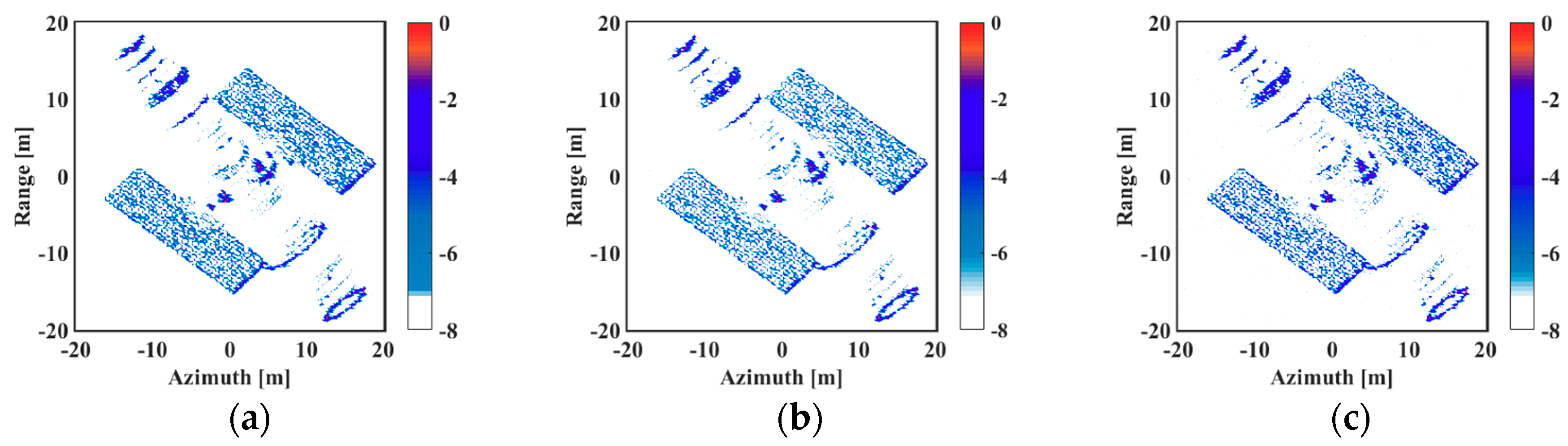
The -norm reconstruction algorithm, used in [4], and the proposed algorithm, are utilized to realize Bi-ISAR sparse imaging with RMS of 300 pulses. The magnitude of the added random phase errors are, and SNR = 10, 5, and 0 dB. The imaging results of the two algorithms are shown in Figure 10 and Figure 11, respectively. Comparing the image results in Figure 10 and Figure 11, the performance of -norm algorithm decreases more significantly as the noise increases, while the proposed algorithm can still obtain high quality images even under low SNR. The results indicate that the proposed algorithm performs better than -norm algorithm. The regularization coefficient, related to noise, influences the performance of -norm algorithm. While, the proposed method, based on full Bayesian inference, can utilize the posterior statistical information and avoid the local minimum and structural errors.
4.3. Simulations Based on an Model of Electromagnetic Scatterer
To further evaluate the proposed Bi-ISAR imaging algorithm, a simulation experiment was carried out, based on the bistatic numerical electromagnetic target data, which is the same as the data used in [21]. The satellite model is shown in Figure 12. The simulation settings in Section 4.1 are still used here.
The range profiles and the imaging results, obtained by the algorithm in [23] and the proposed algorithm in the four sparse aperture cases, are shown in Figure 13, Figure 14, Figure 15 and Figure 16, respectively. The imaging results of the two algorithms, under three different SNRs, are shown in Figure 17 and Figure 18, respectively. By comparing the imaging results, similar conclusions as found in Section 4.2 can be drawn. This is further evidence of the validity and robustness of the proposed algorithm.
5. Conclusions
For high-resolution Bi-ISAR systems with sparse aperture of space targets, we propose an imaging algorithm, which jointly realizes the MTRC correction and the sparse aperture imaging. The steps in our approach are as follows: Establishing the sparse imaging model by considering the MTRC correction and the reconstruction of the high-resolution well-focused image based on full Bayesian inference method. Simulation results, based on scatterer models of both the ideal point and the electromagnetic, confirm the effectiveness and robustness of our method.
Author Contributions
Conceptualization: L.S. and X.Z.; data curation: C.S. and J.M.; formal analysis: L.S., X.Z. and B.G.; funding acquisition: C.S., J.M. and N.H.; investigation: C.S., B.G., J.M. and N.H.; methodology: L.S., X.Z., C.S. and B.G.; validation: L.S.; writing—original draft, L.S.; writing—review and editing: X.Z., C.S. and B.G.
Funding
This research was funded by the National Natural Science Foundation of China (Grant nos. 61601496 and 61701544), the Research Innovation Development Funding of Army Engineering University Shijiazhuang Campus (Grant nos. KYSZJQZL1902), and the Natural Science Foundation of Hebei Province of China (Grant nos. F2019506031 and F2019506037).
Conflicts of Interest
The authors declare no conflicts of interest.
References
- Simon, M.P.; Schuh, M.J.; Woo, A.X. Bistatic ISAR images from a time-domain code. IEEE Antennas Propag. Mag. 1995, 37, 25–32. [Google Scholar] [CrossRef]
- Martorella, M.; Palmer, J.; Homer, J.; Littleton, B.; Longstaff, D. On bistatic inverse synthetic aperture radar. IEEE Trans. Aerosp. Electron. Syst. 2007, 43, 1125–1134. [Google Scholar] [CrossRef]
- Zhang, S.S.; Sun, S.B.; Zhang, W.; Zong, Z.L.; Yeo, T.S. High-Resolution Bistatic ISAR Image Formation for High-Speed and Complex-Motion Targets. IEEE J. Sel. Top. Appl. Earth Obs. Remote Sens. 2015, 8, 3520–3531. [Google Scholar] [CrossRef]
- Xu, G.; Xing, M.; Xia, X.; Chen, Q.; Zhang, L.; Bao, Z. High-Resolution Inverse Synthetic Aperture Radar Imaging and Scaling with Sparse Aperture. IEEE J. Sel. Top. Appl. Earth Obs. Remote Sens. 2015, 8, 4010–4027. [Google Scholar] [CrossRef]
- Xu, G.; Xing, M.; Bao, Z. High-resolution inverse synthetic aperture radar imaging of manoeuvring targets with sparse aperture. Electron. Lett. 2015, 51, 287–289. [Google Scholar] [CrossRef]
- Xu, G.; Xing, M.; Yang, L.; Bao, Z. Joint approach of translational and rotational phase error corrections for high-resolution inverse synthetic aperture radar imaging using minimum-entropy. IET Radar Sonar Navig. 2016, 10, 586–594. [Google Scholar] [CrossRef]
- Zhao, J.; Zhang, M.; Wang, X.; Cai, Z.; Nie, D. Three-dimensional super resolution ISAR imaging based on 2D unitary ESPRIT scattering centre extraction technique. IET Radar Sonar Navig. 2017, 11, 98–106. [Google Scholar] [CrossRef]
- Song, J.H.; Lee, K.W.; Lee, W.K.; Jung, C.H. High Resolution Full-Aperture ISAR Processing through Modified Doppler History Based Motion Compensation. Sensors 2017, 17, 1234. [Google Scholar] [CrossRef]
- Ma, J.T.; Gao, M.G.; Guo, B.F.; Dong, J.; Xiong, D.; Feng, Q. High resolution inverse synthetic aperture radar imaging of three-axis-stabilized space target by exploiting orbital and sparse priors. Chin. Phys. B 2017, 26, 108401. [Google Scholar] [CrossRef]
- Guo, B.F.; Wang, J.L.; Gao, M.G.; Shang, C.X.; Fu, X.J. Research on spatial-variant property of bistatic ISAR imaging plane of space target. Chin. Phys. B 2015, 24, 048402. [Google Scholar] [CrossRef]
- Ma, J.; Gao, M.; Hu, W.; Di, X.; Shi, L. Optimum Distribution of Multiple Location ISAR and Multi-angles Fusion Imaging for Space Target. J. Electron. Inf. Technol. 2017, 39, 2834–2843. [Google Scholar] [CrossRef]
- Guo, B.F.; Shang, C.X.; Wang, J.L. Bistatic ISAR echo simulation of space target based on two-body model. Syst. Eng. Electron. 2016, 38, 1771–1779. [Google Scholar] [CrossRef]
- Han, N.; Li, B.; Wang, L.; Tong, J.; Guo, B. Algorithm for autofocusing of bistatic ISAR of space target based on sparse decomposition. Acta Aeronaut. Astronaut. Sin. 2018, 39, 322037. [Google Scholar] [CrossRef]
- Shi, L.; Guo, B.F.; Ma, J.T.; Shang, C.X.; Zeng, H.Y. A Novel Channel Calibration Method for Bistatic ISAR Imaging System. Appl. Sci. 2018, 8, 2160. [Google Scholar] [CrossRef]
- Mengdao, X.; Renbiao, W.; Jinqiao, L.; Zheng, B. Migration through resolution cell compensation in ISAR imaging. IEEE Geosci. Remote Sens. Lett. 2004, 1, 141–144. [Google Scholar] [CrossRef]
- Lu, G.Y.; Bao, Z. Compensation of scatterer migration through resolution cell in inverse synthetic aperture radar imaging. IET Proc. Radar Sonar Navig. 2000, 147, 80–85. [Google Scholar] [CrossRef]
- Guo, B.F.; Shang, C.X.; Wang, J.L.; Gao, M.G.; Fu, X.J. Correction of migration through resolution cell in bistatic inverse synthetic aperture radar in the presence of time-varying bistatic angle. Acta Phys. Sin. 2014, 63, 238406. [Google Scholar]
- Muñoz-Ferreras, J.M.; Pérez-Martínez, F. Uniform rotational motion compensation for inverse synthetic aperture radar with non-cooperative targets. In IET Radar, Sonar & Navigation; Institution of Engineering and Technology: London, UK, 2008; Volume 2, pp. 25–34. [Google Scholar]
- Sun, S.B.; Jiang, Y.C.; Yuan, Y.S.; Hu, B.; Yeo, T.S. Defocusing and distortion elimination for shipborne bistatic ISAR. Remote Sens. Lett. 2016, 7, 523–532. [Google Scholar] [CrossRef]
- Tian, B.; Zou, J.; Xu, S.; Chen, Z. Squint model interferometric ISAR imaging based on respective reference range selection and squint iteration improvement. IET Radar Sonar Navig. 2015, 9, 1366–1375. [Google Scholar] [CrossRef]
- Shi, L.; Guo, B.; Han, N.; Ma, J.; Zhao, L.; Shang, C. Bistatic ISAR distortion mitigation of a space target via exploiting the orbital prior information. In IET Radar, Sonar & Navigation; Institution of Engineering and Technology: London, UK, 2019; Volume 13, pp. 1140–1148. [Google Scholar]
- Zhang, L.; Qiao, Z.; Xing, M.; Sheng, J.; Guo, R.; Bao, Z. High-Resolution ISAR Imaging by Exploiting Sparse Apertures. IEEE Trans. Antennas Propag. 2012, 60, 997–1008. [Google Scholar] [CrossRef]
- Zhu, X.X.; Hu, W.H.; Ma, J.T.; Guo, B.F.; Xue, D.F. ISAR autofocusing imaging with sparse apertures and time-varying bistatic angle. Acta Aeronaut. Astronaut. Sin. 2018, 39, 322059. [Google Scholar] [CrossRef]
- Zhang, S.; Liu, Y.; Li, X. Bayesian Bistatic ISAR Imaging for Targets with Complex Motion Under Low SNR Condition. IEEE Trans. Image Process. 2018, 27, 2447–2460. [Google Scholar] [CrossRef]
- Kang, M.; Lee, S.; Kim, K.; Bae, J. Bistatic ISAR Imaging and Scaling of Highly Maneuvering Target with Complex Motion via Compressive Sensing. IEEE Trans. Aerosp. Electron. Syst. 2018, 54, 2809–2826. [Google Scholar] [CrossRef]
- Wang, L.; Loffeld, O. ISAR imaging using a null space ℓ1 minimizing Kalman filter approach. In Proceedings of the 4th International Workshop on Compressed Sensing Theory and its Applications to Radar, Sonar and Remote Sensing (CoSeRa), Aachen, Germany, 19–22 September 2016; pp. 232–236. [Google Scholar]
- Stankovi, L.; Stankovi, I.; Dakovi, M. Analysis of noise and nonsparsity in the ISAR image recovery from a reduced set of data. In Proceedings of the 4th International Workshop on Compressed Sensing Theory and its Applications to Radar, Sonar and Remote Sensing (CoSeRa), Aachen, Germany, 19–22 September 2016; pp. 222–226. [Google Scholar]
- Baselice, F.; Ferraioli, G.; Matuozzo, G.; Pascazio, V.; Schirinzi, G. Compressive sensing for in depth focusing in 3D automotive imaging radar. In Proceedings of the 3rd International Workshop on Compressed Sensing Theory and its Applications to Radar, Sonar and Remote Sensing (CoSeRa), Pisa, Italy, 17–19 June 2015; pp. 71–74. [Google Scholar]
- Bacci, A.; Giusti, E.; Cataldo, D.; Tomei, S.; Martorella, M. ISAR resolution enhancement via compressive sensing: A comparison with state of the art SR techniques. In Proceedings of the 4th International Workshop on Compressed Sensing Theory and its Applications to Radar, Sonar and Remote Sensing (CoSeRa), Aachen, Germany, 19–22 September 2016; pp. 227–231. [Google Scholar]
- Kang, B.S.; Bae, J.H.; Kang, M.S.; Yang, E.; Kim, K.T. Bistatic-ISAR Cross-Range Scaling. IEEE Trans. Aerosp. Electron. Syst. 2017, 53, 1962–1973. [Google Scholar] [CrossRef]
- Zhu, D.; Wang, L.; Yu, Y.; Tao, Q.; Zhu, Z. Robust ISAR Range Alignment via Minimizing the Entropy of the Average Range Profile. IEEE Geosci. Remote Sens. Lett. 2009, 6, 204–208. [Google Scholar] [CrossRef]
- Wang, J.; Liu, X. Improved Global Range Alignment for ISAR. IEEE Trans. Aerosp. Electron. Syst. 2007, 43, 1070–1075. [Google Scholar] [CrossRef]
- Wei, Y.; Tat Soon, Y.; Zheng, B. Weighted least-squares estimation of phase errors for SAR/ISAR autofocus. IEEE Trans. Geosci. Remote Sens. 1999, 37, 2487–2494. [Google Scholar] [CrossRef] [Green Version]
- Morrison, R.L.; Do, M.N.; Munson, D.C. SAR Image Autofocus by Sharpness Optimization: A Theoretical Study. IEEE Trans. Image Process. 2007, 16, 2309–2321. [Google Scholar] [CrossRef]
- Wang, S.L.; Li, S.G.; Ni, J.L.; Zhang, G.Y. A New transform-match Fourier transform. Acta Electron. Sin. 2001, 29, 403–405. [Google Scholar]
Figure 1.
Geometry of bistatic ISAR imaging system.
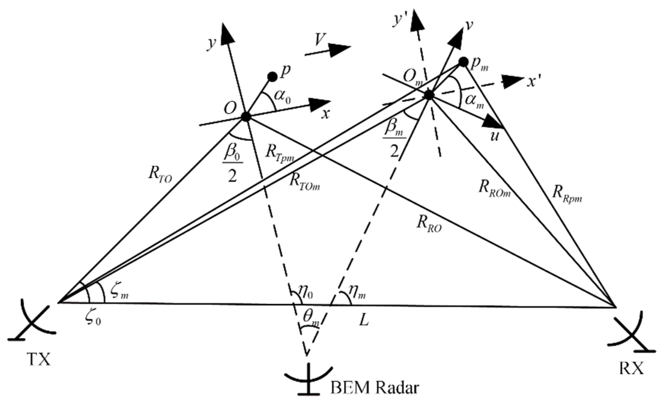
Figure 2.
Sparse aperture geometry.
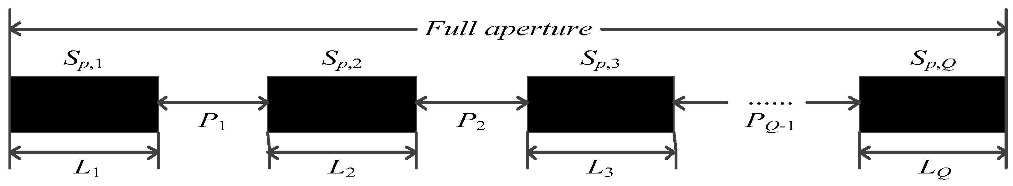
Figure 3.
Flow chart of the reconstruction algorithm.
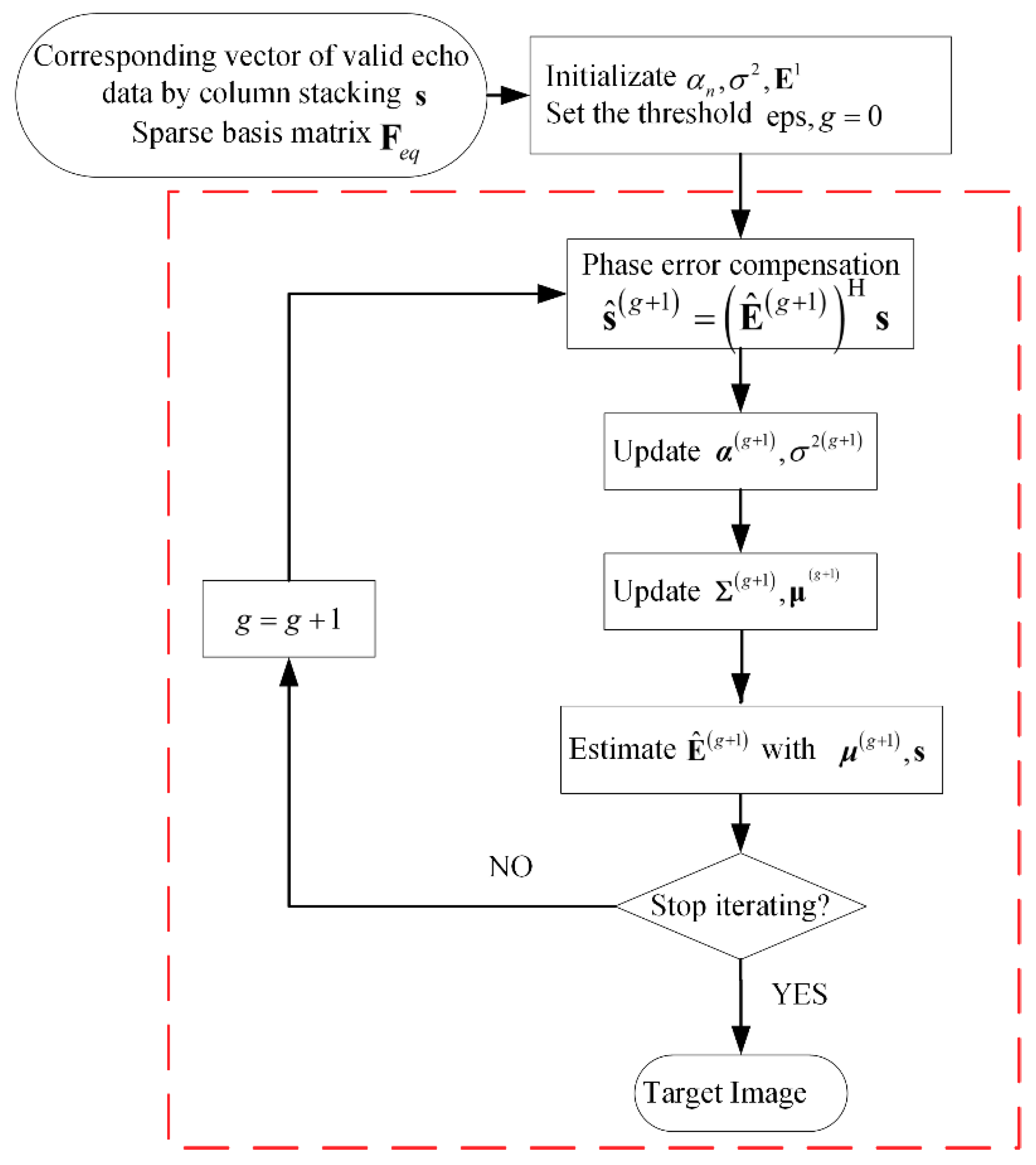
Figure 4.
Simulation scenario.
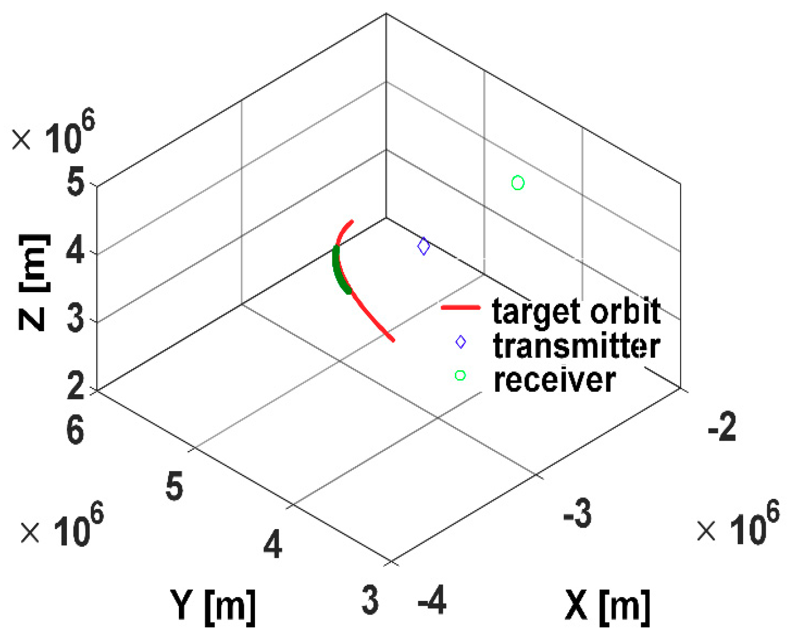
Figure 5.
The ideal point scatterer model.
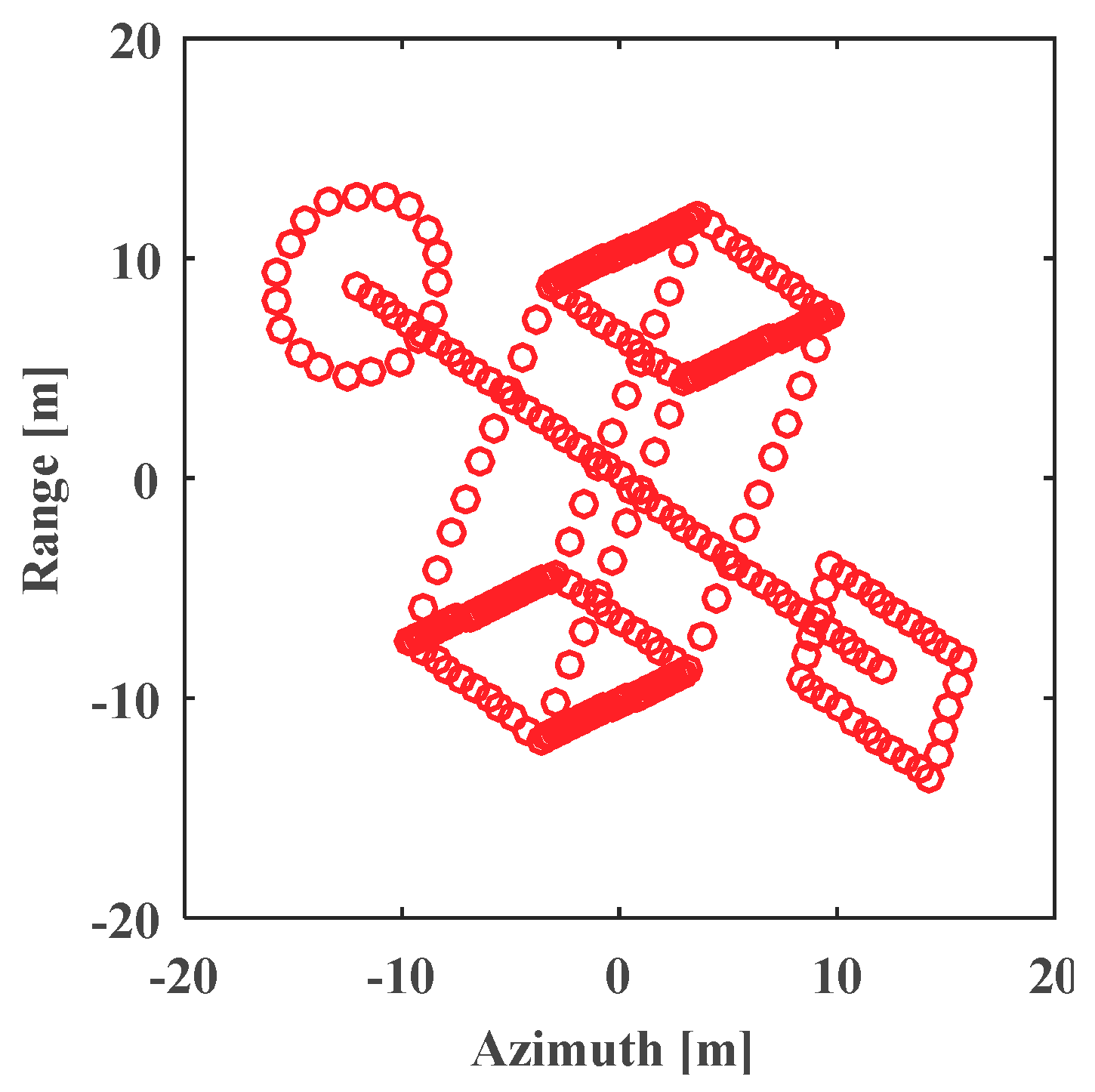
Figure 6.
Range profiles and imaging results with RMS of 300 pulses: (a) Range profiles; (b) Imaging result of algorithm in [23]; (c) Imaging result of the proposed algorithm.
Figure 6.
Range profiles and imaging results with RMS of 300 pulses: (a) Range profiles; (b) Imaging result of algorithm in [23]; (c) Imaging result of the proposed algorithm.

Figure 7.
Range profiles and imaging results with RMS of 150 pulses: (a) Range profiles; (b) Imaging result of algorithm in [23]; (c) Imaging result of the proposed algorithm.
Figure 7.
Range profiles and imaging results with RMS of 150 pulses: (a) Range profiles; (b) Imaging result of algorithm in [23]; (c) Imaging result of the proposed algorithm.
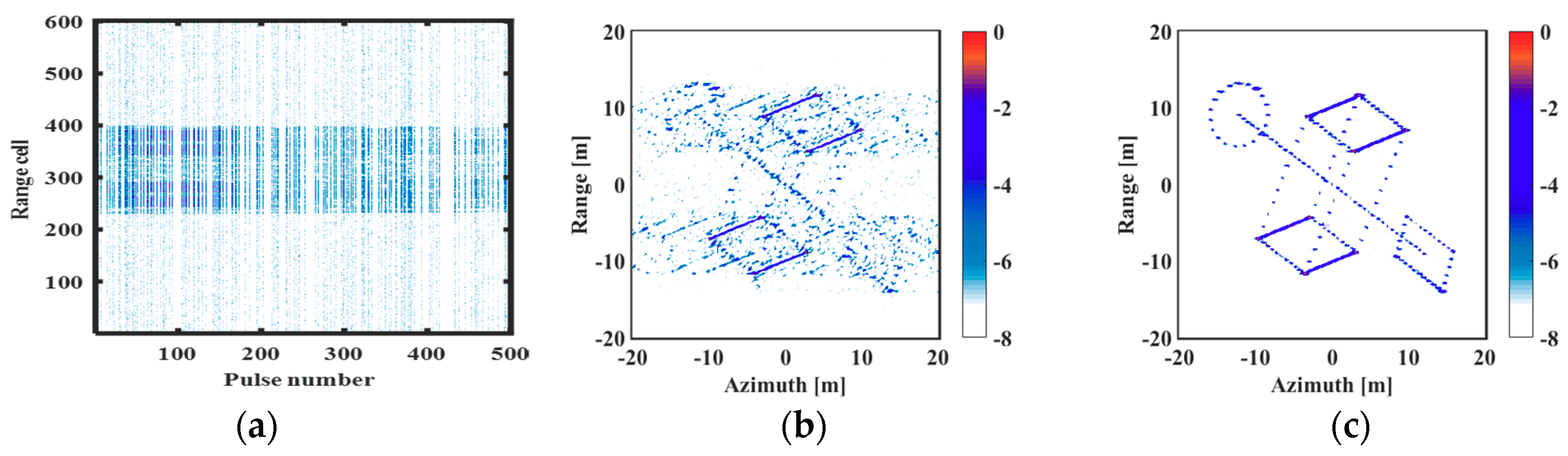
Figure 8.
Range profiles and imaging results with GMS of 300 pulses: (a) Range profiles; (b) Imaging result of algorithm in [23]; (c) Imaging result of the proposed algorithm.
Figure 8.
Range profiles and imaging results with GMS of 300 pulses: (a) Range profiles; (b) Imaging result of algorithm in [23]; (c) Imaging result of the proposed algorithm.
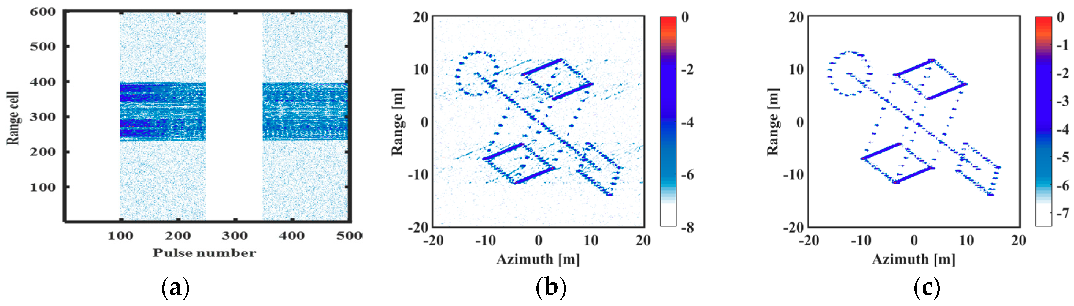
Figure 9.
Range profiles and imaging results with GMS of 150 pulses: (a) Range profiles; (b) Imaging result of algorithm in [23]; (c) Imaging result of the proposed algorithm.
Figure 9.
Range profiles and imaging results with GMS of 150 pulses: (a) Range profiles; (b) Imaging result of algorithm in [23]; (c) Imaging result of the proposed algorithm.
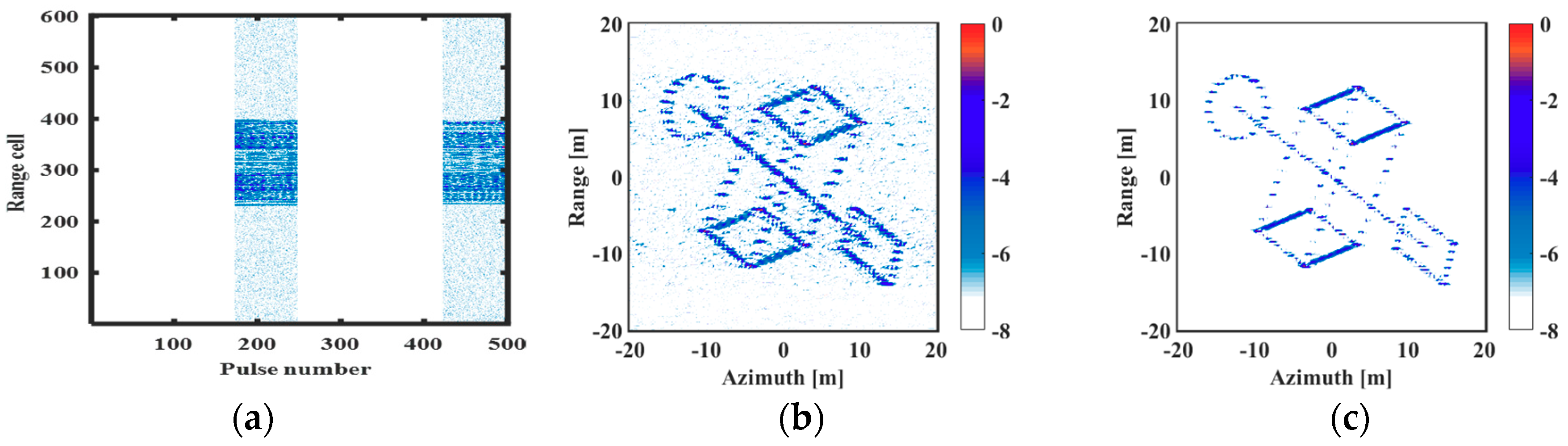
Figure 10.
Imaging results obtained by -norm algorithm under different SNRs: (a) SNR = 10 dBs; (b) SNR = 5 dB; (c) SNR = 0 dB.
Figure 10.
Imaging results obtained by -norm algorithm under different SNRs: (a) SNR = 10 dBs; (b) SNR = 5 dB; (c) SNR = 0 dB.
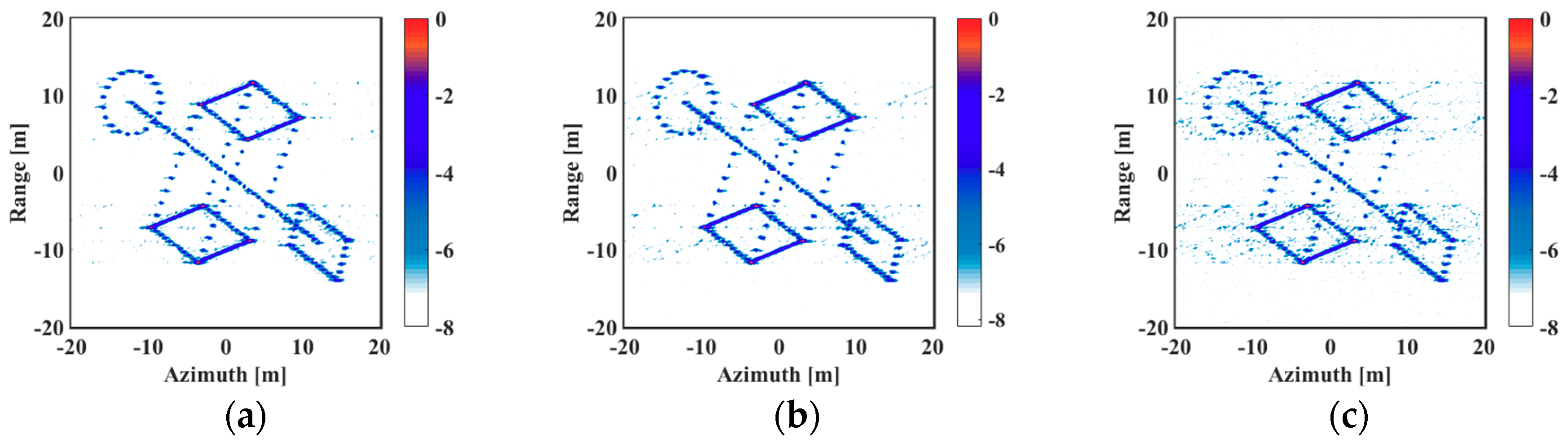
Figure 11.
Imaging results obtained by the proposed algorithm under different SNRs: (a) SNR = 10 dB; (b) SNR = 5 dB; (c) SNR = 0 dB.
Figure 11.
Imaging results obtained by the proposed algorithm under different SNRs: (a) SNR = 10 dB; (b) SNR = 5 dB; (c) SNR = 0 dB.
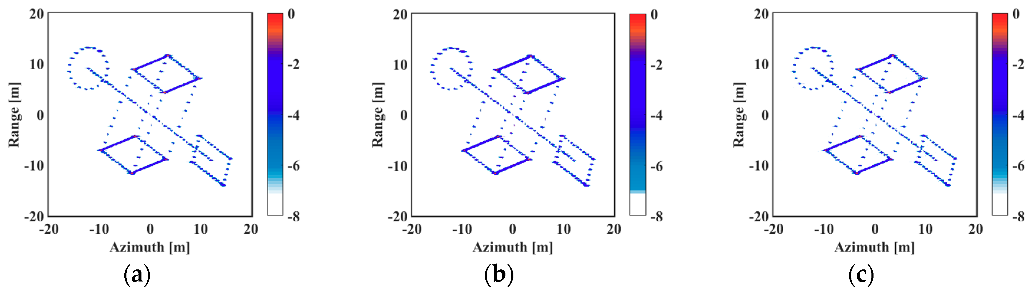
Figure 12.
The side view of the model of typical satellite (40.09 m × 30.37 m × 20.74 m).
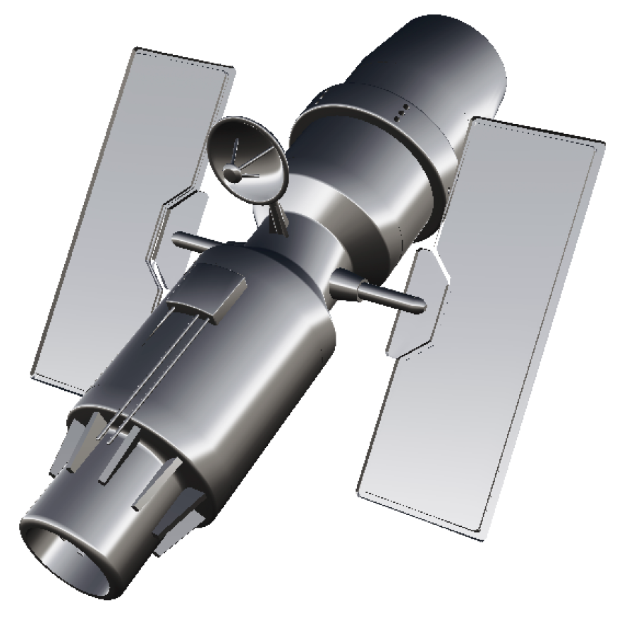
Figure 13.
Range profiles and imaging results with RMS of 300 pulses: (a) Range profiles; (b) Imaging result of algorithm in [23]; (c) Imaging result of the proposed algorithm.
Figure 13.
Range profiles and imaging results with RMS of 300 pulses: (a) Range profiles; (b) Imaging result of algorithm in [23]; (c) Imaging result of the proposed algorithm.
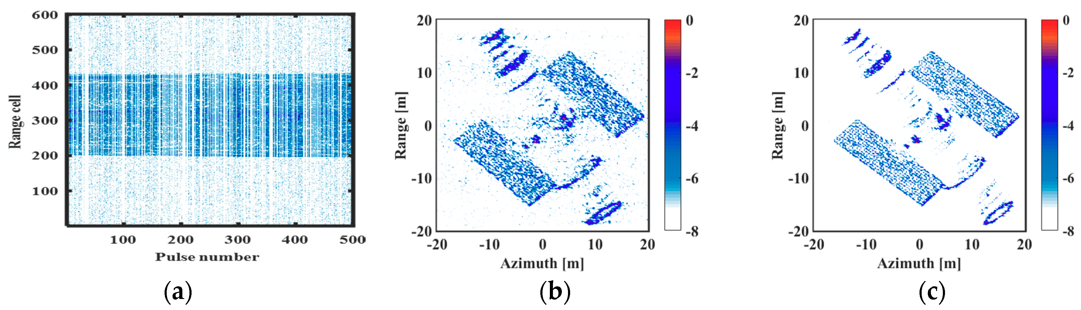
Figure 14.
Range profiles and imaging results with RMS of 150 pulses: (a) Range profiles; (b) Imaging result of algorithm in [23]; (c) Imaging result of the proposed algorithm.
Figure 14.
Range profiles and imaging results with RMS of 150 pulses: (a) Range profiles; (b) Imaging result of algorithm in [23]; (c) Imaging result of the proposed algorithm.
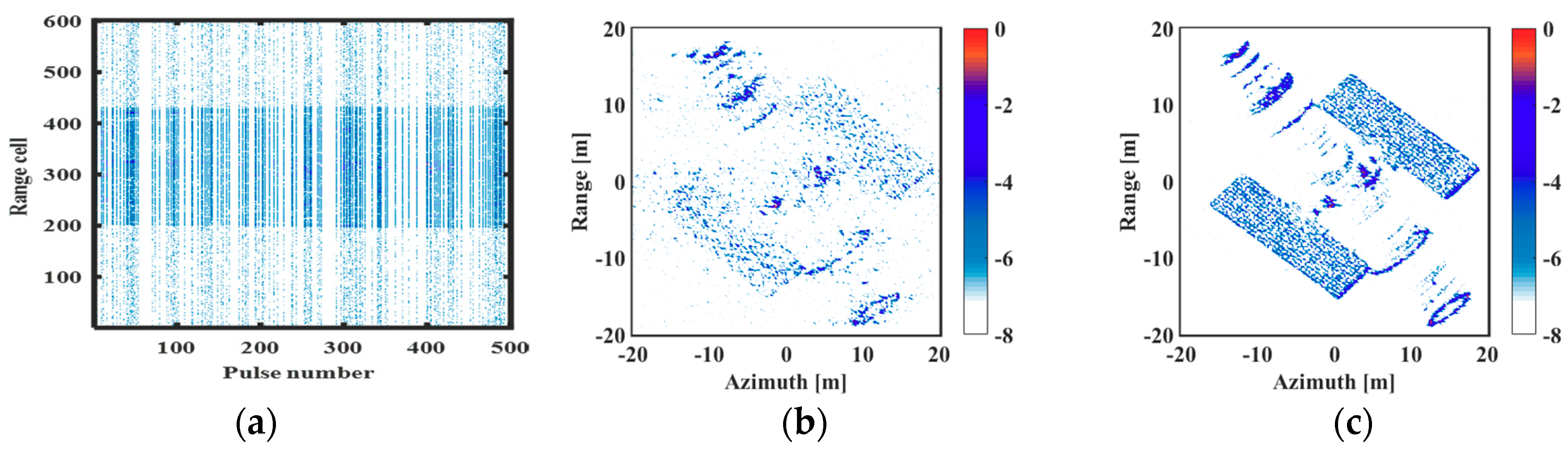
Figure 15.
Range profiles and imaging results with GMS of 300 pulses: (a) Range profiles; (b) Imaging result of algorithm in [23]; (c) Imaging result of the proposed algorithm.
Figure 15.
Range profiles and imaging results with GMS of 300 pulses: (a) Range profiles; (b) Imaging result of algorithm in [23]; (c) Imaging result of the proposed algorithm.
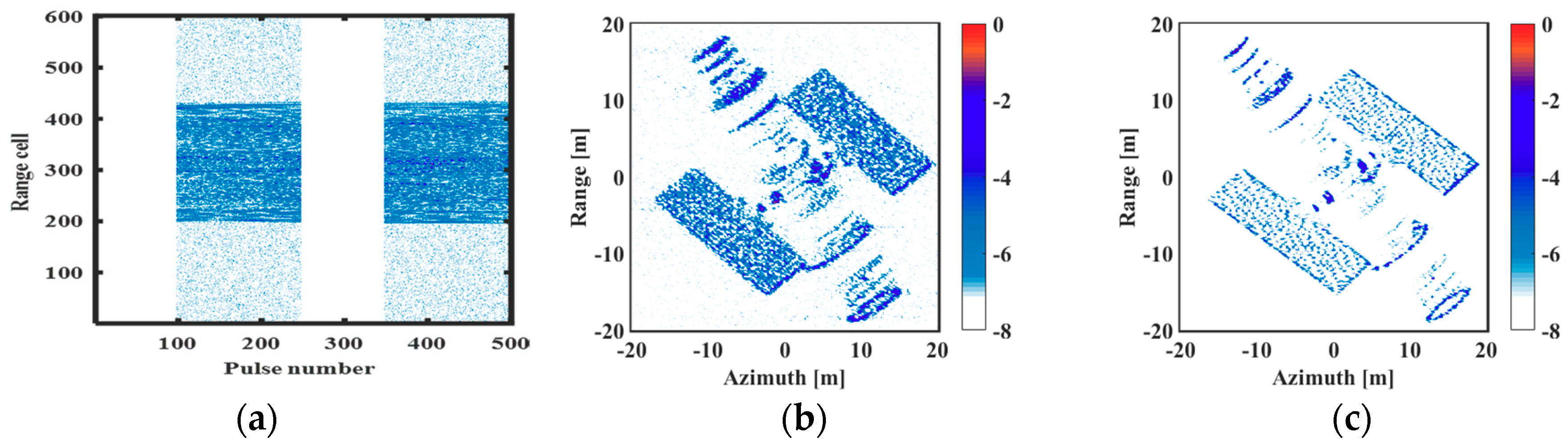
Figure 16.
Range profiles and imaging results with GMS of 150 pulses: (a) Range profiles; (b) Imaging result of algorithm in [23]; (c) Imaging result of the proposed algorithm.
Figure 16.
Range profiles and imaging results with GMS of 150 pulses: (a) Range profiles; (b) Imaging result of algorithm in [23]; (c) Imaging result of the proposed algorithm.
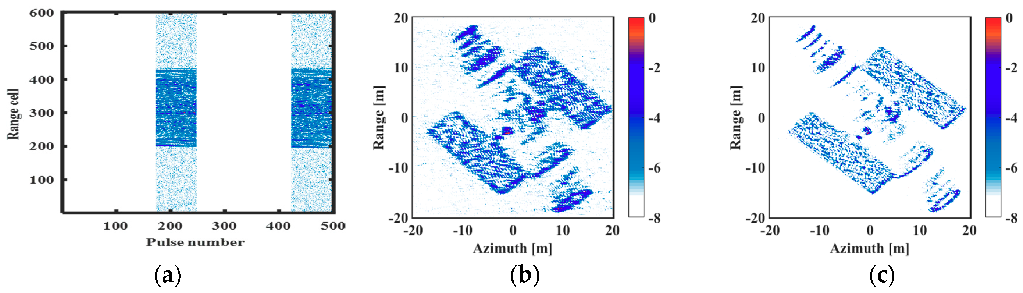
Figure 17.
Imaging results obtained by -norm algorithm under different SNRs: (a) SNR = 10 dBs; (b) SNR = 5 dB; (c) SNR = 0 dB.
Figure 17.
Imaging results obtained by -norm algorithm under different SNRs: (a) SNR = 10 dBs; (b) SNR = 5 dB; (c) SNR = 0 dB.

Figure 18.
Imaging results obtained by the proposed algorithm under different SNRs: (a) SNR = 10 dB; (b) SNR = 5 dB; (c) SNR = 0 dB.
Figure 18.
Imaging results obtained by the proposed algorithm under different SNRs: (a) SNR = 10 dB; (b) SNR = 5 dB; (c) SNR = 0 dB.

Table 1.
Parameters of the Simulation.
| Parameter Name | Value | Parameter Name | Value |
|---|---|---|---|
| Carrier frequency | 10 GHz | Signal bandwidth | 1000 MHz |
| Pulse width | 20 us | Sampling frequency | 1200 MHz |
| Pulse Repetition Frequency | 50 Hz | Accumulation numbers | 500 |
| Chirp rate | 5 × 10¹³ | Equivalent Doppler bandwidth | 10 s |
| Range resolution | 0.1809 m | Azimuth resolution | 0.2683 m |
© 2019 by the authors. Licensee MDPI, Basel, Switzerland. This article is an open access article distributed under the terms and conditions of the Creative Commons Attribution (CC BY) license (http://creativecommons.org/licenses/by/4.0/).
Share and Cite
MDPI and ACS Style
Shi, L.; Zhu, X.; Shang, C.; Guo, B.; Ma, J.; Han, N. High-Resolution Bistatic ISAR Imaging of a Space Target with Sparse Aperture. Electronics 2019, 8, 874. https://doi.org/10.3390/electronics8080874
AMA Style
Shi L, Zhu X, Shang C, Guo B, Ma J, Han N. High-Resolution Bistatic ISAR Imaging of a Space Target with Sparse Aperture. Electronics. 2019; 8(8):874. https://doi.org/10.3390/electronics8080874
Chicago/Turabian StyleShi, Lin, Xiaoxiu Zhu, Chaoxuan Shang, Baofeng Guo, Juntao Ma, and Ning Han. 2019. "High-Resolution Bistatic ISAR Imaging of a Space Target with Sparse Aperture" Electronics 8, no. 8: 874. https://doi.org/10.3390/electronics8080874
Note that from the first issue of 2016, this journal uses article numbers instead of page numbers. See further details here.