Visual Closed-Loop Dynamic Model Identification of Parallel Robots Based on Optical CMM Sensor

Abstract

Parallel robots present outstanding advantages compared with their serial counterparts; they have both a higher force-to-weight ratio and better stiffness. However, the existence of closed-chain mechanism yields difficulties in designing control system for practical applications, due to its highly coupled dynamics. This paper focuses on the dynamic model identification of the 6-DOF parallel robots for advanced model-based visual servoing control design purposes. A visual closed-loop output-error identification method based on an optical coordinate-measuring-machine (CMM) sensor for parallel robots is proposed. The main advantage, compared with the conventional identification method, is that the joint torque measurement and the exact knowledge of the built-in robot controllers are not needed. The time-consuming forward kinematics calculation, which is employed in the conventional identification method of the parallel robot, can be avoided due to the adoption of optical CMM sensor for real time pose estimation. A case study on a 6-DOF RSS parallel robot is carried out in this paper. The dynamic model of the parallel robot is derived based on the virtual work principle, and the built dynamic model is verified through Matlab/SimMechanics. By using an outer loop visual servoing controller to stabilize both the parallel robot and the simulated model, a visual closed-loop output-error identification method is proposed and the model parameters are identified by using a nonlinear optimization technique. The effectiveness of the proposed identification algorithm is validated by experimental tests.

1. Introduction

Parallel robots are closed-chain mechanisms in which the end-effector is supported by a series of independent computer-controlled serial chains linked to the base platform. Parallel robots present some outstanding advantages in higher force-to-weight ratio and better stiffness compared with serial manipulators. Specifically, 6-DOF parallel robots have been used in various applications (e.g., flight simulators [1], manufacturing lines [2] and medical tools [3]). Due to the manufacturing tolerances and deflection in the robot structure, the typical positioning discrepancy between a virtual robot in simulation and a real robot can be 8–15 mm [4], which does not meet the precision requirement of many potential applications. The low absolute accuracy of the robot is the main problem for the off-line programming based applications where tens of thousand points or continuous trajectories are to be reached or tracked.

The existence of closed-chain mechanism and multiple moving parts in the parallel robots, for example, in a 6-DOF Gough-Stewart platform consisting of 13 moving bodies (12 legs and one end-effector), yields difficulties in dynamic analysis of parallel robots. Moreover, the dynamic model plays an important role in the model-based controller designs, especially in applications where high positioning and tracking accuracy is needed. In contrast to serial robots, where the joint angles are used as the state variables for modeling, the parallel robots are preferably modeled and controlled in the operational (workspace) coordinates where the pose of the end-effector and its derivatives are used as the state variables [5]. The main reason is that there is almost no analytical expression for the forward kinematic model of 6-DOF parallel robots. For example, there are 40 forward kinematics solutions [6] mapping the joint coordinates to the pose of the end-effector platform in a Gough-Stewart platform. In addition, to this day, there is no effective method to determine the pose of the platform from multiple solutions. The dynamic models of 6-DOF Gough-Stewart parallel robot have been built by several approaches such as Newton-Euler [7], Lagrangian formulation [8] and the principle of virtual work [9]. Newton-Euler formulation can provide the internal forces for each individual body of the parallel robot, which can benefit the mechanical design process of the parallel robot. However, the computational load is high due to the large amount of equations. In contrast, the Lagrangian and virtual work methods are more efficient and suitable for the control design purpose since the reaction forces between the bodies of the parallel robot are not considered. The published research work on 6-DOF RSS parallel robots is considerably scarcer compared with that on Gough-Stewart parallel robot. The dynamic models of one type of 6-DOF RSS parallel robot, in which the active rotation axes are coplanar, are built based on Newton-Euler equations [10] or Lagrangian formulation [11] for dynamic analysis and tracking control purpose respectively. In this paper, the dynamic model of a 6-DOF RSS parallel robot, where the active rotation axes are parallel to each other, is built based on the virtual work principle, and the explicit form of the dynamic model is derived for identification and dynamic model-based visual servoing purposes.

The dynamic parameters are normally unknown or approximately derived from manufacturer specifications, which are not accurate enough for the dynamic model-based controller design. System identification is an effective method to perceive the uncertain parameters in the dynamic model of the system, and has been applied to many engineering practices [12]. As a highly coupled multi-input/multi-output (MIMO) nonlinear system, industrial robots aroused great interest and challenge for the identification method. The literatures on the state-of-the-art identification methods can be found in [13,14,15]. For the industrial robots, the dynamic identification is normally performed in closed-loop, since the robotic system is open loop unstable. In [16], a MIMO closed-loop identification based on weighted least square estimation has been applied to an industrial serial robot used in a planar configuration. In addition, other closed-loop identification methods with maximum likelihood, instrumental variable and related implementation issues on industrial serial robots are addressed in [17,18]. A new closed-loop output-error identification scheme has been adopted for the serial robots [19]. The output-error identification method aims at finding the dynamic model parameters by minimizing the output deviation between the actual and simulated systems subjecting to the same input [20]. In [19], the identification procedure is implemented in a closed-loop control structure and the joint torque is the measured output, which avoids the estimation of the velocity and acceleration from the measured joint position.

One potential issue of the above-mentioned identification methods is that joint torque measurement or a related control signal is needed for identification, which is not always available for the industrial robots, since the built-in controllers of many industrial robots are unaccessible and do not provide the torque actuation mode [21]. The input of built-in controllers is the position or velocity command, and the output is the joint torque which is unaccessible to the users. Hence the torque and current of the motors cannot be derived directly and it is not easy to install additional torque sensors to get the direct measurement. The unknown controller can be identified along with the dynamic parameters as introduced in [22]. However, joint torque measurement is still needed for identification purposes.

In [13,23,24,25], identification issues in parallel robots have been discussed. Most research works on dynamic identification of parallel robots are based on a simplified dynamic model, such as in [26,27,28]. Nevertheless, the systematic derivation of the full inverse dynamic model is proposed based on Jourdain’s principle in [24]. In addition, the identification procedure is carried out in two steps: 1. identifying inertial parameters and 2. estimating the friction coefficients. In [23], the full parameters of robots’ dynamic model and the joint drive gains are identified based on the total least square method, and the method is tested on a 3 DOF Orthoglide parallel robot. Many identification methods for 6 DOF parallel robots in [23,24,25] come directly from those of serial robots. By rewriting the inverse dynamic model and friction model into a linear form with respect to the dynamic and friction parameters, the identification of the unknown parameters can be done through least squares technique. However for 6 DOF parallel robots, to avoid solving forward kinematics, the regression matrix of the dynamic model is constituted of the pose state variables in the operational space. In [25], only joint space state variables are measured and estimated. Therefore the state variables in operational space should be calculated through numerical computation of the forward kinematics, which is quite time-consuming.

One way to avoid computing the forward kinematics in the identification process is to directly measure the pose of the end-effector in the operational space based on vision sensors. In [28], a camera-based dynamic identification procedure is given for a 4-DOF parallel robot with a heavily simplified dynamic model by considering only the inertia of the end-effector. Also, a vision sensor based dynamic identification has been carried out on serial robots [29] and cable robots [30], but seldom on parallel robots. The optical CMM sensor is a dual camera based vision sensor, which can provide the real-time pose information of the targets. The coordinates of target reflectors in the field of view (FOV) can be directly measured by the sensor. By observing four non-collinear reflectors on the platform, the pose of the end-effector can be measured. The optical CMM sensor has been applied to the kinematics calibration [31] and the path tracking controller design [32] for the robots. To increase the flexibility and tracking accuracy, vision can also be incorporated into the feedback control loop of the parallel robot systems to form the so-called visual servoing control. The pose of the end-effector can be acquired on-line by using the optical CMM sensor, i.e., C-track from Creaform Inc. (Levis, QC, Canada). The visual servoing controller for parallel robot is superior to the joint space controller due to the fact that the kinematic errors introduced from transforming the desired trajectory in the operational space into the one in the joint space in the joint controller can be avoided. The measured pose together with the visual servoing controller allows using the closed-loop output-error identification method [20] to identify the dynamic model of the parallel robot.

Upon the above discussions, a closed-loop output-error identification method based on a CMM sensor is proposed for parallel robots in this paper. The end-effector pose is measured by the optical CMM and served as the output of the real plant. The same outer loop visual servoing controller and reference trajectory are employed in both actual robot and simulation model for model identification. The forward kinematics of parallel robots, which is usually solved by using time-consuming numerical algorithm, can be avoided. The exact knowledge of the built-in controller and the joint torque are not needed. The dynamic model parameters are identified by using nonlinear optimization technique. The experimental tests validate the identification results.

This paper is organized as follows. Section 2 describes the dynamic model of a 6-RSS parallel robot. The closed-loop output-error identification method is proposed and the procedure of the identification is presented in Section 3. The dynamic model validation based on simulation and the experiment results of the identification are given in Section 4. Finally, the conclusion is drawn in Section 5.

2. Dynamic Modeling

In this section, the kinematic analysis of a 6 RSS parallel robot is conducted and the dynamic model is derived based on the virtual work principle.

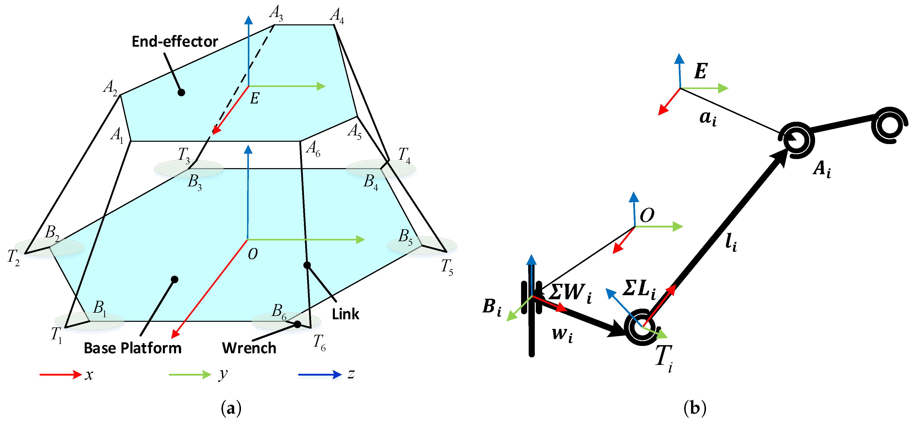
2.1. Kinematic Analysis

The motivation of kinematic analysis is to determine geometry mapping from the motion of end-effector frame w.r.t the base frame (operational space motion) to the rotation of the actuators, as regarding the revolute joint frames (joint space motion). Based on the geometry mapping, the link Jacobian matrix is derived for building the dynamic model. As shown in Figure 1a, the 6-RSS parallel robot consists of six identical serial branch chains. Each serial branch, illustrated in Figure 1b, consists of a wrench, a link, an active revolute joint (R) and two passive spherical joints (S). One spherical joint is used to connect the wrench and the link. The revolute joint is driven by actuators and connects the wrench and the base platform, while the spherical joint is employed between the link and the end effector. The base frame $\Sigma O$ is assigned at the symmetric center of the base platform and the end-effector frame $\Sigma E$ is also attached at the symmetric center, while $\mathit{E}$ denotes the coordinate vector of the frame origin regarding the base frame. The coordinate vectors of revolute joint centers regarding the base frame are marked by ${\mathit{B}}_{\mathit{i}}(i=1,2,\dots ,6)$ while the rotation centers of spherical joints are represented as ${\mathit{T}}_{\mathit{i}}$ and ${\mathit{A}}_{\mathit{i}}$ respectively. In the subsequent kinematic and dynamic analysis, the coordinates of the parts of parallel robot are defined regarding the base frame by default. The moving wrench and link frames $\Sigma W_i$ and $\Sigma L_i$ are attached to the wrenches and links respectively as depicted in Figure 1b. The coordinate vectors of the centers of mass of the wrenches and links are denoted as ${\mathit{c}}_{{\mathit{w}}_{\mathit{i}}}$ and ${\mathit{c}}_{{\mathit{l}}_{\mathit{i}}}$ respectively. The vector $\mathit{\theta }={[{\theta }_1,{\theta }_2,\dots ,{\theta }_6]}^T$ represents the rotation angles of the actuators. The coordinate vector from $\mathit{E}$ pointing to ${\mathit{A}}_{\mathit{i}}$ regarding the end-effector frame is denoted as ${\mathit{a}}_{\mathit{i}}$. And the coordinate vectors ${\mathit{w}}_{\mathit{i}}$ and ${\mathit{l}}_{\mathit{i}}$ represent the directions and length of the wrench and link. The pose vector of the end-effector frame is expressed as ${\mathit{\chi }}_{\mathit{E}}={\left[\mathit{h},\mathit{\varphi }\right]}^T$, where $\mathit{h}={[x,y,z]}^T$ represents the position of the end-effector frame origin, while $\mathit{\varphi }={[\alpha ,\beta ,\gamma ]}^T$ represents the Euler-angle rotation of the frame. The rotation matrix, R, is given by

$$R=R_x\left(\alpha \right)R_y\left(\beta \right)R_z\left(\gamma \right)=\left(\begin{array}{ccc}c\beta c\gamma & -c\beta s\gamma & s\beta \\ c\alpha s\gamma +c\gamma s\beta s\alpha & -s\beta s\alpha s\gamma +c\alpha c\gamma & -c\beta s\alpha \\ s\alpha s\gamma -c\alpha c\gamma s\beta & c\alpha s\beta s\gamma +c\gamma s\alpha & c\beta c\alpha \end{array}\right),$$

(1)

where $R_x,R_y,R_z$ are the orthonormal rotation matrices for the rotation about $X,Y,Z$ axes respectively. The vector ${\dot{\mathit{\chi }}}_{\mathit{E}}={\left[{\dot{\mathit{h}}}^T,{\dot{\mathit{\varphi }}}^T\right]}^T$ and ${\ddot{\mathit{\chi }}}_{\mathit{E}}={\left[{\ddot{\mathit{h}}}^T,{\ddot{\mathit{\varphi }}}^T\right]}^T$ are the first and second order time derivatives of ${\mathit{\chi }}_{\mathit{E}}$. The vector ${\mathit{v}}_{\mathit{E}}={\left[{\dot{\mathit{h}}}^T,{\mathit{\omega }}^T\right]}^T\in R^{6\times 1}$ denotes the linear and angular velocities of the end-effector frame. Then ${\dot{\mathit{v}}}_{\mathit{E}}$ is the acceleration vector. The relationship between the Euler angle rate $\dot{\mathit{\varphi }}$ and angular velocity $\mathit{\omega }$ is expressed as follows

$$\mathit{\omega }=J_e\dot{\mathit{\varphi }},$$

(2)

where $J_e=\left[\begin{array}{ccc}1& 0& s\beta \\ 0& c\alpha & -c\beta s\alpha \\ 0& s\alpha & c\beta c\alpha \end{array}\right]$ is the analytical Jacobian matrix, s and c stand for $sin$ and $cos$ respectively.

The following assumptions are made for kinematic and dynamic analysis of a 6-RSS parallel robot:

• The end-effector platform, wrenches and links are symmetric with respect to their axes.
• The links do not rotate about its symmetric axes.

As shown in Figure 1a,b, the closure loop position relationship between the end-effector frame and the base frame can be expressed as the following:

$$\mathit{E}+{\mathit{a}}_{\mathit{i}}-{\mathit{A}}_{\mathit{i}}=0and$$

(3)

$${\mathit{B}}_{\mathit{i}}+{\mathit{w}}_{\mathit{i}}+{\mathit{l}}_{\mathit{i}}-{\mathit{A}}_{\mathit{i}}=0,i=1,2,\dots ,6.$$

(4)

Then the linear velocity can be derived by combining Equations (3) and (4) and taking the time derivative:

$$\dot{\mathit{h}}+\mathit{\omega }\times {\mathit{a}}_{\mathit{i}}={\mathit{\omega }}_{\mathbf{1}}\times {\mathit{w}}_{\mathit{i}}+{\mathit{\omega }}_{\mathbf{2}}\times {\mathit{l}}_{\mathit{i}},i=1,2,\dots ,6,$$

(5)

where ${\mathit{\omega }}_{\mathbf{1}}$ and ${\mathit{\omega }}_{\mathbf{2}}$ are the angular velocity of frame $\Sigma W_i$ and $\Sigma L_i$ regarding $\Sigma O$ respectively.

Then, dot multiplying ${\mathit{l}}_{\mathit{i}}$ on both sides of Equation (5) yields:

$$\begin{array}{c}\hfill {\mathit{l}}_{\mathit{i}}\dot{\mathit{h}}+({\mathit{a}}_{\mathit{i}}\times {\mathit{l}}_{\mathit{i}})\mathit{\omega }=({\mathit{w}}_{\mathit{i}}\times {\mathit{l}}_{\mathit{i}})·{\mathit{\omega }}_{\mathbf{1}},i=1,2,\dots ,6.\end{array}$$

(6)

Since the wrench rotates around a fixed axis which is denoted as $\widehat{\mathit{s}}={[0,0,1]}^T$, the Jacobian matrix mapping from the end-effector Cartesian velocity to joint velocity can be derived by the following:

$$J_{a1}\dot{\mathit{\theta }}=J_{a2}{\mathit{v}}_{\mathit{E}},$$

(7)

where $J_{a1}=diag(({\mathit{w}}_{\mathbf{1}}\times {\mathit{l}}_{\mathbf{1}})·\widehat{\mathit{s}},({\mathit{w}}_{\mathbf{2}}\times {\mathit{l}}_{\mathbf{2}})·\widehat{\mathit{s}},\dots ,({\mathit{w}}_{\mathbf{6}}\times {\mathit{l}}_{\mathbf{6}})·\widehat{\mathit{s}})$, $J_{a2}=\left[\begin{array}{cc}{{\mathit{l}}_{\mathbf{1}}}^T& {({\mathit{a}}_{\mathbf{1}}\times {\mathit{l}}_{\mathbf{1}})}^T\\ ⋮& ⋮\\ {{\mathit{l}}_{\mathbf{6}}}^T& {({\mathit{a}}_{\mathbf{6}}\times {\mathit{l}}_{\mathbf{6}})}^T\end{array}\right]$.

When the robot works in the singularity-free operational space, the Jacobian matrix $J_{ad}$ can be derived as follows:

$$\dot{\mathit{\theta }}=J_{a1}^{-1}{J}_{a2}{\mathit{v}}_{\mathit{E}}=J_{ad}{\mathit{v}}_{\mathit{E}}.$$

(8)

Then the translational velocity of the center of mass of the wrench $\dot{{\mathit{c}}_{{\mathit{w}}_{\mathit{i}}}}$ can be obtained from Equation (9).

$$\dot{{\mathit{c}}_{{\mathit{w}}_{\mathit{i}}}}={\dot{\theta }}_i\widehat{\mathit{s}}\times {\mathit{c}}_{{\mathit{w}}_{\mathit{i}}}=J_{au}{\mathit{v}}_{\mathit{E}},$$

(9)

where $J_{au}=(\widehat{\mathit{s}}\times {\mathit{c}}_{{\mathit{w}}_{\mathit{i}}})J_{adi}\in R^{3\times 6}$, and $J_{adi}$ is the ith row of $J_{ad}$. Then the link Jacobian $J_a$ mapping ${\mathit{v}}_{\mathit{E}}$ to the velocity of the center of mass of the ith wrench ${\mathit{v}}_{\mathbf{1}}={[{\dot{{\mathit{c}}_{{\mathit{w}}_{\mathit{i}}}}}^T,{\mathit{\omega }}_{1i}^T]}^T$ can be derived as

$${\mathit{v}}_{\mathbf{1}}=\left[\begin{array}{c}\dot{{\mathit{c}}_{w_i}}\\ {\mathit{\omega }}_{\mathbf{1}\mathit{i}}\end{array}\right]=\left[\begin{array}{c}{J}_{au}\\ \widehat{\mathit{s}}{J}_{adi}\end{array}\right]{\mathit{v}}_{\mathit{E}}=J_a{\mathit{v}}_{\mathit{E}}.$$

(10)

Equation (11) can be deduced by right cross multiplying ${\mathit{l}}_{\mathit{i}}$ on the both sides of Equation (5) and using Lagrange’s rule.

$$\begin{array}{c}\hfill ({\mathit{\omega }}_{\mathbf{2}}·{\mathit{l}}_{\mathit{i}})·{\mathit{l}}_{\mathit{i}}-({\mathit{l}}_{\mathit{i}}·{\mathit{l}}_{\mathit{i}})·{\mathit{\omega }}_{\mathbf{2}}=\dot{\mathit{h}}\times {\mathit{l}}_{\mathit{i}}+(\mathit{\omega }\times {\mathit{a}}_{\mathit{i}})\times {\mathit{l}}_{\mathit{i}}-({\mathit{\omega }}_{\mathbf{1}}\times {\mathit{w}}_{\mathit{i}})\times {\mathit{l}}_{\mathit{i}}.\end{array}$$

(11)

Since the link does not rotate about its longitudinal axis, ${\mathit{\omega }}_{\mathbf{2}}·{\mathit{l}}_{\mathit{i}}=0$ holds. Rearranging Equation (11), the following equation can be derived:

$$\begin{array}{c}\Vert {\mathit{l}}_{\mathit{i}}{\Vert }^2{\mathit{\omega }}_{\mathbf{2}}={\left[{\mathit{l}}_{\mathit{i}}\right]}_X\dot{\mathit{h}}-{\left[{\mathit{l}}_{\mathit{i}}\right]}_X{\left[{\mathit{a}}_{\mathit{i}}\right]}_X\mathit{\omega }+{\left[{\mathit{l}}_{\mathit{i}}\right]}_X{\left[{\mathit{w}}_{\mathit{i}}\right]}_X{\mathit{\omega }}_{\mathbf{1}},\hfill \end{array}$$

(12)

where the operator ${[·]}_X$ and $\Vert ·\Vert$ represents the cross product operation and Euclidean norm respectively.

By combining Equations (8) and (12), the following Jacobian matrix $J_{bd}$ mapping from the end-effector Cartesian velocity to the angular velocity of the link frame can be deduced:

$$\begin{array}{c}{\mathit{\omega }}_{\mathbf{2}}=J_{bd}{\mathit{v}}_{\mathit{E}},\\ J_{bd}=\frac{1}{\Vert {\mathit{l}}_{\mathit{i}}{\Vert }^2}\{\left[\begin{array}{c}{\left[{\mathit{l}}_{\mathit{i}}\right]}_X-{\left[{\mathit{l}}_{\mathit{i}}\right]}_X{\left[{\mathit{a}}_{\mathit{i}}\right]}_X\end{array}\right]+{\left[{\mathit{l}}_{\mathit{i}}\right]}_X{\left[{\mathit{w}}_{\mathit{i}}\right]}_X\widehat{\mathit{s}}{J}_{adi}\}.\end{array}$$

(13)

The translational velocity of the center of mass of the link $\dot{{\mathit{c}}_{{\mathit{l}}_{\mathit{i}}}}$ can be obtained as follows:

$$\dot{{\mathit{c}}_{{\mathit{l}}_{\mathit{i}}}}=-{\left[{\mathit{w}}_{\mathit{i}}\right]}_X{\mathit{\omega }}_{\mathbf{1}}-{\left[{\mathit{c}}_{{\mathit{l}}_{\mathit{i}}}\right]}_X{\mathit{\omega }}_{\mathbf{2}}$$

(14)

By substituting Equations (10) and (13) into Equation (14), the following velocity relationship can be derived:

$$\dot{{\mathit{c}}_{{\mathit{l}}_{\mathit{i}}}}=(-{\left[{\mathit{w}}_{\mathit{i}}\right]}_X\widehat{\mathit{s}}{J}_{adi}-{\left[{\mathit{c}}_{{\mathit{l}}_{\mathit{i}}}\right]}_X{J}_{bd}){\mathit{v}}_{\mathit{E}}=J_{bu}{\mathit{v}}_{\mathit{E}}$$

(15)

Hence the link Jacobian $J_b$ mapping ${\mathit{v}}_{\mathit{E}}$ to the velocity of the center of mass of the ith link ${\mathit{v}}_{\mathbf{2}}$ can be derived.

$${\mathit{v}}_{\mathbf{2}}=\left[\begin{array}{c}\dot{{\mathit{c}}_{{\mathit{l}}_{\mathit{i}}}}\\ {\mathit{\omega }}_{\mathbf{2}\mathit{i}}\end{array}\right]=\left[\begin{array}{c}{J}_{bu}\\ J_{bd}\end{array}\right]{\mathit{v}}_{\mathit{E}}=J_b{\mathit{v}}_{\mathit{E}}$$

(16)

2.2. Dynamic Modeling

In contrast to serial robots, the dynamic modeling of parallel robots is more complicated due to its closure geometrical structure and difficulties in deriving the forward kinematics. The principle of virtual work is employed to derive the explicit form of the dynamic model in terms of the operational coordinates and their time derivatives as shown in Equation (17) for 6-DOF RSS robot, which is useful for dynamic model-based controller design.

$${\mathit{\tau }}_{\mathit{g}}=M\left({\mathit{\chi }}_{\mathit{E}}\right){\dot{\mathit{v}}}_{\mathit{E}}+C({\mathit{\chi }}_{\mathit{E}},{\mathit{v}}_{\mathit{E}}){\mathit{v}}_{\mathit{E}}+G\left({\mathit{\chi }}_{\mathit{E}}\right)+{\mathit{\tau }}_{\mathit{f}},$$

(17)

where ${\mathit{\tau }}_{\mathit{g}}$ denotes the general force acting on the end-effector frame, ${\mathit{\tau }}_{\mathit{f}}$ is the friction, $M\left({\mathit{\chi }}_{\mathit{E}}\right)$ is the mass matrix, $C({\mathit{\chi }}_{\mathit{E}},{\mathit{v}}_{\mathit{E}})$ is Coriolis and centrifugal matrix, and $G\left({\mathit{\chi }}_{\mathit{E}}\right)$ denotes the gravity. In order to avoid solving the forward kinematics of the parallel robot which may not have analytical solutions, the pose in the coordinates of the end-effector and its time derivatives are employed in Equation (17).

The balance equation of virtual work principle for a moving rigid body, *, can be expressed as follows:

$${\overline{\mathit{F}}}_{*}·\delta {\mathit{\chi }}_{*}=({\mathit{F}}_{{\mathit{ext}}_{*}}+{\tilde{\mathit{F}}}_{*})·\delta {\mathit{\chi }}_{*}=0,$$

(18)

in which ${\overline{\mathit{F}}}_{*}$ contains the static balance force and torque, ${\mathit{F}}_{{\mathit{ext}}_{*}}={[{{\mathit{f}}_{{\mathit{ext}}_{*}}}^T,{{\mathit{\tau }}_{{\mathit{ext}}_{*}}}^T]}^T$ is the external force (${\mathit{f}}_{{\mathit{ext}}_{*}}$) and torque (${\mathit{\tau }}_{{\mathit{ext}}_{*}}$) exerted on the center of mass of the body respectively, $\delta {\mathit{\chi }}_{*}$ denotes the virtual displacement, and the fictitious force and torque are:

$${\tilde{\mathit{F}}}_{*}=\left[\begin{array}{c}{m}_{*}\mathit{g}-m_{*}\ddot{{\mathit{h}}_{*}}\\ -(I_{*}\dot{{\mathit{\omega }}_{*}}+{\mathit{\omega }}_{*}\times I_{*}{\mathit{\omega }}_{*})\end{array}\right],$$

(19)

where $m_{*}$ is the mass of the body, $\mathit{g}$ is the gravity vector, $\ddot{{\mathit{h}}_{*}}$ is the linear acceleration of center of mass of the body, $I_{*}$ is the moment of inertia, ${\mathit{\omega }}_{*}$ and $\dot{{\mathit{\omega }}_{*}}$ denote the angular velocity and acceleration of the moving body frame. Further, ${\overline{\mathit{F}}}_{*}$ can be represented in the form similar to Equation (17):

$$\begin{array}{c}{\overline{\mathit{F}}}_{*}={\mathit{F}}_{{\mathit{ext}}_{*}}+M_{*}{\dot{\mathit{v}}}_{*}+C_{*}{\mathit{v}}_{*}+G_{*},where\hfill \\ M_{*}=\left[\begin{array}{cc}-m_{*}{E}_{3\times 3}& {\mathbf{0}}_{3\times 3}\\ {\mathbf{0}}_{3\times 3}& -I_{*}\end{array}\right],C_{*}=\left[\begin{array}{cc}{\mathbf{0}}_{3\times 3}& {\mathbf{0}}_{3\times 3}\\ {\mathbf{0}}_{3\times 3}& -{\mathit{\omega }}_{*}\times I_{*}\end{array}\right],\hfill \\ G_{*}=\left[\begin{array}{c}{m}_{*}\mathit{g}\\ {\mathbf{0}}_{3\times 1}\end{array}\right],{\dot{\mathit{v}}}_{*}=\left[\begin{array}{c}\ddot{{\mathit{h}}_{*}}\\ \dot{{\mathit{\omega }}_{*}}\end{array}\right],{\mathit{v}}_{*}=\left[\begin{array}{c}{\dot{\mathit{h}}}_{*}\\ {\mathit{\omega }}_{*}\end{array}\right]\hfill \end{array}$$

(20)

in which $E_{3\times 3}\in R^{3\times 3}$ denotes the identity matrix. For a 6-DOF RSS parallel robot, there are 13 moving bodies including the end-effector, 6 wrenches and 6 links. Therefore the balance equation of the 6-DOF parallel robot can be rewritten as Equation (21):

$${\overline{\mathit{F}}}_p·\delta {\mathit{\chi }}_{\mathit{e}}+\sum _{i=1}^6{\overline{\mathit{F}}}_{l_i}·\delta {\mathit{\chi }}_{{\mathit{l}}_{\mathit{i}}}+\sum _{i=1}^6{\overline{\mathit{F}}}_{w_i}·\delta {\mathit{\chi }}_{{\mathit{w}}_{\mathit{i}}}=0,$$

(21)

where ${\overline{\mathit{F}}}_p$, ${\overline{\mathit{F}}}_{l_i}$ and ${\overline{\mathit{F}}}_{w_i}$ contain the static balance force and torque exerted on the centers of mass of the platform, links and wrenches respectively and can be represented in the same form as Equation (20), $\delta {\mathit{\chi }}_{\mathit{e}}$, $\delta {\mathit{\chi }}_{{\mathit{l}}_{\mathit{i}}}$, and $\delta {\mathit{\chi }}_{{\mathit{w}}_{\mathit{i}}}$ are the virtual displacements accordingly.

In addition, the following relations hold for the velocity analysis:

$$\delta \mathit{\theta }=J_{ad}\delta {\mathit{\chi }}_{\mathit{e}},\delta {\mathit{\chi }}_{{\mathit{w}}_{\mathit{i}}}=J_a\delta {\mathit{\chi }}_{\mathit{e}},\delta {\mathit{\chi }}_{{\mathit{l}}_{\mathit{i}}}=J_b\delta {\mathit{\chi }}_{\mathit{e}}.$$

(22)

Substituting Equation (22) into Equation (21), the terms in Equation (17) can be derived as the following:

$$\begin{array}{cc}\hfill M\left({\mathit{\chi }}_{\mathit{E}}\right)=& M_p+\sum _{i=1}^6(J_{a_i}^T{M}_{w_i}{J}_{a_i}+J_{b_i}^T{M}_{l_i}{J}_{b_i}),\hfill \\ \hfill C({\mathit{\chi }}_{\mathit{E}},{\mathit{v}}_{\mathit{E}})=& C_p+\sum _{i=1}^6(J_{a_i}^T{C}_{w_i}{J}_{a_i}+J_{a_i}^T{M}_{w_i}\dot{J_{a_i}}+J_{b_i}^T{C}_{l_i}{J}_{b_i}+J_{b_i}^T{M}_{l_i}\dot{J_{b_i}}),\hfill \\ \hfill G\left({\mathit{\chi }}_{\mathit{E}}\right)=& G_p+\sum _{i=1}^6(J_{a_i}^T{G}_{w_i}+J_{b_i}^T{G}_{l_i}),\hfill \\ \hfill {\mathit{\tau }}_{\mathit{g}}=& J_{ad}^T{\mathit{\tau }}_{\mathit{a}},\hfill \end{array}$$

(23)

where ${\mathit{\tau }}_{\mathit{a}}={[{\tau }_{a_1},{\tau }_{a_2}\dots {\tau }_{a_6}]}^T$ is the actuator torque vector applying on the revolute joints, and the details of Equation (23) are given in Appendix A. The joint friction is described by Coulomb model [33] that has been used in the modelings of both parallel robots [24] and serial robots. Based on this friction model, the friction ${\mathit{\tau }}_{\mathit{f}}$ in Equation (17) can be represented as:

$${\mathit{\tau }}_{\mathit{f}}=J_{ad}^T\left[\begin{array}{c}{f}_{c_1}sign\left(J_{a{d}_1}{\mathit{v}}_{\mathit{E}}\right)+f_{v_1}{J}_{a{d}_1}{\mathit{v}}_{\mathit{E}}\\ f_{c_2}sign\left(J_{a{d}_2}{\mathit{v}}_{\mathit{E}}\right)+f_{v_2}{J}_{a{d}_2}{\mathit{v}}_{\mathit{E}}\\ \cdots \\ f_{c_6}sign\left(J_{a{d}_6}{\mathit{v}}_{\mathit{E}}\right)+f_{v_6}{J}_{a{d}_6}{\mathit{v}}_{\mathit{E}}\end{array}\right],$$

(24)

where $f_{c_i}$ and $f_{v_i}$ are the Coulomb and viscous friction parameters of the ith revolute joint.

2.3. Dynamic Model Simplification

Since the kinematic parameters of parallel robots can be obtained from the manufacturer specifications or by calibration [31], only inertia and friction parameters are considered for the model identification of parallel robots. Considering the heavy computation load of solving inverse dynamic model for the dynamic identification and visual servoing purpose, a reduction of the dynamic parameters with the trade-off between the computation load and accuracy should be implemented. The geometry feature of the parallel robot can be considered for simplification. For the 6-RSS parallel robot, it is assumed that the wrenches, links and end-effector are symmetric. Furthermore, the center of mass is assumed to be located in the symmetric center. Therefore, the dynamic parameters for each body of the wrenches, links and end-effector can be reduced to ${\mathit{\xi }}_{*}=[m_{*},I_{x_{*}},I_{y_{*}},I_{z_{*}}]$. Then Equation (17) can be rewritten as the linear form w.r.t. the dynamic parameters and the friction coefficients:

$${\mathit{\tau }}_{\mathit{g}}=\Gamma ({\mathit{\chi }}_{\mathit{E}},{\mathit{v}}_{\mathit{E}},{\dot{\mathit{v}}}_{\mathit{E}})\mathsf{\Xi },$$

(25)

where $\mathsf{\Xi }={[{{\mathit{\xi }}_{\mathit{p}}}^T,{{\mathit{\xi }}_{\mathit{w}\mathbf{1}}}^T,{{\mathit{\xi }}_{\mathit{w}\mathbf{2}}}^T,\dots ,{{\mathit{\xi }}_{\mathit{w}\mathbf{6}}}^T,{{\mathit{\xi }}_{\mathit{l}\mathbf{1}}}^T,{{\mathit{\xi }}_{\mathit{l}\mathbf{2}}}^T,\dots ,{{\mathit{\xi }}_{\mathit{l}\mathbf{6}}}^T,f_{c_1},f_{c_2},\dots ,f_{c_6},f_{v_1},f_{v_2},\dots ,f_{v_6}]}^T$ is a $R^{64\times 1}$ vector of dynamic parameters and the friction coefficients, and $\Gamma ({\mathit{\chi }}_{\mathit{E}},{\mathit{v}}_{\mathit{E}},{\dot{\mathit{v}}}_{\mathit{E}})$ is the regressor matrix, which consists of the kinematic parameters, state variables and their derivatives. $\Gamma ({\mathit{\chi }}_{\mathit{E}},{\mathit{v}}_{\mathit{E}},{\dot{\mathit{v}}}_{\mathit{E}})$ can be derived using the Symbolic Math Toolbox of Matlab. Given an exciting trajectory as a reference input to the robot, which will be introduced in Section 3.3, Equation (26) can be obtained by reorganizing Equation (25).

$$\left[\begin{array}{c}{\mathit{\tau }}_{{\mathit{g}}_{\mathbf{1}}}\\ {\mathit{\tau }}_{{\mathit{g}}_{\mathbf{2}}}\\ ⋮\\ {\mathit{\tau }}_{{\mathit{g}}_{\mathit{n}}}\end{array}\right]=\left[\begin{array}{c}\Gamma ({\mathit{\chi }}_{{\mathit{E}}_{\mathbf{1}}},{\mathit{v}}_{{\mathit{E}}_{\mathbf{1}}},{\dot{\mathit{v}}}_{{\mathit{E}}_{\mathbf{1}}})\\ \Gamma ({\mathit{\chi }}_{{\mathit{E}}_{\mathbf{2}}},{\mathit{v}}_{{\mathit{E}}_{\mathbf{2}}},{\dot{\mathit{v}}}_{{\mathit{E}}_{\mathbf{2}}})\\ ⋮\\ \Gamma ({\mathit{\chi }}_{{\mathit{E}}_{\mathit{n}}},{\mathit{v}}_{{\mathit{E}}_{\mathit{n}}},{\dot{\mathit{v}}}_{{\mathit{E}}_{\mathit{n}}})\end{array}\right]\mathsf{\Xi }=H\mathsf{\Xi },$$

(26)

where n is the number of the sampled poses from the given trajectory. By feeding various testing trajectories to the robot, the regression matrix H is of full rank which means all elements of $\mathsf{\Xi }$ can be identified.

3. Closed-Loop Output-Error Identification Based on Vision Feedback

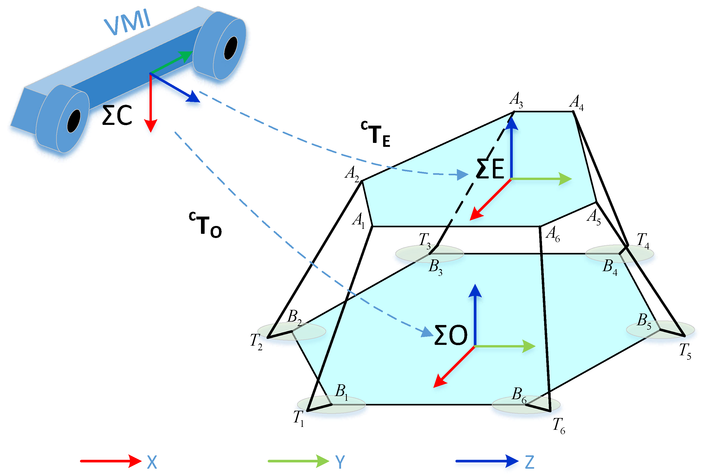
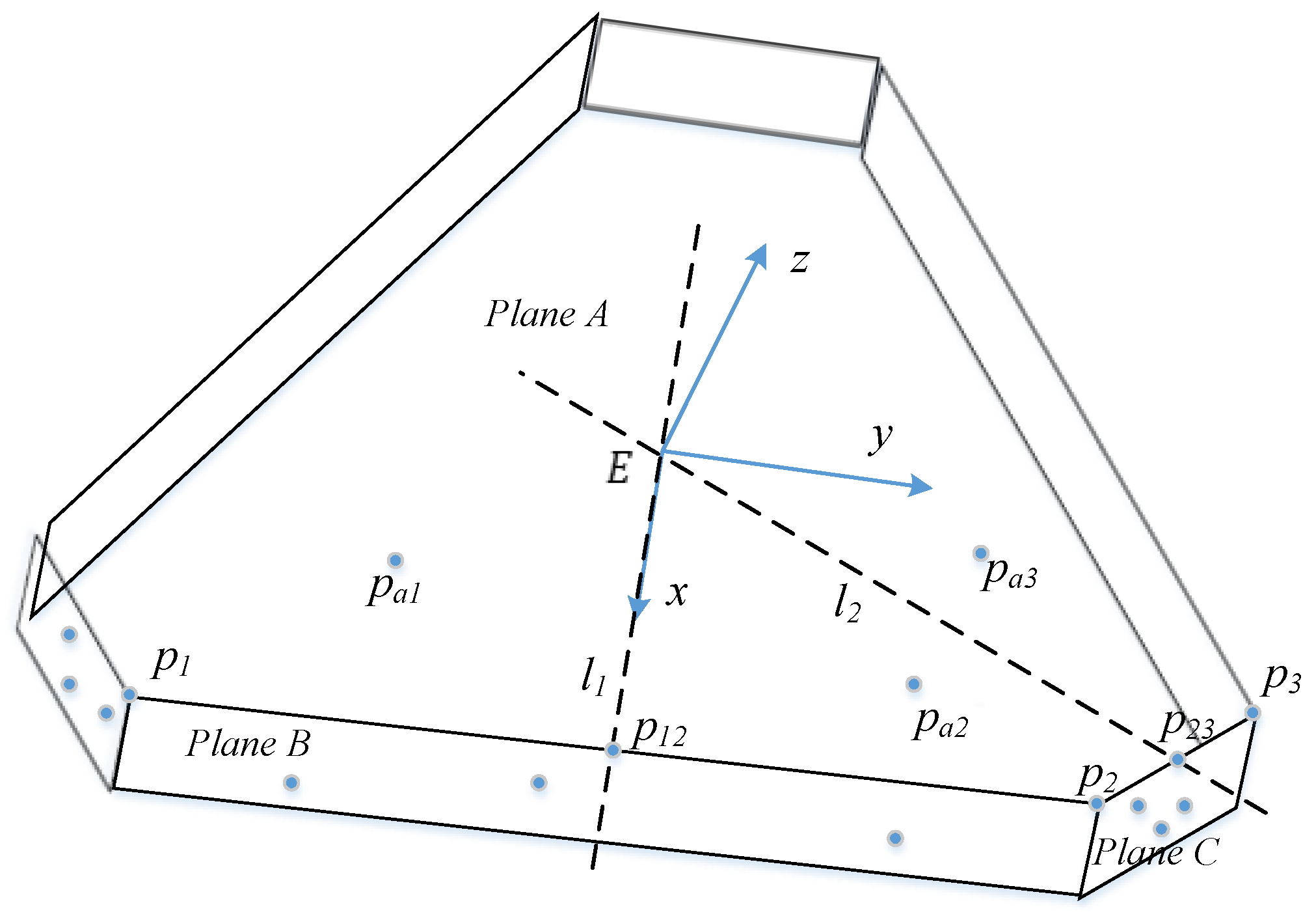
3.1. Pose Estimation Using Optical CMM

As shown in Figure 2, a dual-camera optical CMM C-track 780 is employed to measure the pose of end-effector for the identification of the dynamic model in this research. The pose measurement principle of the optical CMM sensor is presented in this subsection. The target reflectors are taken as the point features. The homogeneous coordinates of the reflectors w.r.t. the sensor frame can be obtained by using triangulation principle [34]. Given a group of non-collinear reflectors $p_i(i=1,2,\dots ,n)$ attached on the end-effector platform, the homogeneous coordinates in the sensor frame can be measured and denoted as ${}^C{\mathbf{P}}_i={[x_{pi},y_{pi},z_{pi},\mathbf{1}]}^T$. In addition, the homogeneous coordinates of the reflectors w.r.t. the end-effector frame $\Sigma E$ denoted as $E{\mathbf{P}}_i=(E{x}_i,E{y}_i,E{z}_i,\mathbf{1})$ are known from the definition of the end-effector frame $\Sigma E$. Correspondingly, the transformation equation of ith feature point can be written as:

$$\begin{array}{cc}\hfill C{\mathbf{P}}_i& =C{\mathbf{T}}_{E}E{\mathbf{P}}_i,\hfill \end{array}$$

(27)

where $C{\mathbf{T}}_E$ is the homogeneous transformation matrix mapping from $\Sigma E$ to $\Sigma C$. In order to derive $C{\mathbf{T}}_E$, at least three non-collinear feature points are required [35]. However, as indicated in [36], at least four coplanar feature points are needed for obtaining a unique solution while additional non-coplanar feature points can be used to improve the estimation accuracy with measurement noise. Similarly, the homogeneous transformation matrix mapping from $\Sigma O$ to $\Sigma C$, $C{\mathbf{T}}_O$, can be derived. Then the pose of the end-effector frame w.r.t. the base frame, ${\mathit{\chi }}_{\mathit{E}}$, can be obtained from the homogeneous transformation matrix $O{\mathbf{T}}_E$ given by Equation (28).

$$\begin{array}{cc}\hfill O{\mathbf{T}}_E& =C{\mathbf{T}}_O^{-1}C{\mathbf{T}}_E.\hfill \end{array}$$

(28)

By using the proprietary software VXelements provided by Creaform Inc., the target frames can be defined based on the selected reflectors on the surface of the end-effector and base frame respectively. The real-time position and rotation information of the end-effector frame w.r.t. the base frame can be acquired, recorded or displayed simultaneously. In addition, the computation associated with the pose estimation of the target frame is carried out by VXelements.

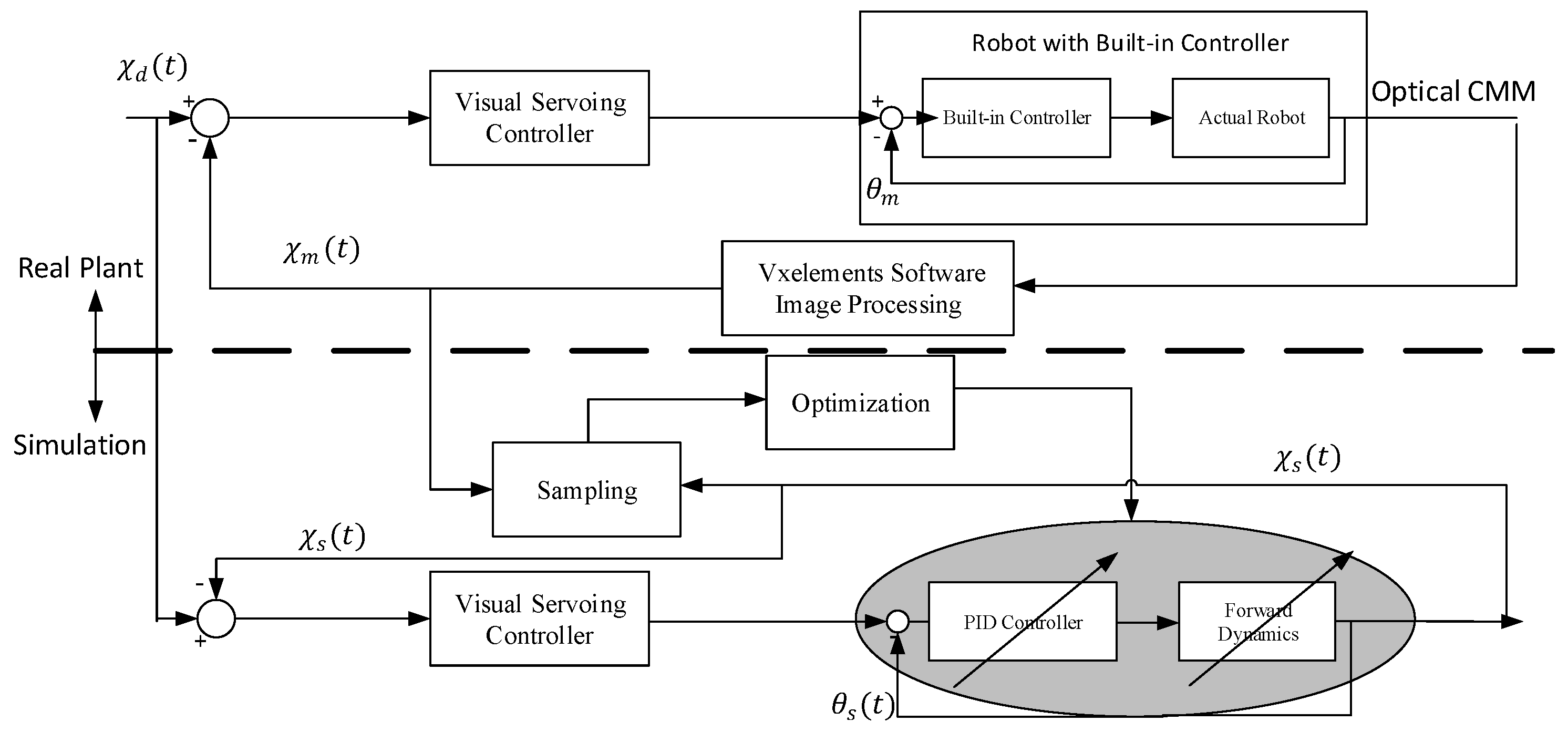
3.2. Closed-Loop Output-Error Identification Method

The basic idea of output error identification is to use nonlinear optimization technique to minimize the squared error between the output of the real plant and the simulated model. Since the motor torque is unaccessible, the pose of the end-effector, ${\mathit{\chi }}_{\mathit{E}}$, measured by optical CMM is used as the output of the system. Hence the closed-loop output-error identification method is adopted [19]. In conventional closed-loop output-error identification method, the controllers should be exactly known and applied to both the real plant and the simulated model. However for an industrial robot, the built-in controllers are usually unknown and need to be identified.

The closed-loop output-error identification approach for vision based robotic system, as depicted in Figure 3, is proposed in this paper. For the built-in controller of the 6-RSS parallel robot, a PID controller is used to control the joint angle of each revolute joint. However the three gains of PID controller are unknown and needed to be identified. During the process of identification, the gains and dynamic parameters are updated in each iteration of nonlinear optimization, which may make the simulated model unstable. Hence, an outer loop visual servoing controller is added to stabilize both real robot and simulated model. The visual servoing controller and the built-in controller construct a cascade PID controller. As stated in [37,38], the cascade controller yields better dynamic performance in terms of stability and working frequency compared with single loop controller. With a well-tuned outer loop visual servoing controller, both the real and simulation systems can have a better performance and stability.

In Figure 3, for both the real plant and simulated model, the same exciting trajectory is given as the input ${\mathit{\chi }}_{\mathit{d}}\left(\mathit{t}\right)$. Then the outer loop visual servoing controller is designed as Equation (30). The inverse kinematic Jacobian $J_{\theta }$ is used to transform the velocity in operational space to that in joint space. By combining Equations (2) and (8), Jacobian matrix $J_{\theta }$ is derived as shown in Equation (29) and the joint position control signal ${\mathit{U}}_{\mathit{\theta }}\left(\mathit{t}\right)$ is generated as shown in Equation (30).

$$\dot{\mathit{\theta }}=J_{ad}\left[\begin{array}{cc}{E}_{3\times 3}& {\mathbf{0}}_{3\times 3}\\ {\mathbf{0}}_{3\times 3}& J_e\end{array}\right]{\dot{\mathit{\chi }}}_{\mathit{E}}=J_{\theta }{\dot{\mathit{\chi }}}_{\mathit{E}}.$$

(29)

$$\begin{array}{cc}\hfill {\mathit{U}}_{\mathit{\theta }}\left(\mathit{t}\right)=& J_{\theta }[k_p({\mathit{\chi }}_{\mathit{d}}\left(\mathit{t}\right)-{\mathit{\chi }}_{\mathit{m}}\left(\mathit{t}\right))+k_d({\dot{\mathit{\chi }}}_{\mathit{d}}\left(\mathit{t}\right)-{\dot{\mathit{\chi }}}_{\mathit{m}}\left(\mathit{t}\right))+k_i\int ({\mathit{\chi }}_{\mathit{d}}\left(\mathit{t}\right)-{\mathit{\chi }}_{\mathit{m}}\left(\mathit{t}\right))dt],\hfill \end{array}$$

(30)

where $k_i,k_p,k_d$ are constants, and ${\mathit{\chi }}_{\mathit{m}}\left(\mathit{t}\right)$ is the visual feedback obtained from VXelements software, while in the simulation ${\mathit{\chi }}_{\mathit{m}}\left(\mathit{t}\right)$ is replaced by ${\mathit{\chi }}_{\mathit{s}}\left(\mathit{t}\right)$ which is the pose calculated by using the forward dynamic model.

In addition, then the PID controller, given in Equation (31), is used to describe the built-in joint controller in each joint and is employed in the simulated model.

$$\begin{array}{c}\hfill {\mathit{\tau }}_{\mathit{a}}\left(t\right)=l_p({\mathit{U}}_{\mathit{\theta }}\left(\mathit{t}\right)-{\mathit{\theta }}_{\mathit{s}}\left(\mathit{t}\right))+l_d({\dot{\mathit{U}}}_{\mathit{\theta }}\left(\mathit{t}\right)-{\dot{\mathit{\theta }}}_{\mathit{s}}\left(\mathit{t}\right))+l_i\int ({\mathit{U}}_{\mathit{\theta }}\left(\mathit{t}\right)-{\mathit{\theta }}_{\mathit{s}}\left(\mathit{t}\right))dt,\end{array}$$

(31)

where $l_i,l_p,l_d$ are the PID parameters to be identified, and ${\mathit{\theta }}_{\mathit{s}}\left(\mathit{t}\right)$ is the joint positions, which can be obtained by analytically solving the inverse kinematics.

The real plant output ${\mathit{Y}}_{\mathit{m}}={[{\mathit{\chi }}_{\mathit{m}}\left(\mathbf{1}\right),{\mathit{\chi }}_{\mathit{m}}\left(\mathbf{2}\right),\cdots ,{\mathit{\chi }}_{\mathit{m}}\left(\mathit{k}\right),]}^T$ and the simulation output ${\mathit{Y}}_{\mathit{s}}={[{\mathit{\chi }}_{\mathit{s}}\left(\mathbf{1}\right),{\mathit{\chi }}_{\mathit{s}}\left(\mathbf{2}\right),\cdots ,{\mathit{\chi }}_{\mathit{s}}\left(\mathit{k}\right)]}^T$ are fed to the optimization process. The parameters to be identified, $\mathsf{\Lambda }$, can be denoted as $\mathsf{\Lambda }={[{\mathsf{\Xi }}^T,l_p,l_i,l_d]}^T$. Accordingly the identification of $\mathsf{\Lambda }$ can be converted to solving the following nonlinear optimization problem:

$$Minimize\Phi \left(\mathsf{\Lambda }\right)=\parallel {\mathit{Y}}_{\mathit{m}}-{\mathit{Y}}_{\mathit{s}}\parallel {}^2.$$

(32)

Then the updating formula for $\mathsf{\Lambda }$ is given as follows:

$${\mathsf{\Lambda }}^{r+1}={\left(J_{\Phi }^T{J}_{\Phi }\right)}^{-1}{J}_{\Phi }^T\Phi \left({\mathsf{\Lambda }}^r\right)+{\mathsf{\Lambda }}^r$$

(33)

where ${\mathsf{\Lambda }}^r$ is the value of $\mathsf{\Lambda }$ in the rth iteration and $J_{\Phi }$ is the Jacobian matrix of $\Phi \left(\mathsf{\Lambda }\right)$ w.r.t. $\mathsf{\Lambda }$ given as:

$$\begin{array}{cc}\hfill J_{\Phi }& =\left[\begin{array}{cccc}\frac{\partial \Phi \left(\mathsf{\Lambda }\right)}{\partial {\mathsf{\Lambda }}_{\mathbf{1}}}& \frac{\partial \Phi \left(\mathsf{\Lambda }\right)}{\partial {\mathsf{\Lambda }}_{\mathbf{2}}}& \cdots & \frac{\partial \Phi \left(\mathsf{\Lambda }\right)}{\partial {\mathsf{\Lambda }}_{\mathbf{67}}}\end{array}\right],\hfill \end{array}$$

(34)

where ${\mathsf{\Lambda }}_{\mathit{i}}$ denotes the ith column of $\mathsf{\Lambda }$. The terminate criteria is given as:

$$\begin{array}{c}{\displaystyle \frac{\Vert \Phi \left({\mathsf{\Lambda }}^{r+1}\right)-\Phi \left({\mathsf{\Lambda }}^r\right)\Vert }{\Vert \Phi \left({\mathsf{\Lambda }}^r\right)\Vert }}\le to{l}_1\hfill \\ \underset{i=1,\cdots ,n}{max}\left|{\displaystyle \frac{{\mathsf{\Lambda }}_i^{r+1}-{\mathsf{\Lambda }}_i^r}{{\mathsf{\Lambda }}_i^r}}\right|\le to{l}_2,\hfill \end{array}$$

(35)

where $|·|$ denotes the absolute-value norm operation, $to{l}_1$ and $to{l}_2$ are the thresholds to be chosen for tuning the accuracy. A compromise should be made between the convergence speed and accuracy when choosing thresholds. To achieve good results in solving the nonlinear optimization problem, a proper initial guess of $\mathsf{\Lambda }$ is needed. For the dynamic parameters of the parallel robots, the initial guess can be calculated from manufacturer specifications. Then a priori PID parameters are obtained based on the simulation model.

3.3. Modified Exciting Trajectory

The exciting trajectories for the dynamic model identification of the serial robots based on the inverse dynamic model have been well studied in [39]. The Finite Fourier series-based exciting trajectory has been tested in a large amount of research works for identification purpose [40]. For serial robots, it can be represented by the following:

$$\begin{array}{cc}{\theta }_i\left(t\right)\hfill & =\sum _{l=1}^n[\frac{sin\left(2\pi f_{0}lt\right)}{2\pi f_{0}l}{s}_i^l-\frac{cos\left(2\pi f_{0}lt\right)}{2\pi f_{0}l}{c}_i^l]+{\theta }_{0_i}\hfill \\ \hfill {\dot{\theta }}_i\left(t\right)& =\sum _{l=1}^n[cos\left(2\pi f_{0}lt\right)s_i^l+sin\left(2\pi f_{0}lt\right)c_i^l]\hfill \\ \hfill {\ddot{\theta }}_i\left(t\right)& =\sum _{l=1}^n[-2\pi f_{0}lsin\left(2\pi f_{0}lt\right)s_i^l+2\pi f_{0}ltcos\left(2\pi f_{0}lt\right)c_i^l],\hfill \end{array}$$

(36)

where ${\theta }_i\left(t\right)$ is the ith joint angle trajectory of serial robots, n is the harmonics number, $f_0$ is the fundamental frequency, and $s_i^l$, $c_i^l$, ${\theta }_{0_i}$ are the trajectory parameters to be optimized. Instead of choosing the joint space states $(\mathit{\theta },\dot{\mathit{\theta }},\ddot{\mathit{\theta }})$ for serial robots, the pose in the operational space is used for the dynamic identification of parallel robots. A modified Finite Fourier series-based exciting trajectory for parallel robots is proposed as:

$$\begin{array}{cc}\hfill {\chi }_i\left(t\right)& =\sum _{l=1}^n[\frac{sin\left(2\pi {\omega }_{0}lt\right)}{2\pi {\omega }_{0}l}{s}_i^l-\frac{cos\left(2\pi {\omega }_{0}lt\right)}{2\pi {\omega }_{0}l}{c}_i^l]+{\chi }_{0_i}\hfill \end{array}$$

(37)

where ${\chi }_i\left(t\right)$ is the ith column of the pose trajectory. Therefore $2n+1$ parameters ${\mathit{\delta }}_{\mathit{i}}={[s_i^1,c_i^1,\cdots ,s_i^n,c_i^n,{\chi }_{0_i}]}^T$ can be estimated by solving a nonlinear optimization problem. The singularity check should be implemented for each sampled pose. According to previous research work [31,41], the maximum wrench rotation range inside the singularity-free domain of the 6-RSS parallel robot is $(-0.9948$ rad, $0.9948$ rad). The inverse kinematic model is used to map the poses into the joint space and to check if the joint angles stay inside the singularity-free domain. To obtain the operational space states in the regression matrix H, the time derivatives of the Euler-angle should be converted to the angular velocity and acceleration, as shown in Equations (2) and (38).

$$\begin{array}{c}\hfill \dot{\mathit{\omega }}=\left[\begin{array}{c}\ddot{\alpha }+\ddot{\gamma }s\beta +\dot{\beta }\dot{\gamma }c\beta \\ c\alpha (\ddot{\beta }-\dot{\alpha }\dot{\gamma }c\beta )+s\alpha (\dot{\beta }\dot{\gamma }s\beta -\dot{\beta }\dot{\alpha }-\ddot{\gamma }c\beta )\\ s\alpha (\ddot{\beta }-\dot{\alpha }\dot{\gamma }c\beta )+c\alpha (\dot{\beta }\dot{\alpha }+\ddot{\gamma }c\beta -\dot{\beta }\dot{\gamma }s\beta )\end{array}\right].\end{array}$$

(38)

As shown in Equation (26), the observability index of H should be maximized to achieve a good identification result for given the exciting trajectories. The observability index $O_{in}$ used in [31] is chosen as the criteria. Therefore the optimal exciting trajectory can be obtained by solving the following nonlinear optimization problem:

$$\begin{array}{c}\hfill Maximize{O}_{in}\left(\delta \right)={\displaystyle \frac{{}^{\varsigma }\sqrt{{\sigma }_1{\sigma }_2\cdots {\sigma }_{\varsigma }}}{\sqrt{m}}}={\displaystyle \frac{{}^{\varsigma }\sqrt{det(\sqrt{H^{T}H}})}{\sqrt{m}}}\end{array}$$

(39)

where the singular values of H are denoted by ${\sigma }_1\ge {\sigma }_2\ge \cdots \ge {\sigma }_{\varsigma }$, m is the number of sampled poses of the trajectory, $\varsigma$ is the number of dynamic parameters to be identified.

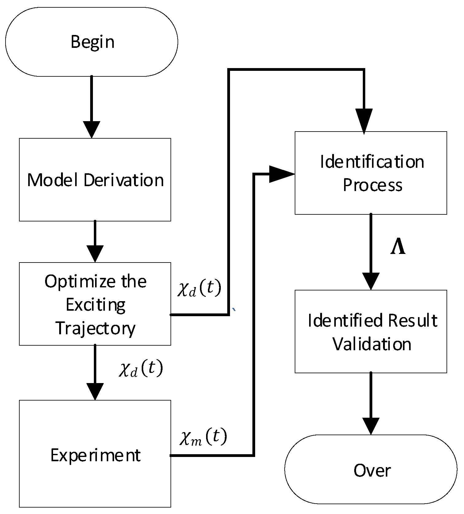
3.4. The Procedure of Identification

The whole procedure of the proposed closed-loop output-error identification method is given in Figure 4. Firstly, the dynamic model of the parallel robot is derived as Equations (17) and (25). Then the optimized exciting trajectory, ${\mathit{\chi }}_{\mathit{d}}\left(t\right)$, can be generated by using the method mentioned in previous subsection. By using $\mathit{\chi }\left(t\right)$ as reference input signal to the outer loop visual servoing control systems of both the real plant and the simulated model, the measured output pose ${\mathit{\chi }}_{\mathit{m}}\left(t\right)$ of the parallel robot by the optical CMM sensor is compared with that of the simulated model. The identification of the parameters $\mathsf{\Lambda }$ is carried out by solving the nonlinear optimization problem. Lastly, the identified model can be validated by feeding several testing trajectories to the systems.

4. Simulation and Experiment Results

In this section, the dynamic model is verified by the simulation using Matlab/SimMechanics. In addition, the closed-loop output-error identification is carried out on a 6-RSS parallel robot. An outer loop visual servoing controller is implemented on the real plant and the simulated model individually. The C-track 780 from Creaform Inc. is adopted to measure the pose of the end-effector of parallel robot.

4.1. Model Validation

The analytical dynamic model is rather complex and it is a non-trival task to ensure that the code of dynamic model is mistake free. A simulation verification method is used to verify the built mathematical dynamic model. A mechanical model of the 6-RSS parallel robot is built by using the Multibody SimMechanics Toolbox of Matlab/Simulink. The SimMechanics model is constructed by choosing the parts from SimMechanics library as shown in Figure 5. The coordinates frames and physical parameters of rigid body blocks can be specified in the setting option. The revolute and spherical joints are used to connect the rigid bodies. The body sensor part can provide the position and orientation of the coordinate frames. The entire model is directly actuated by the torque of the motors, and 3D animation shown in Figure 6 can be provided by SimMechanics. It should be noted that SimMechanics model can only simulate the forward dynamics and cannot be used for controller design. However, it is relatively easy and intuitive to build SimMechanics model with high fidelity [42]. To validate the mathematical dynamic model Equation (17), the explicit form of the forward dynamic model obtained by Equation (40) is employed to compare with the SimMechanics model.

$${\dot{\mathit{v}}}_{\mathit{E}}=M{\left({\mathit{\chi }}_{\mathit{E}}\right)}^{-1}({\mathit{\tau }}_{\mathit{g}}-C({\mathit{\chi }}_{\mathit{E}},{\mathit{v}}_{\mathit{E}}){\mathit{v}}_{\mathit{E}}-G\left({\mathit{\chi }}_{\mathit{E}}\right)-{\mathit{\tau }}_{\mathit{f}}),$$

(40)

The mathematical dynamic model is built by using S-function of Simulink. The initial dynamic model parameters of both SimMechanics and mathematical models are derived from manufacturer specifications and are given in

Table 1. Initial dynamic model parameters of 6-RSS parallel robot.

Dynamic Model Parameters	Initial Value
$m_p$$\left(\mathrm{kg}\right)$	24.0
$I_{x_p}$${10}^{-2}\left(\mathrm{kg}·{\mathrm{m}}^2\right)$	17.8
$I_{y_p}$${10}^{-2}\left(\mathrm{kg}·{\mathrm{m}}^2\right)$	17.8
$I_{z_p}$${10}^{-2}\left(\mathrm{kg}·{\mathrm{m}}^2\right)$	35.0
$m_{wi}$${10}^{-2}\left(\mathrm{kg}\right)$	68.5
$I_{x_{w_i}}$${10}^{-5}\left(\mathrm{kg}·{\mathrm{m}}^2\right)$	22.9
$I_{y_{w_i}}$${10}^{-5}\left(\mathrm{kg}·{\mathrm{m}}^2\right)$	22.9
$I_{z_{w_i}}$${10}^{-5}\left(\mathrm{kg}·{\mathrm{m}}^2\right)$	60.5
$m_{li}$$\left(\mathrm{kg}\right)$	1.31
$I_{x_{l_i}}$${10}^{-5}\left(\mathrm{kg}·{\mathrm{m}}^2\right)$	52.3
$I_{y_{l_i}}$${10}^{-5}\left(\mathrm{kg}·{\mathrm{m}}^2\right)$	52.3
$I_{z_{l_i}}$${10}^{-4}\left(\mathrm{kg}·{\mathrm{m}}^2\right)$	21.3

.

As shown in Figure 7, a simple PID controller is used to stabilize both mathematical and SimMechanic models with the same PID gains. The exciting trajectory ${\mathit{\chi }}_{\mathit{d}}\left(\mathit{t}\right)$ derived from Equation (36) is used as the reference input signal. The outputs of the SimMechanics and mathematical dynamic model (Equation (40)) are ${\mathit{\chi }}_{\_\mathit{s}}\left(\mathit{t}\right)$ and ${\mathit{\chi }}_{\_\mathit{m}}\left(\mathit{t}\right)$ respectively. The difference between ${\mathit{\chi }}_{\_\mathit{s}}\left(\mathit{t}\right)$ and ${\mathit{\chi }}_{\_\mathit{m}}\left(\mathit{t}\right)$ is shown in Figure 8. The maximum position and angle errors are around $1.25$ mm and $3.25\times {10}^{-3}$ rad, which occur at the beginning of the simulation, and are often caused by the kinematic error. The largest steady-state errors are about $0.1$ mm in the position and $0.25\times {10}^{-3}$ rad in the angle, which can prove the correctness of the mathematical model. The validated mathematical model can be used in the simulation part for the subsequent identification.

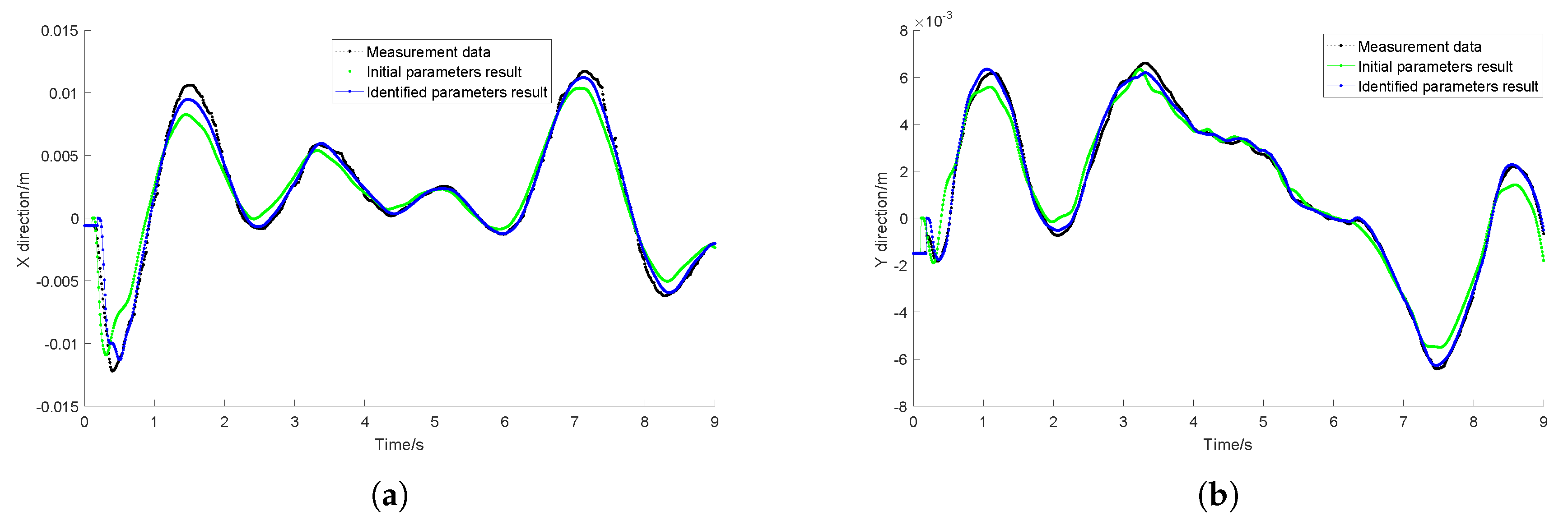
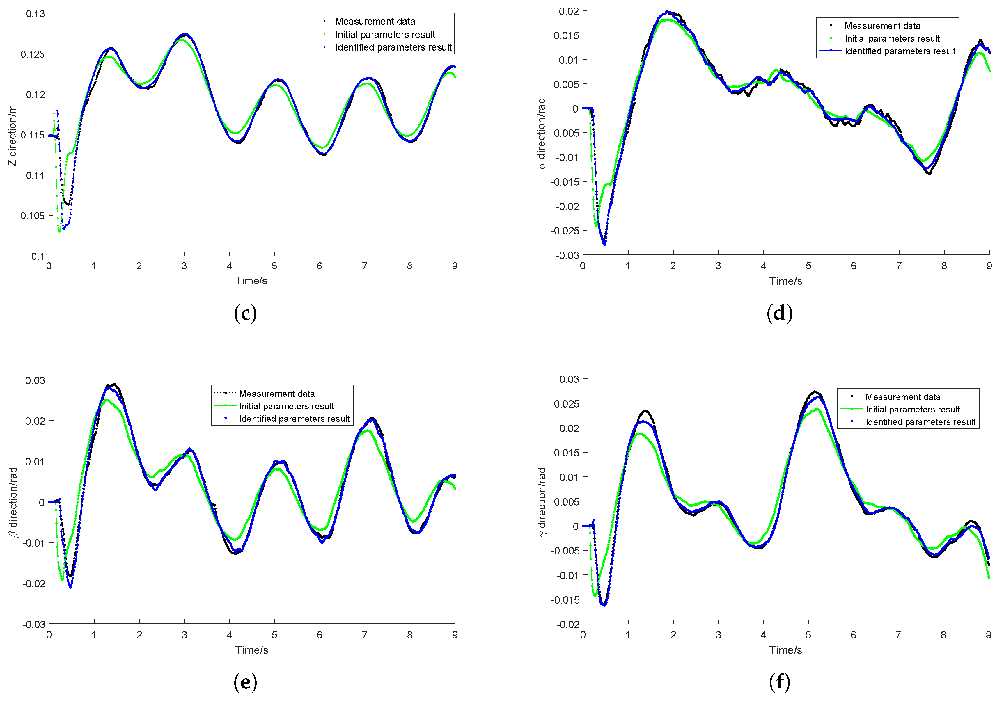
4.2. Identification Experiment

The experiment setup is shown in Figure 9. The 6-RSS parallel robot with 6 built-in joint controllers is provided by Servo & Simulation Inc. (Sanford, FL, USA). The built-in controllers communicate with the robot control computer through two Quanser MultiQ-PCI (Sensoray Model 626) data acquisition cards provided by Quanser Inc. (Markham, ON, Canada). Quanser’s QUARC${}^{TM}$ software is running on the robot control computer with Windows 7.0 32-bit operating system and Intel Core Processor i7-3770 3.4 GHz. QUARC${}^{TM}$ software is capable of generating real-time application though Simulink based controllers and implementing the application in real time on the Windows target. The C-track 780 provided by Creaform Inc. (Levis, QC, Canada) is used to obtain the image data of the reflectors attached on the robot. The reflectors provided by Creaform Inc. are magnetic stickers which are easily fixed on the robots and are used as the feature points. In another Windows 7.0 64-bit computer with Intel Xeon Processor E5-1650 v3 3.5 GHz and NVIDIA Quadro K2200 (Santa Clara, CA, USA) professional graphics board, Vxelements software is used to process the image data and transmit the pose of the end-effector to the robot control computer.

As shown in Figure 10, the reflectors are stuck on the surface of the moving platform. At least three non-collinear points on each plane of Plane A, Plane B and Plane C are employed to build up the equations of planes based on Cramer’s rule. Then the intersection lines and points of three planes can be used to define the x direction of $\Sigma E$, and z direction is aligned with the norm of Plane A. The origin point of $\Sigma E$ is derived from the intersection point of $l_1$ and $l_2$. Then, the obtained $\Sigma E$ in the optical CMM sensor frame is directly used as the target frame. The base frame of the parallel robot is defined by following the similar procedure.

To eliminate the high frequency noise of the pose measurement from the optical CMM, measurement data is filtered by the zero-phase forward and reverse 8th order Butterworth filter with the cut-off frequency 60 Hz. The filtering process is carried out by the Zero-phase digital filtering function of Maltab, $filtfilt$.

The optimization of the exciting trajectory is carried out by using the $GA$ function of the Optimization Toolbox of Matlab. The GA algorithm uses binary code to represent the harmonic parameters. The fundamental frequency $f_0$ is selected as $0.1$ Hz and the harmonics number n is chosen as 5. By taking the observation index as the fitness function, the binary code is updated to maximize the fitness value in each step. The starting value of the observation index $O_{in}$ is $0.38$ and the stop criteria is set as ${10}^{-10}$. The algorithm stops after 324 iterations with the maximum $O_{in}$$1.345$. The derived optimal exciting trajectory is given in Figure 11.

The identification procedure is implemented off-line through simulation illustrated in Section 3.2. The optimization procedure is carried out by using optimization functions in Matlab R2016a. The minimal performance requirements of the computation platform are given as: 4 cores Inter or AMD Processor; 6 GB disk space; 4 GB RAM. The same outer loop visual servoing controller, Equation (30), is employed in the simulation. The gains of the visual servoing controller are obtained through trial and error in the extensive experimental tests. The well-tuned gains are given as $k_p=0.3,k_d=0.001,k_i=2.4$. and the built-in joint PID controllers, Equation (31), are also implemented in the simulation. The dynamic parameters derived from manufacturer specifications are used as initial values, and the initial values of the PID gains in Equation (31) are obtained through trial and error based on the simulation model. During the tuning, in the simulation system, the inertial and friction parameters are set as the values based on the manufacturer specifications, and the visual servoing controller gains are set as the same values of the controller of the real system. The identified parameters, given in

Table 2. Identified parameters of 6-RSS parallel robot.

Parameters	Initial Value	Identified Value	Parameters	Initial Value	Identified Value
$m_p$$\left(\mathrm{kg}\right)$	24.0	23.5	$m_{l4}$$\left(\mathrm{kg}\right)$	1.31	1.24
$I_{x_p}$${10}^{-2}\left(\mathrm{kg}·{\mathrm{m}}^2\right)$	17.8	16.1	$I_{x_{l_4}}$${10}^{-5}\left(\mathrm{kg}·{\mathrm{m}}^2\right)$	52.3	12.9
$I_{y_p}$${10}^{-2}\left(\mathrm{kg}·{\mathrm{m}}^2\right)$	17.8	14.4	$I_{y_{l_4}}$${10}^{-5}\left(\mathrm{kg}·{\mathrm{m}}^2\right)$	52.3	39.2
$I_{z_p}$${10}^{-2}\left(\mathrm{kg}·{\mathrm{m}}^2\right)$	35.0	33.7	$m_{l5}$$\left(\mathrm{kg}\right)$	1.31	1.33
$m_{w1}$${10}^{-2}\left(\mathrm{kg}\right)$	68.5	67.1	$I_{x_{l_5}}$${10}^{-5}\left(\mathrm{kg}·{\mathrm{m}}^2\right)$	52.3	30.7
$I_{z_{w_1}}$${10}^{-5}\left(\mathrm{kg}·{\mathrm{m}}^2\right)$	60.5	69.4	$I_{y_{l_5}}$${10}^{-5}\left(\mathrm{kg}·{\mathrm{m}}^2\right)$	52.3	49.7
$m_{w2}$${10}^{-2}\left(\mathrm{kg}\right)$	68.5	68.7	$m_{l6}$$\left(\mathrm{kg}\right)$	1.31	1.34
$I_{z_{w_2}}$${10}^{-5}\left(\mathrm{kg}·{\mathrm{m}}^2\right)$	60.5	10.0	$I_{x_{l_6}}$${10}^{-5}\left(\mathrm{kg}·{\mathrm{m}}^2\right)$	52.3	47.0
$m_{w3}$$\left(\mathrm{kg}\right)$${10}^{-2}\left(\mathrm{kg}\right)$	68.5	68.0	$I_{y_{l_6}}$${10}^{-5}\left(\mathrm{kg}·{\mathrm{m}}^2\right)$	52.3	50.9
$I_{z_{w_3}}$${10}^{-5}\left(\mathrm{kg}·{\mathrm{m}}^2\right)$	60.5	22.6	$f_{c_1}$	0	0.104
$m_{w4}$${10}^{-2}\left(\mathrm{kg}\right)$	68.5	67.7	$f_{v_1}$	0	0.148
$I_{z_{w_4}}$${10}^{-5}\left(\mathrm{kg}·{\mathrm{m}}^2\right)$	60.5	76.0	$f_{c_2}$	0	0.111
$m_{w5}$$\left(\mathrm{kg}\right)$${10}^{-2}\left(\mathrm{kg}\right)$	68.5	68.3	$f_{v_2}$	0	0.187
$I_{z_{w_5}}$${10}^{-5}\left(\mathrm{kg}·{\mathrm{m}}^2\right)$	60.5	44.1	$f_{c_3}$	0	0.0336
$m_{w6}$$\left(\mathrm{kg}\right)$${10}^{-2}\left(\mathrm{kg}\right)$	68.5	68.4	$f_{v_3}$	0	0.0993
$I_{z_{w_6}}$${10}^{-5}\left(\mathrm{kg}·{\mathrm{m}}^2\right)$	60.5	69.6	$f_{c_4}$	0	0.147
$m_{l1}$$\left(\mathrm{kg}\right)$	1.31	1.33	$f_{v_4}$	0	0.854
$I_{x_{l_1}}$${10}^{-5}\left(\mathrm{kg}·{\mathrm{m}}^2\right)$	52.3	63.0	$f_{c_5}$	0	0.104
$I_{y_{l_1}}$${10}^{-5}\left(\mathrm{kg}·{\mathrm{m}}^2\right)$	52.3	68.4	$f_{v_5}$	0	0.0803
$m_{l2}$$\left(\mathrm{kg}\right)$	1.31	1.32	$f_{c_6}$	0	0.0828
$I_{x_{l_2}}$${10}^{-5}\left(\mathrm{kg}·{\mathrm{m}}^2\right)$	52.3	60.7	$f_{v_6}$	0	0.0349
$I_{y_{l_2}}$${10}^{-5}\left(\mathrm{kg}·{\mathrm{m}}^2\right)$	52.3	71.8	$l_p$	10	10.5
$m_{l3}$$\left(\mathrm{kg}\right)$	1.31	1.25	$l_i$	12	11.4
$I_{x_{l_3}}$${10}^{-5}\left(\mathrm{kg}·{\mathrm{m}}^2\right)$	52.3	22.4	$l_d$	0.1	0.164
$I_{y_{l_3}}$${10}^{-5}\left(\mathrm{kg}·{\mathrm{m}}^2\right)$	52.3	35.5

, are derived by using $lsqnonlin$ function of the Optimization Toolbox of Matlab after 8 iterations. A total of 50 out of 67 parameters are identified, and are used in the simulation model, Equation (40), to capture the dynamic characteristic of the parallel robot. The other parameters either do not contribute to or have slight impact on the dynamics of the parallel robot. Those parameters can be eliminated by using QR decomposition on the regression matrix H [23,43]. If any diagonal elements of $\underline{\mathit{R}}$ are smaller than the pre-defined small number, i.e., $R_{ii}<\epsilon$, where $\epsilon$ is chosen as ${10}^{-3}$ in the paper, the corresponding columns of the regression matrix H are deleted. By doing so, the matrix H is better conditioned and the identification procedure is sped up.

Then, the pose trajectories are generated by using the identified parameters in the simulation, and are compared with the pose measurement, as shown in Figure 12.

Table 3. The RMS levels of the pose trajectory errors.

	Before Identification	After Identification
x direction (mm)	1.26	0.408
y direction (mm)	1.16	0.235
z direction (mm)	1.55	0.494
$\alpha$ direction ${10}^{-3}$ (rad)	2.52	0.956
$\beta$ direction ${10}^{-3}$ (rad)	3.58	0.797
$\gamma$ direction ${10}^{-3}$ (rad)	2.80	0.725

shows the root-mean-square (RMS) levels of the pose trajectory errors.

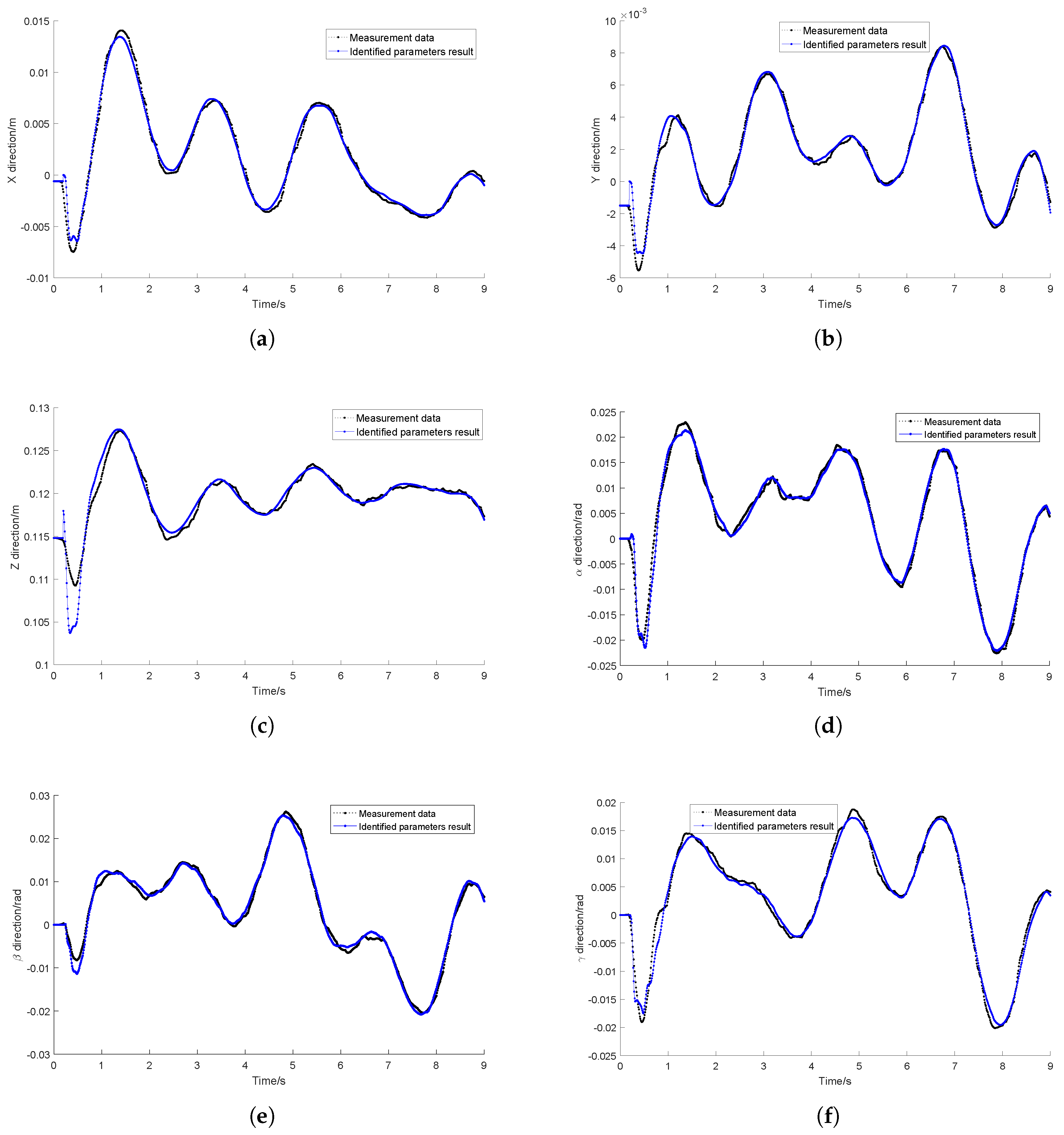
4.3. Identified Results Validation

To verify the identified parameters, ten more trajectories are generated according to Equation (36) with random harmonic parameters under the singularity constraint. The generated trajectories are used as desired trajectories, and are fed to the parallel robot and the identified model in the simulation respectively. The RMS levels of the pose trajectory errors are given in

Table 4. The RMS levels of the ten validation trajectory errors.

	x (mm)	y (mm)	z (mm)	$\mathit{\alpha }$${10}^{-3}$ (rad)	$\mathit{\beta }$${10}^{-3}$ (rad)	$\mathit{\gamma }$${10}^{-3}$ (rad)
1st	0.517	0.384	0.709	1.091	0.963	0.966
2nd	0.273	0.410	0.522	1.157	1.071	0.932
3rd	0.381	0.403	0.600	1.242	0.830	1.143
4th	0.341	0.511	0.617	1.136	0.814	1.161
5th	0.322	0.394	0.464	1.219	0.877	0.835
6th	0.310	0.301	0.441	1.195	1.111	1.040
7th	0.360	0.402	0.455	1.263	1.176	1.024
8th	0.418	0.483	0.460	1.251	1.211	1.015
9th	0.342	0.510	0.557	1.411	1.156	0.711
10th	0.318	0.379	0.473	1.219	1.023	0.905

, and the measurement and the simulated pose trajectories are given in Figure 13 according to the 1st desired trajectory. The RMS of the position and orientation errors for all ten trajectories are below $0.8$ mm and $1.4\times {10}^{-3}$ rad respectively, which validate the identified results of previous subsection. In addition, the proposed identification procedure is implemented based on the ten trajectories to analyze the statistic property of the identification results. After deriving ten more groups of identified parameters, the variation measure of the identification results are given in

Table 5. Variation measure of the identification result.

Parameters	Variation Measure	Parameters	Variation Measure
$m_p$$\left(\mathrm{kg}\right)$	$0.48\%$	$m_{l4}$$\left(\mathrm{kg}\right)$	$19.1\%$
$I_{x_p}$$\left(\mathrm{kg}·{\mathrm{m}}^2\right)$	$5.0\%$	$I_{x_{l_4}}$$\left(\mathrm{kg}·{\mathrm{m}}^2\right)$	$0.16\%$
$I_{y_p}$$\left(\mathrm{kg}·{\mathrm{m}}^2\right)$	$24.9\%$	$I_{y_{l_4}}$$\left(\mathrm{kg}·{\mathrm{m}}^2\right)$	$0.06\%$
$I_{z_p}$$\left(\mathrm{kg}·{\mathrm{m}}^2\right)$	$8.6\%$	$m_{l5}$$\left(\mathrm{kg}\right)$	$10.1\%$
$m_{w1}$$\left(\mathrm{kg}\right)$	$0.56\%$	$I_{x_{l_5}}$$\left(\mathrm{kg}·{\mathrm{m}}^2\right)$	$0.15\%$
$I_{z_{w_1}}$$\left(\mathrm{kg}·{\mathrm{m}}^2\right)$	$6.6\%$	$I_{y_{l_5}}$$\left(\mathrm{kg}·{\mathrm{m}}^2\right)$	$0.01\%$
$m_{w2}$$\left(\mathrm{kg}\right)$	$1.5\%$	$m_{l6}$$\left(\mathrm{kg}\right)$	$12.9\%$
$I_{z_{w_2}}$$\left(\mathrm{kg}·{\mathrm{m}}^2\right)$	$1.4\%$	$I_{x_{l_6}}$$\left(\mathrm{kg}·{\mathrm{m}}^2\right)$	$0.17\%$
$m_{w3}$$\left(\mathrm{kg}\right)$	$3.4\%$	$I_{y_{l_6}}$$\left(\mathrm{kg}·{\mathrm{m}}^2\right)$	$0.02\%$
$I_{z_{w_3}}$$\left(\mathrm{kg}·{\mathrm{m}}^2\right)$	$5.0\%$	$f_{c_1}$	$15.9\%$
$m_{w4}$$\left(\mathrm{kg}\right)$	$3.7\%$	$f_{v_1}$	$11.7\%$
$I_{z_{w_4}}$$\left(\mathrm{kg}·{\mathrm{m}}^2\right)$	$3.8\%$	$f_{c_2}$	$21.4\%$
$m_{w5}$$\left(\mathrm{kg}\right)$	$6.6\%$	$f_{v_2}$	$13.9\%$
$I_{z_{w_5}}$$\left(\mathrm{kg}·{\mathrm{m}}^2\right)$	$6.6\%$	$f_{c_3}$	$9.0\%$
$m_{w6}$$\left(\mathrm{kg}\right)$	$0.79\%$	$f_{v_3}$	$16.4\%$
$I_{z_{w_6}}$$\left(\mathrm{kg}·{\mathrm{m}}^2\right)$	$1.7\%$	$f_{c_4}$	$17.8\%$
$m_{l1}$$\left(\mathrm{kg}\right)$	$4.1\%$	$f_{v_4}$	$15.2\%$
$I_{x_{l_1}}$$\left(\mathrm{kg}·{\mathrm{m}}^2\right)$	$0.04\%$	$f_{c_5}$	$15.1\%$
$I_{y_{l_1}}$$\left(\mathrm{kg}·{\mathrm{m}}^2\right)$	$0.11\%$	$f_{v_5}$	$21.8\%$
$m_{l2}$$\left(\mathrm{kg}\right)$	$5.2\%$	$f_{c_6}$	$23.4\%$
$I_{x_{l_2}}$$\left(\mathrm{kg}·{\mathrm{m}}^2\right)$	$0.05\%$	$f_{v_6}$	$13.0\%$
$I_{y_{l_2}}$$\left(\mathrm{kg}·{\mathrm{m}}^2\right)$	$0.12\%$	$l_p$	$2.82\%$
$m_{l3}$$\left(\mathrm{kg}\right)$	$20.9\%$	$l_i$	$0.44\%$
$I_{x_{l_3}}$$\left(\mathrm{kg}·{\mathrm{m}}^2\right)$	$0.09\%$	$l_d$	$3.7\%$
$I_{y_{l_3}}$$\left(\mathrm{kg}·{\mathrm{m}}^2\right)$	$0.17\%$

. The highest relative variation of the parameter is below $25\%$, which is acceptable. It has been stated that less than 30 percent in the variation measure of the parameters gives a good match to the real system [44].

Therefore by using the proposed visual closed-loop output-error identification method, the identified dynamic model can approximate the real plant with acceptable accuracy.

5. Conclusions and Further Works

In this paper, a visual closed-loop output-error identification method based on an optical CMM sensor for parallel robots is proposed. An outer loop visual servoing controller is employed in both the real plant and the simulation model to stabilize the two systems. The benefits of the proposed method are summarized as follows: elimination of the need for the joint and torque measurements, the exact knowledge of the built-in joint controller of the industrial robots, and the time-consuming forward kinematics calculation. The correctness and accuracy of the built dynamic model are validated by the Matlab/SimMechanics simulation. The experimental test results show that the identified dynamic model can capture the dynamics of the real parallel robot with satisfactory accuracy. The proposed method can be easily applied to other types of industrial parallel robots with unknown PID built-in controller or its variant, such as 6 DOF Stewart platforms, 6 UPS and 6 RUS parallel robots etc. The complexity of those dynamic models is similar to that of the 6-RSS parallel robot. Since the analytical solution of the forward kinematics of those 6 DOF parallel robots does not exist, the proposed visual identification method does not need the forward kinematic model and hence has a lot of advantages. The proposed identification method can also be applied to parallel robots with less DOF than 6 DOF. Taking the advantages of the visual sensor, the dynamic model can be identified for the visual servoing purpose. In the future, the advanced model-based visual servoing control method will be further studied to improve the tracking performance of parallel robots based on the identification results.

References

1. Miletović, I.; Pool, D.; Stroosma, O.; van Paassen, M.; Chu, Q. Improved Stewart platform state estimation using inertial and actuator position measurements. Control Eng. Pract. 2017, 62, 102–115. [Google Scholar] [CrossRef] [Green Version]
2. Abdellatif, H.; Heimann, B. Model-Based Control for Industrial Robots: Uniform Approaches for Serial and Parallel Structures. In Industrial Robotics; Cubero, S., Ed.; IntechOpen: Rijeka, Croatia, 2006; Chapter 19; pp. 523–556. [Google Scholar] [CrossRef]
3. Bai, S.; Teo, M.Y. Kinematic calibration and pose measurement of a medical parallel manipulator by optical position sensors. J. Robot. Syst. 2003, 20, 201–209. [Google Scholar] [CrossRef]
4. Absolute Accuracy Industrial Robot Option. 2011. Available online: https://www.google.com.hk/url?sa=t&rct=j&q=&esrc=s&source=web&cd=2&ved=2ahUKEwiK6L_fndLjAhUQTY8KHYTaBjcQFjABegQIChAE&url=https%3A%2F%2Flibrary.e.abb.com%2Fpublic%2F0f879113235a0e1dc1257b130056d133%2FAbsolute%2520Accuracy%2520EN_R4%2520US%252002_05.pdf&usg=AOvVaw2YHKD4M3X8PjRHuBDV8y_F (accessed on 7 November 2018).
5. Taghirad, H.D. Parallel Robots: Mechanics and Control; CRC Press: Boca Raton, FL, USA, 2013. [Google Scholar]
6. Merlet, J.P. Parallel Robots; Springer Science & Business Media: Berlin, Germany, 2012. [Google Scholar]
7. Dasgupta, B.; Mruthyunjaya, T. A Newton-Euler formulation for the inverse dynamics of the Stewart platform manipulator. Mech. Mach. Theory 1998, 33, 1135–1152. [Google Scholar] [CrossRef]
8. Nguyen, C.C.; Pooran, F.J. Dynamic analysis of a 6 DOF CKCM robot end-effector for dual-arm telerobot systems. Robot. Auton. Syst. 1989, 5, 377–394. [Google Scholar] [CrossRef]
9. Wang, J.; Gosselin, C.M. A new approach for the dynamic analysis of parallel manipulators. Multibody Syst. Dyn. 1998, 2, 317–334. [Google Scholar] [CrossRef]
10. Zanganeh, K.E.; Sinatra, R.; Angeles, J. Kinematics and dynamics of a six-degree-of-freedom parallel manipulator with revolute legs. Robotica 1997, 15, 385–394. [Google Scholar] [CrossRef]
11. Dumlu, A.; Erenturk, K. Modeling and trajectory tracking control of 6-DOF RSS type parallel manipulator. Robotica 2014, 32, 643–657. [Google Scholar] [CrossRef]
12. Ljung, L. (Ed.) System Identification (2nd ed.): Theory for the User; Prentice Hall PTR: Upper Saddle River, NJ, USA, 1999. [Google Scholar]
13. Hollerbach, J.; Khalil, W.; Gautier, M. Model identification. In Springer Handbook of Robotics; Springer: Berlin/Heidelberg, Germany, 2016; pp. 113–138. [Google Scholar]
14. Swevers, J.; Verdonck, W.; De Schutter, J. Dynamic model identification for industrial robots. IEEE Control Syst. Mag. 2007, 27, 58–71. [Google Scholar]
15. Wu, J.; Wang, J.; You, Z. An overview of dynamic parameter identification of robots. Robot. Comput.-Integr. Manuf. 2010, 26, 414–419. [Google Scholar] [CrossRef]
16. Calanca, A.; Capisani, L.M.; Ferrara, A.; Magnani, L. MIMO closed loop identification of an industrial robot. IEEE Trans. Control Syst. Technol. 2010, 19, 1214–1224. [Google Scholar] [CrossRef]
17. Olsen, M.M.; Swevers, J.; Verdonck, W. Maximum likelihood identification of a dynamic robot model: Implementation issues. Int. J. Robot. Res. 2002, 21, 89–96. [Google Scholar] [CrossRef]
18. Janot, A.; Vandanjon, P.O.; Gautier, M. An instrumental variable approach for rigid industrial robots identification. Control Eng. Pract. 2014, 25, 85–101. [Google Scholar] [CrossRef]
19. Gautier, M.; Janot, A.; Vandanjon, P.O. A new closed-loop output error method for parameter identification of robot dynamics. IEEE Trans. Control Syst. Technol. 2013, 21, 428–444. [Google Scholar] [CrossRef]
20. Walter, E.; Pronzato, L. Identification of Parametric Models from Experimental Data; Springer: Berlin/Heidelberg, Germany, 1997. [Google Scholar]
21. Del Prete, A.; Mansard, N.; Ramos, O.E.; Stasse, O.; Nori, F. Implementing torque control with high-ratio gear boxes and without joint-torque sensors. Int. J. Humanoid Robot. 2016, 13, 1550044. [Google Scholar] [CrossRef]
22. Brunot, M.; Janot, A.; Young, P.C.; Carrillo, F. An improved instrumental variable method for industrial robot model identification. Control Eng. Pract. 2018, 74, 107–117. [Google Scholar] [CrossRef] [Green Version]
23. Briot, S.; Gautier, M. Global identification of joint drive gains and dynamic parameters of parallel robots. Multibody Syst. Dyn. 2015, 33, 3–26. [Google Scholar] [CrossRef]
24. Grotjahn, M.; Heimann, B.; Abdellatif, H. Identification of friction and rigid-body dynamics of parallel kinematic structures for model-based control. Multibody Syst. Dyn. 2004, 11, 273–294. [Google Scholar] [CrossRef]
25. Abdellatif, H.; Heimann, B. Advanced model-based control of a 6-DOF hexapod robot: A case study. IEEE/ASME Trans. Mechatron. 2010, 15, 269–279. [Google Scholar] [CrossRef]
26. Vivas, A.; Poignet, P.; Marquet, F.; Pierrot, F.; Gautier, M. Experimental dynamic identification of a fully parallel robot. In Proceedings of the 2003 IEEE International Conference on Robotics and Automation (Cat. No. 03CH37422), Taipei, Taiwan, 14–19 September 2003; IEEE: Piscataway, NJ, USA, 2003; Volume 3, pp. 3278–3283. [Google Scholar]
27. Guegan, S.; Khalil, W.; Lemoine, P. Identification of the dynamic parameters of the orthoglide. In Proceedings of the 2003 IEEE International Conference on Robotics and Automation (Cat. No. 03CH37422), Taipei, Taiwan, 14–19 September 2003; IEEE: Piscataway, NJ, USA, 2003; Volume 3, pp. 3272–3277. [Google Scholar]
28. Renaud, P.; Vivas, A.; Andreff, N.; Poignet, P.; Martinet, P.; Pierrot, F.; Company, O. Kinematic and dynamic identification of parallel mechanisms. Control Eng. Pract. 2006, 14, 1099–1109. [Google Scholar] [CrossRef]
29. Lightcap, C.; Banks, S. Dynamic identification of a mitsubishi pa10-6ce robot using motion capture. In Proceedings of the 2007 IEEE/RSJ International Conference on Intelligent Robots and Systems, San Diego, CA, USA, 29 October–2 November 2007; pp. 3860–3865. [Google Scholar]
30. Chellal, R.; Cuvillon, L.; Laroche, E. Model identification and vision-based H∞ position control of 6-DoF cable-driven parallel robots. Int. J. Control 2017, 90, 684–701. [Google Scholar] [CrossRef]
31. Li, P.; Zeng, R.; Xie, W.; Zhang, X. Relative posture-based kinematic calibration of a 6-RSS parallel robot by optical coordinate measurement machine. Int. J. Adv. Robot. Syst. 2018, 15, 1729881418765861. [Google Scholar] [CrossRef]
32. Shu, T.; Gharaaty, S.; Xie, W.; Joubair, A.; Bonev, I.A. Dynamic Path Tracking of Industrial Robots With High Accuracy Using Photogrammetry Sensor. IEEE/ASME Trans. Mechatron. 2018, 23, 1159–1170. [Google Scholar] [CrossRef]
33. Xie, W.; Krzeminski, M.; El-Tahan, H.; El-Tahan, M. Intelligent friction compensation (IFC) in a harmonic drive. In Proceedings of the IEEE NECEC, St. John’s, NL, Canada, 13 November 2002. [Google Scholar]
34. Hartley, R.I.; Sturm, P. Triangulation. Comput. Vis. Image Underst. 1997, 68, 146–157. [Google Scholar] [CrossRef]
35. Wilson, W.J.; Hulls, C.C.W.; Bell, G.S. Relative end-effector control using cartesian position based visual servoing. IEEE Trans. Robot. Autom. 1996, 12, 684–696. [Google Scholar] [CrossRef]
36. Yuan, J.S. A general photogrammetric method for determining object position and orientation. IEEE Trans. Robot. Autom. 1989, 5, 129–142. [Google Scholar] [CrossRef]
37. Brosilow, C.; Joseph, B. Techniques of Model-Based Control; Prentice Hall Professional: Upper Saddle River, NJ, USA, 2002. [Google Scholar]
38. Marlin, T.E. Process Control, Designing Processes and Control Systems for Dynamic Performance. Available online: https://pdfs.semanticscholar.org/c068/dedc943743ce3ee416ba9202a7172b715e3a.pdf (accessed on 27 June 2019).
39. Park, K.J. Fourier-based optimal excitation trajectories for the dynamic identification of robots. Robotica 2006, 24, 625–633. [Google Scholar] [CrossRef]
40. Bona, B.; Curatella, A. Identification of industrial robot parameters for advanced model-based controllers design. In Proceedings of the 2005 IEEE International Conference on Robotics and Automation, Barcelona, Spain, 18–22 April 2005; pp. 1681–1686. [Google Scholar]
41. Zeng, R.; Dai, S.; Xie, W.; Zhang, X. Determination of the proper motion range of the rotary actuators of 6-RSS parallel robot. In Proceedings of the 2015 CCToMM Symposium on Mechanisms, Machines, and Mechatronics, Carleton University, Ottawa, ON, Canada, 28–29 May 2015; pp. 28–29. [Google Scholar]
42. Van Boekel, J. SimMechanics, MapleSim and Dymola: A First Look on Three Multibody Packages. 2009. Available online: https://www.semanticscholar.org/paper/SimMechanics-%2C-MapleSim-and-Dymola- %3A-a-first-look-Boekel/c51909107f1ddb67faf8bda1b387b0659ec04a7f (accessed on 7 November 2018).
43. Gautier, M. Numerical calculation of the base inertial parameters of robots. J. Robot. Syst. 1991, 8, 485–506. [Google Scholar] [CrossRef]
44. Taghirad, H.; Belanger, P. Modeling and parameter identification of harmonic drive systems. J. Dyn. Syst. Meas. Control 1998, 120, 439–444. [Google Scholar] [CrossRef]
Figure 1. (a) The sketch of 6-RSS parallel robot, (b) Single serial branch.
Electronics 08 00836 g001
Figure 2. The pose measurement system of a 6-RSS parallel robot.
Electronics 08 00836 g002
Figure 3. The block diagram of closed-loop control system for model identification of 6-RSS parallel robot.
Electronics 08 00836 g003
Figure 4. Sketch of the identification procedure.
Electronics 08 00836 g004
Figure 5. Mechanical model of 6-RSS parallel robot built by SimMechanics.
Electronics 08 00836 g005
Figure 6. 3D animation of 6-RSS parallel robot. https://youtu.be/HXtCvgkn2jw.
Electronics 08 00836 g006
Figure 7. Dynamic model verification block diagram of 6-RSS parallel robot.
Electronics 08 00836 g007
Figure 8. Simulation results of SimMechanics model. (a) Position error; (b) Angle error.
Electronics 08 00836 g008
Figure 9. Architecture of the Experiment System.
Electronics 08 00836 g009
Figure 10. Measurement of Σ E .
Electronics 08 00836 g010
Figure 11. Optimal exciting trajectory. (a) Positional trajectory; (b) Angular trajectory.
Electronics 08 00836 g011
Figure 12. The pose trajectories of the parallel robot: the measurement of the real plant (black dot), the output of the simulation with initial parameters (green line), the output of the simulation with identified parameters (blue line), (a) Along X Direction; (b) Along Y Direction; (c) Along Z Direction; (d) Around α Axis; (e) Around β Axis; (f) Around γ Axis.
Electronics 08 00836 g012aElectronics 08 00836 g012b
Figure 13. The pose trajectories of the parallel robot: the measurement of the real plant (black dot), the output of the simulation with identified parameters (blue line), (a) Along X Direction; (b) Along Y Direction; (c) Along Z Direction;(d) Around α Axis; (e) Around β Axis; (f) Around γ Axis.
Electronics 08 00836 g013