Embedded Flight Control Based on Adaptive Sliding Mode Strategy for a Quadrotor Micro Air Vehicle


Tecnologico de Monterrey, Escuela de Ingenieria y Ciencias, Monterrey, NL 64849, Mexico
*
Author to whom correspondence should be addressed.
Electronics 2019, 8(7), 793; https://doi.org/10.3390/electronics8070793
Submission received: 14 June 2019
/
Revised: 5 July 2019
/
Accepted: 8 July 2019
/
Published: 16 July 2019
(This article belongs to the Special Issue Motion Planning and Control for Robotics)
Abstract
:The design of an embedded flight controller for a quadrotor micro air vehicle, which is subject to uncertainties and perturbations, is addressed. In order to obtain robustness against bounded uncertainties and disturbances, an adaptive sliding mode controller is proposed. The control adaptive gains allow using only necessary control to satisfy the task, reducing the chattering effect and at the same time reject external perturbations. Furthermore, a stability analysis of the closed-loop system is given. Finally, simulations and experimental results carried out on a commercial micro air vehicle demonstrate the feasibility and advantages of the proposed flight controller.
1. Introduction
The study about Unmanned Aerial Vehicles (UAVs), particularly the quadrotor systems, has grown exponentially, such that many applications have been developed due to their advantages such as vertical take-off and landing, hovering, and maneuverability. Then, quad-rotors are employed in inspection-, mapping-, and surveillance-related tasks. Recently, Micro Air Vehicles (MAVs) (according to the definition in [1], these vehicles have a mass kg and a size m) have attracted attention because they can access confined and denied GPS spaces such as inside buildings, pipelines, halls, factories, schools, and more. Since MAVs are designed to operate in the above places, they require more advanced controllers to achieve the commanded tasks.
Many commercial quadrotors are available on the market. Nonetheless, we focus on the Parrot mini drone rolling spider, which due to its tiny size is classified as an MAV. These drones are safe and reliable, and they include sensors, such as an altimeter, an ultrasonic sensor, an Inertial Measurement Unit (IMU), and a camera. A remarkable advantage is that, it is possible to test low level control due to the recently open architecture for MATLAB by means of the Simulink Support Package for Parrot Minidrones [2] or by getting started with MIT’s Rolling Spider MATLAB Toolbox [3].
Regarding the small size of UAVs, uncertainties and external disturbances affect the performance of the vehicle. Hence, tasks conducted by these MAVs require control approaches able to provide accuracy, efficient consumption of energy, and robustness. In order to control a quadrotor MAV subject to uncertainties and external disturbances, adaptive control [4], robust control [5], optimal control [6], and intelligent control [7] have been developed. Nevertheless, the aforementioned results depend of the knowledge of the system or a training process for the last one. Even more, they show limited robustness under external perturbations.
Robust control techniques for UAVs, with some approaches such as [8], where a robust attitude control scheme subject to actuator faults and wind gust was investigated, require much information estimated via an extended state observer. On the other hand, sliding mode controllers appear as one of the most available approaches due to their advantages such as robustness as pointed out in [9,10,11,12,13,14,15]. Nonetheless, the controller parameters remain fixed, and the tuning of these gains could be complex.
The super twisting approach is a powerful sliding mode controller, which has been employed in flight control for quadrotors in [16,17,18]. The algorithm is robust to bounded and derivative bounded perturbations, but the magnitude of these bounds must be known in order to guarantee stability. On the other hand, adaptive strategies have arisen to deal with the control effort such as in [19,20]. However, the tuning of these algorithms is very difficult. Previous investigations were relative to standard size UAVs (more than kg), and they proved their strategies on quadrotors of typically more than a kilogram of weight. Hence, it is clear that tiny vehicles such as micro air vehicles have more sensitivity to external perturbations compared with the standard size, demanding robust and adaptive controllers to guarantee the commanded task.
Contribution
An embedded flight controller for a quadrotor MAV subject to uncertainties and perturbations is the main contribution of this paper. An adaptive sliding mode technique is the core of the approach, where the advantages rely on not overestimating the magnitude of the gain and robustness against bounded disturbances. Due to adaptive gains, only necessary control is employed to satisfy the task, reducing the chattering effect and at the same time being able to reject external perturbations. Furthermore, a stability analysis of the closed-loop system is provided. Finally, simulations and experimental results carried out on a commercial rolling spider micro drone demonstrate the feasibility and advantages of the proposed flight controller.
2. Mathematical Model
In this section, the mathematical model of the parrot rolling spider micro quadrotor is presented. The kinematics and dynamics of the MAV moving in space are described by the following state variables and , which are the linear and angular positions, respectively in the inertial reference frame, whereas and are velocities expressed in the body reference frame (see Figure 1).
Thus, following the Newton–Euler convention, the quad-rotor model is given by [21]:
where m is the aircraft mass and the rotation matrix and transform the body frame to inertial frame. The matrices are denoted by:
and:
where , , and are , , and , respectively.
The inertia assuming that the vehicle is symmetric is given by:
The force and torque vectors are described by:
where,
is the gravity vector. On the other hand, the sum of each thrust produced by a motor-propeller represents the total thrust acting on the z-axis of the body frame, defined as:
where for is the thrust provided by each motor. In contrast, torques are produced by differences in rotor speeds, obtaining roll, pitch, and yaw motions, which are defined according an “X” configuration:
where l is an arm of the quadrotor. for is the rotor torque. The gyroscopic effects are denoted by:
where is the rotor inertia, are the angular velocities in the body frame, and for is the angular rate of the rotor. However, assuming standard approximations of the thrust and torque, these are expressed as follows:
where is a constant of thrust and is a torque constant. Therefore, the actual torques, i.e., , which represent the roll, pitch, yaw, and throttle torques, respectively, are explicitly given by:
Finally, the parameters of the rolling spider micro drone are displayed in Table 1.
3. Embedded Flight Control Design
In this section, the proposed flight controller is addressed. The control objective was to stabilize the quadrotor MAV in spite of uncertainties and external perturbations. An adaptive sliding mode strategy was used as the core of the proposed method. Then, in order to design the controller, we used a simplified model under the following assumptions:
Assumption 1.
We considered that linear and angular accelerations in the body frame are equal to the inertial frame, and this is based on the small angles theorem.
Assumption 2.
We separated the problem into the actuated system, which refers to the and z dynamics and an underactuated system, corresponding to the x and y dynamics. Hence, the model for control design purposes is given by:
Thus, we proposed two controllers, one in order to control the actuated system, where an adaptive sliding mode control is adopted, and a virtual control concept used to solve the underactuated dynamics.
3.1. Actuated System
Consider the uncertain and disturbed actuated dynamics as:
where the state is denoted by , and:
where and are the nominal model, whereas and are parametric uncertainties. Furthermore, , , , , , , , , and includes uncertainties and perturbations satisfying , where is an upper bound of the perturbation. Hence, by defining the error as:
where and are the tracking references. Now, we define the following sliding surface:
where . Then, deriving Equation (26), one gets:
Thus, considering a feedback controller:
where the auxiliary control is given by the following adaptive sliding mode strategy:
where is the control gain, which adapts according to:
and is a design fixed gain. This controller Equation (29) adapts one of its gains Equation (30) in order to establish minimal control effort according to and maintain stability, where k regulates the rate of adaptation; as a consequence, this parameter regulates how fast the controller responds to perturbations. is a parameter to detect the loss of the sliding mode and thus increase the gain if required. As has already been presented, this control method is robust against bounded perturbations/uncertainties, and the control gain is not overestimated, reducing the chattering effect.
3.2. Underactuated System
In order to control the x and y coordinates, the virtual control strategy is followed, where the objective is to achieve desired coordinates. Then, by defining now the error as:
with time derivative:
Now, given a desired trajectory , the positions can be reached via desired roll and pitch angles . From Equation (18), the following virtual control is obtained:
where:
where and .
3.3. Closed-Loop Stability
The closed-loop stability of the the fully-actuated system Equation (19) in a closed loop with the controller Equation (28) is analyzed. First, let us express the system in a closed loop as:
where lumps all uncertainties of the model relative to and satisfying with , respectively. Therefore, we define a new variable:
which includes all uncertainties and external disturbances, which is supposed to be globally bounded by:
Thus, Equation (36) becomes:
Now, in order to verify the stability, we propose the following candidate Lyapunov function:
with and for . A sufficient condition to guarantee that the trajectory of the error from reaching the phase to sliding mode is to choose a control approach such that it fulfills:
By substituting Equation (39) into Equation (41), one gets:
stability under the bounded uncertainties/perturbations. is guaranteed if:
is fulfilled, i.e., the control signal is greater than the uncertainty/perturbation, leading to the following constraint on the adaptive gain:
The stability of the under-actuated part, i.e., the x and y dynamics, is analyzed as follows: recalling that the calculation of the desired roll and pitch angles and via the virtual controller strategy and due to the attitude control ensures convergence from to in spite of the uncertainties/perturbations.
4. Simulation and Experimental Results
In this section, with the aim to verify the performance of the proposed embedded flight controller, simulation and experimental tests are carried out.
4.1. Simulation Results
The simulation scheme consists of the controller Equation (28) in closed loop with the quadrotor MAV dynamics Equations (1)–(4). Simulations were conducted through MATLAB Simulink. A second order solver with a sample time of s was implemented. The case of regulation of the actuated system, i.e., dynamics was evaluated. On the other hand, the presence of persistent disturbances was considered as well, which is a constant vector of force defined as at time interval s. This value stands and an excitation of of the energy required for flight. Now, to evaluate the advantages of our adaptive controller, a comparison versus standard nonlinear feedback linearization, represented by Equation (28) with:
with and , and also versus the proportional integral derivative with gravity compensation controller, expressed as:
where e and are defined in Equation (25), , , and . Notice that the x and y controllers were not verified due to them being the same for each controller. Figure 2 displays the stabilization of state variables. It is clear that all controllers work properly to convergence to zero, where adaptive sliding mode control presented a better response. Also, the robustness of the controllers to reject external perturbations can be appreciated, where our proposed control rejected better than feedback linearization, which needed information of the perturbations to mitigate them, and than PID control, which due to the integral action, can deal with this problem.
In Figure 3, the control input signals are presented. A similar energy consumption is shown, where adaptive sliding mode control (asmc) spent more energy; this is related to the rejection of perturbations. In the end, adaptive gains are illustrated; its behavior verified the design mechanics due to the increase toward convergence and when disturbances appeared.
4.2. Experimental Results
The proposed embedded flight control was implemented in the rolling spider micro quadrotor by Parrot depicted in Figure 1. This experimental platform allowed designing and building flight control algorithms for the Parrot rolling spider. The algorithms were deployed over Bluetooth. Moreover, state information was obtained via sensor fusion from on-board sensors such as the ultrasonic sensor, IMU, air pressure, and the downward-facing camera through Kalman filters, which are defined by the rolling spider toolbox package.
The adaptive sliding mode controller was applied via MATLAB/Simulink, and we used the following control parameters: , , , , . For the position controller, the gains were: and . Two scenarios were tested. The first one considered the uncertainties of modeling without external perturbation.
4.2.1. Case without Perturbations
In Figure 4, linear and angular responses are plotted, where the roll, pitch, yaw, x, and y variables were forced to converge to zero, while z was commanded to achieve m. Notice that a transition phase is clearly shown; this was always different because of the initial conditions of the experiments differed. Furthermore, the controller was based on the nominal model. Therefore, uncertainties such as parametric variations (the vehicle had external wheels, which increased the weight and inertia moments), battery discharge, and electronic issues (response of the microcontroller, speed controllers of the motors, and more), affect the performance of the vehicle. However, due to the robustness properties of the control, stabilization was guaranteed.
The errors of the state variables with respect to references are illustrated in Figure 5. It is possible to note that the controlled variables by the adaptive sliding strategy, i.e., angles and altitude, kept a small error, less that 0.1 rad, regarding the x and y variables.
Figure 6 shows the applied angular velocities of the motors. Note that Motors 2 and 4 have a negative sign. This is because they spin in the opposite sense with respect to Motors 1 and 3. The adaptive gains of the controllers allow stabilizing once the MAV has achieved the proper altitude.
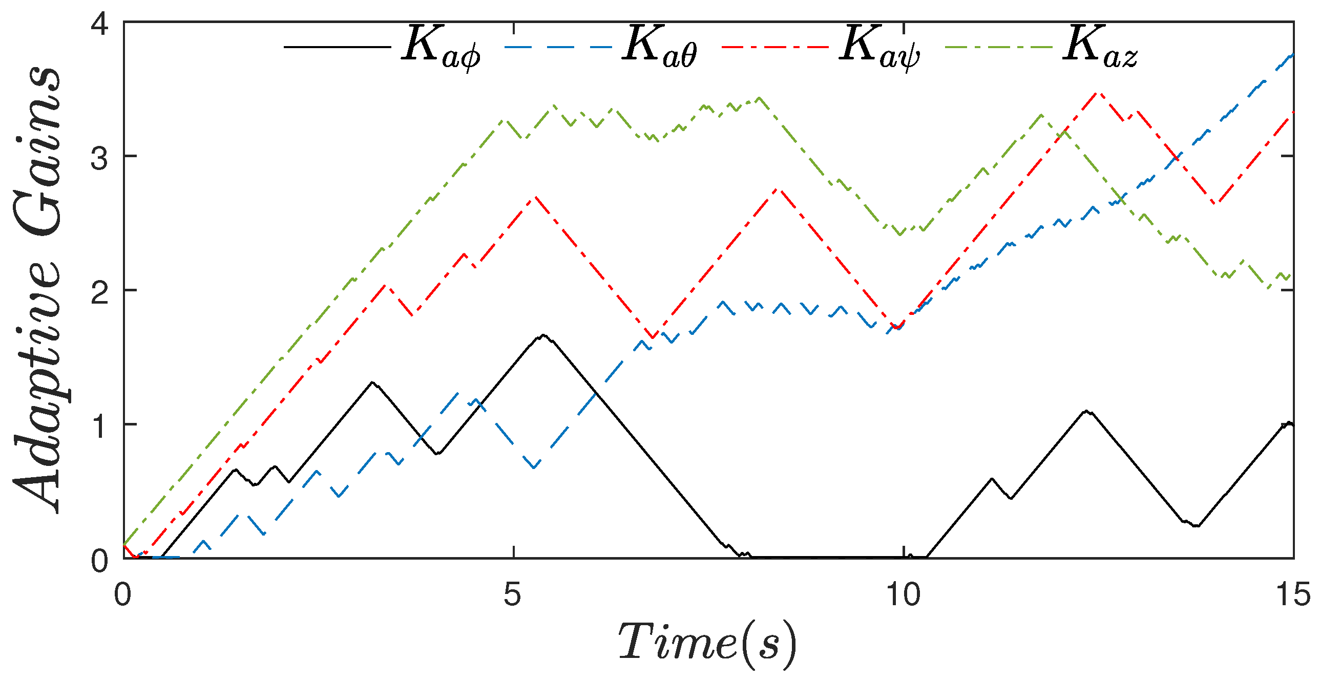
Figure 7 displays the evolution of the adaptive control gains. It is clear that at the start, the gains increased their values to reach the control objective, then they decreased until a defined minimal value, where stability was guaranteed.
4.2.2. Case with Perturbations
The second scenario considered model uncertainties, as well as external disturbances. Then, a perturbation, which consisted of a force induced by hand, was applied to the vehicle approximately in s. Recalling that this quadrotor MAV is tiny, external disturbances notably affect its performance. Figure 8 displays the state response, where the stabilization was clearly more difficult. Nevertheless, the adaptive flight control could achieve and keep stability even in the presence of such uncertainties and external perturbations.
Figure 9 shows the error response subject to external disturbances.
In Figure 10 as well, the corresponding angular velocities, which are the control inputs of the systems, are depicted. Again, due to its adaptive controller gains, the vehicle achieved and kept stability against uncertainties and external perturbations.
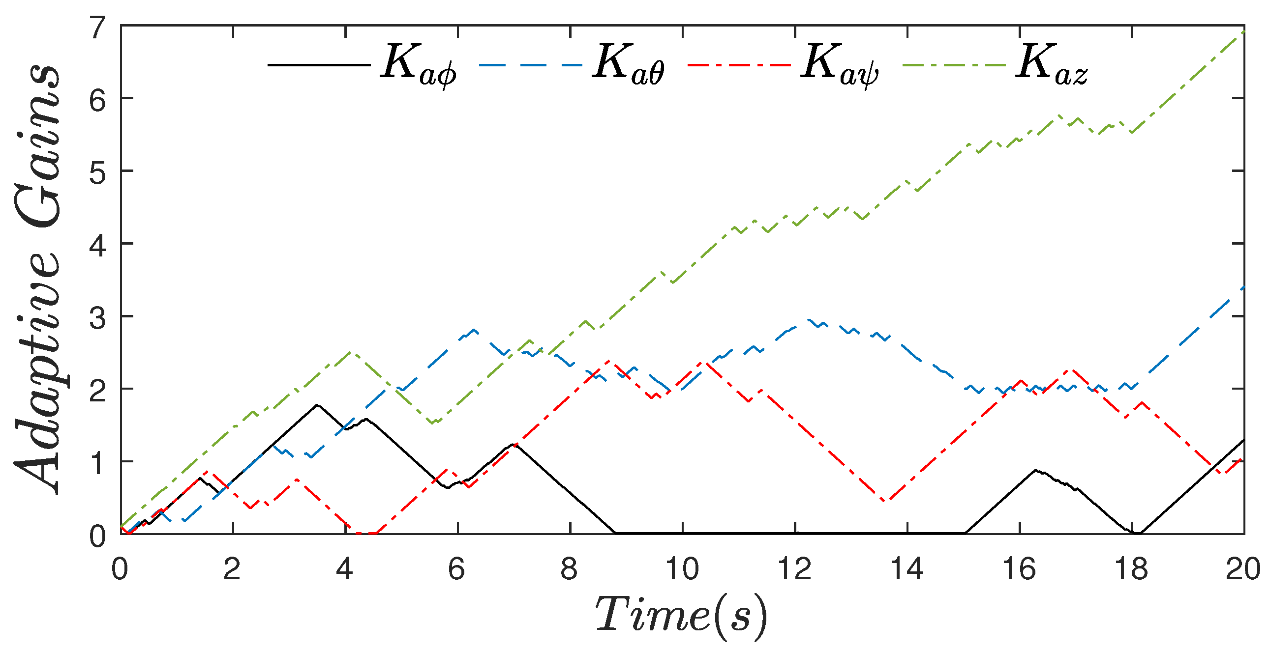
Finally, Figure 11 shows the adaptive control gains’ behavior under a perturbed environment; such a picture demonstrates that gains increase or decrease their values to reject such disturbances.
5. Conclusions
An embedded flight control for a quadrotor micro air vehicle subject to uncertainties and perturbations was designed and implemented. An adaptive sliding mode technique was the core of the approach, which was robust against bounded disturbances. Due to adaptive gains, necessary control was employed as the task requirement, reducing the chattering effect, and it was able to reject external perturbations. Even more, a stability analysis of the closed-loop system was provided. Finally, simulations and two experimental scenarios were conducted on a Parrot rolling spider micro drone, first with no perturbations and second disturbed, where the feasibility and advantages of the proposed control were demonstrated.
Author Contributions
Conceptualization, methodology, and formal analysis H.C.; supervision, J.L.G.
Funding
This research received no external funding.
Acknowledgments
The authors thank Sergio Lopez and Horacio Vorrath for their help in achieving the experiments and Laboratorio Nacional de Robotica del Centro y Norte de Mexico and Tecnologico de Monterrey for the facilities to carry out this research project.
Conflicts of Interest
The authors declare no conflict of interest.
Abbreviations
The following abbreviations are used in this manuscript:
| MAV | Micro Air Vehicle |
| UAV | Unmanned Aerial Vehicle |
| IMU | Inertial Measurement Unit |
References
- Cai, G.; Dias, J.; Seneviratne, L. Survey of Small-Scale Unmanned Aerial Vehicles: Recent Advances and Future Development Trends. Unmanned Syst. 2014, 2, 175–199. [Google Scholar] [CrossRef]
- Mathworks. Parrot Minidrones Support from Simulink. Available online: https://la.mathworks.com/hardware-support/parrot-minidrones.html (accessed on 14 June 2019).
- Available online: https://github.com/Parrot-Developers/RollingSpiderEdu (accessed on 14 June 2019).
- Dydek, Z.T.; Annaswamy, M.A.; Lavretsky, E. Adaptive Control of Quadrotor UAVs: A Design Trade Study With Flight Evaluations. IEEE Trans. Control Syst. Technol. 2013, 4, 1400–1406. [Google Scholar] [CrossRef]
- Mohd Basri, M.A.; Husain, A.R.; Danapalasingam, K.A. Enhanced Backstepping Controller Design with Application to Autonomous Quadrotor Unmanned Aerial Vehicle. J. Intell. Robot. Syst. 2015, 79, 295–321. [Google Scholar] [CrossRef]
- Satici, A.C.; Poonawala, H.; Spong, M.W. Robust Optimal Control of Quadrotor UAVs. IEEE Access 2013, 1, 79–93. [Google Scholar] [CrossRef]
- Gautam, D.; Ha, C. Control of a quadrotor using a smart self-tuning fuzzy PID controller. Int. J. Adv. Robot. Syst. 2013, 10, 1–9. [Google Scholar] [CrossRef]
- Guo, Y.; Jiang, B.; Zhang, Y. A novel robuts attitude control for quadrotor aircraft subject to actuator faults and wind gusts. IEEE/CAA J. Autom. Sin. 2018, 1, 292–300. [Google Scholar] [CrossRef]
- Xiong, J.; Zhang, G. Global fast dynamical terminal sliding mode control for a quadrotor UAV. ISA Trans. 2017, 66, 233–240. [Google Scholar] [CrossRef]
- Xiong, J.; Zheng, E. Position and attitude tracking control for a quadrotor UAV. ISA Trans. 2014, 53, 725–731. [Google Scholar] [CrossRef]
- Zheng, E.; Xiong, J.; Luo, J. Second order sliding mode control for a quadrotor UAV. ISA Trans. 2014, 53, 1350–1356. [Google Scholar] [CrossRef]
- Besnard, L.; Shtessel, Y.; Landrum, B. Quadrotor vehicle control via sliding mode controller driven by sliding mode disturbance observer. J. Frankl. Inst. 2012, 349, 658–684. [Google Scholar] [CrossRef]
- Luque-Vega, L.; Castillo-Toledo, B.; Loukianov, A. Robust block second order sliding mode control for a quadrotor. J. Frankl. Inst. 2012, 349, 719–739. [Google Scholar] [CrossRef]
- Rida, M.; Cherki, B. A new robust control for minirotorcraft unmanned aerial vehicles. ISA Trans. 2014, 56, 86–101. [Google Scholar] [CrossRef]
- Ramirez-Rodriguez, H.; Parra-Vega, V.; Sanchez-Orta, A.; Garcia-Salazar, O. Robust Backstepping Control Based on Integral Sliding Modes for Tracking of Quadrotors. J. Intell. Robot. Syst. 2014, 73, 51–66. [Google Scholar] [CrossRef]
- Sumantri, B.; Uchiyama, N.; Sano, S. Generalized super-twisting sliding mode control with a nonlinear sliding surface for robust and energy-efficient controller of a quad-rotor helicopter. Proc. Inst. Mech. Eng. Part C J. Mech. Eng. Sci. 2017, 231, 2042–2053. [Google Scholar] [CrossRef]
- Villanueva, A.; Castillo-Toledo, B.; Bayro-Corrochano, E.; Luque-Vega, L.; González-Jiménez, L.E. Multi-mode flight sliding mode control system for a Quadrotor. In Proceedings of the 2015 International Conference on Unmanned Aircraft Systems (ICUAS), Denver, CO, USA, 9–12 June 2015. [Google Scholar]
- Derafa, L.; Benallegue, A.; Fridman, L. Super twisting control algorithm for the attitude tracking of a four rotors UAV. J. Frankl. Inst. 2012, 349, 685–689. [Google Scholar] [CrossRef]
- Rajappa, S.; Masone, C.; Bulthoff, H.H.; Stegagno, P. Adaptive Super Twisting Controller for a Quadrotor UAV. In Proceedings of the IEEE International Conference on Robotics and Automation (ICRA), Stockholm, Sweden, 16–21 May 2016. [Google Scholar]
- Castañeda, H.; Gordillo, J.L. Spatial Modeling and Robust Flight Control Based on Adaptive Sliding Mode Approach for a Quadrotor MAV. Int. J. Intell. Robot. Syst. 2019, 93, 101–111. [Google Scholar] [CrossRef]
- Valavanis, K.P.; Vachtsevanos, G.V. Handbook of Unmanned Aerial Vehicles, 1st ed.; Springer: Dordrecht, The Netherlands, 2015. [Google Scholar]
- Haifeng, L. Multivariable Control of a Rolling Spider Drone. Master’s Thesis, University of Rhode Island, Kingston, RI, USA, 2017. Paper 1064. Available online: http://digitalcommons.uri.edu/theses/1064 (accessed on 14 June 2019).
Figure 1.
Referential frames’ configuration.
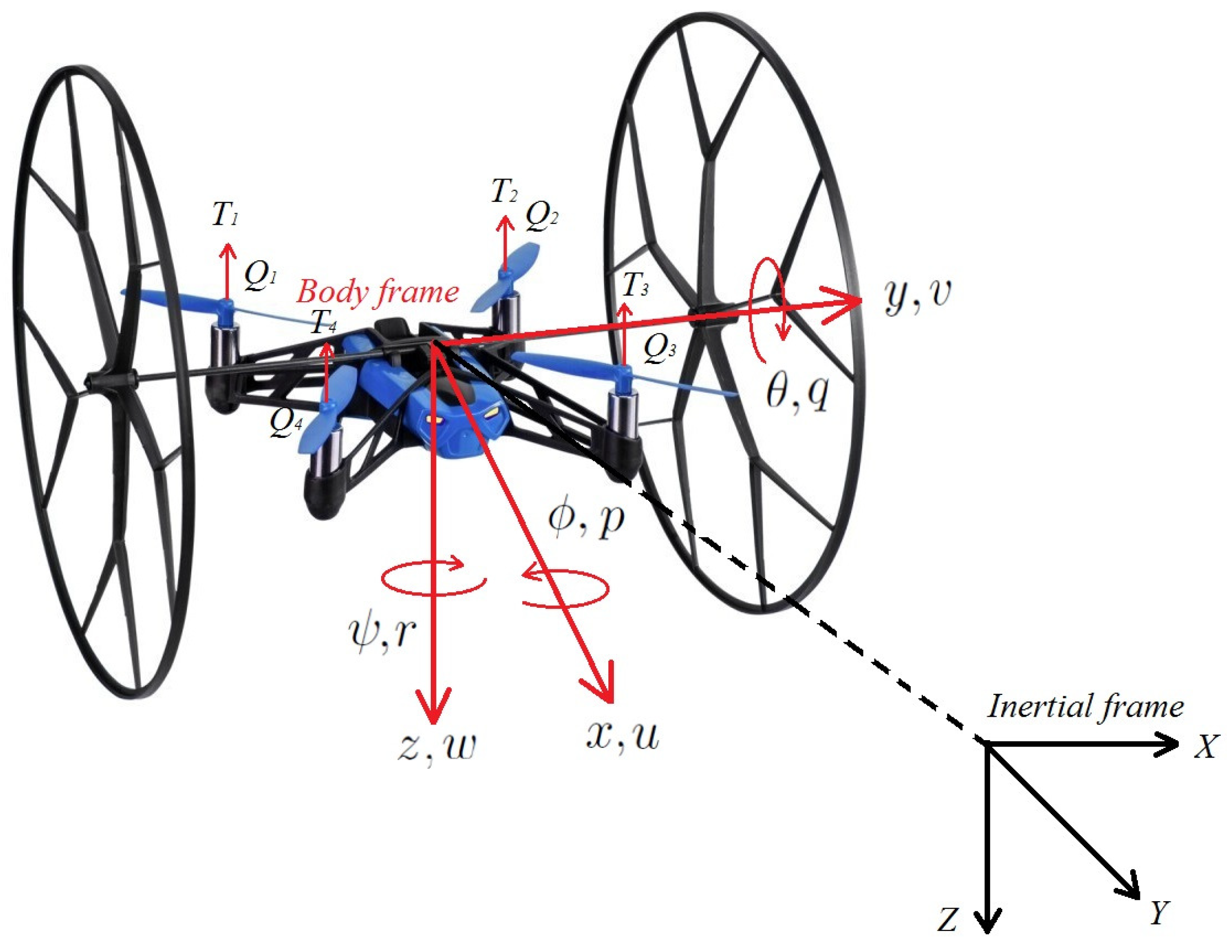
Figure 2.
Regulation. Controllers comparison: adaptive sliding mode control (asmc), feedback linearization (fbl), and proportional integral derivative with gravity compensation control (PID).
Figure 2.
Regulation. Controllers comparison: adaptive sliding mode control (asmc), feedback linearization (fbl), and proportional integral derivative with gravity compensation control (PID).
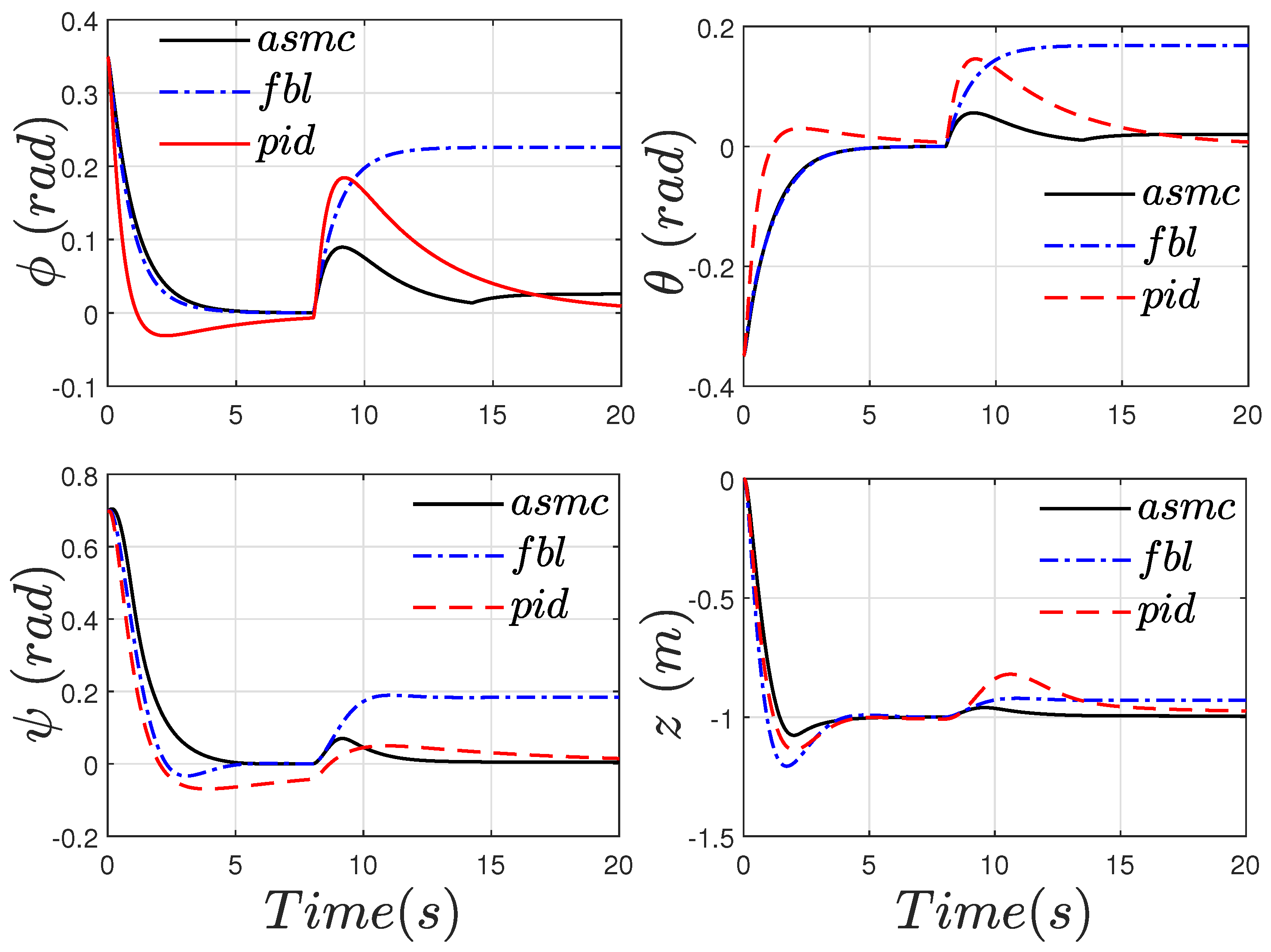
Figure 3.
Regulation. Control inputs of the controllers and adaptive gains of the asmc.
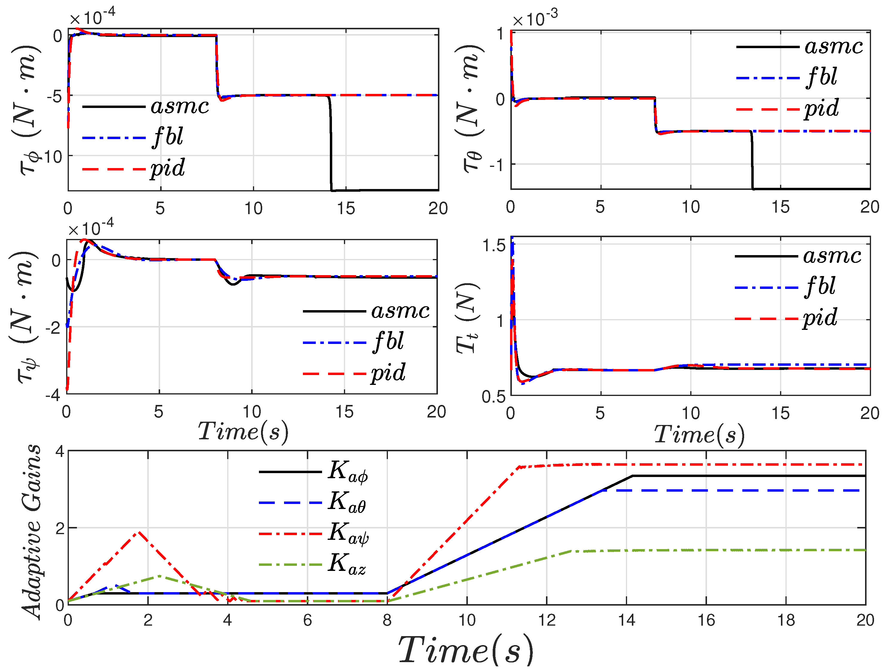
Figure 4.
Hovering. Pose of the quadrotor MAV.
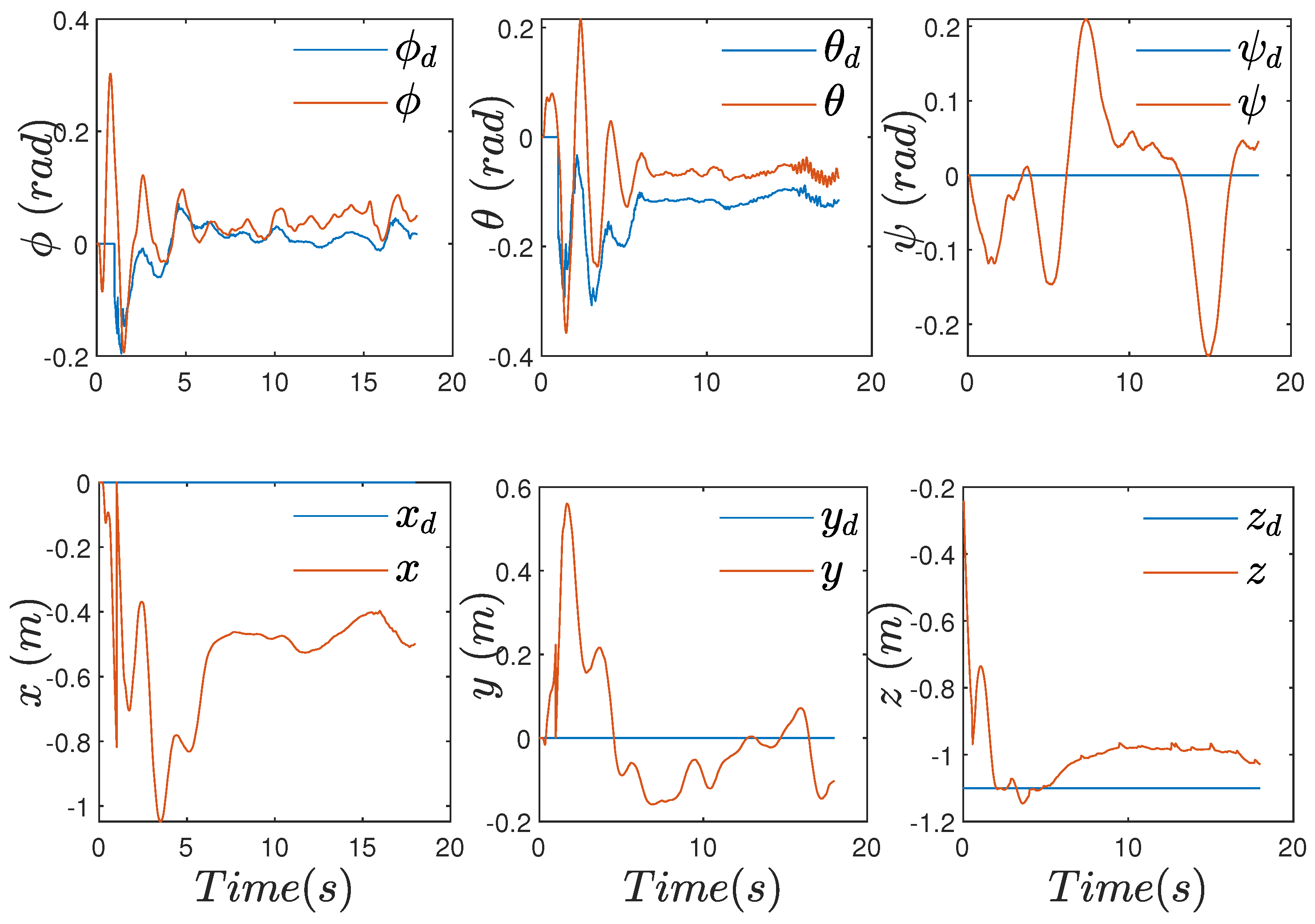
Figure 5.
Error, reference versus variable state.
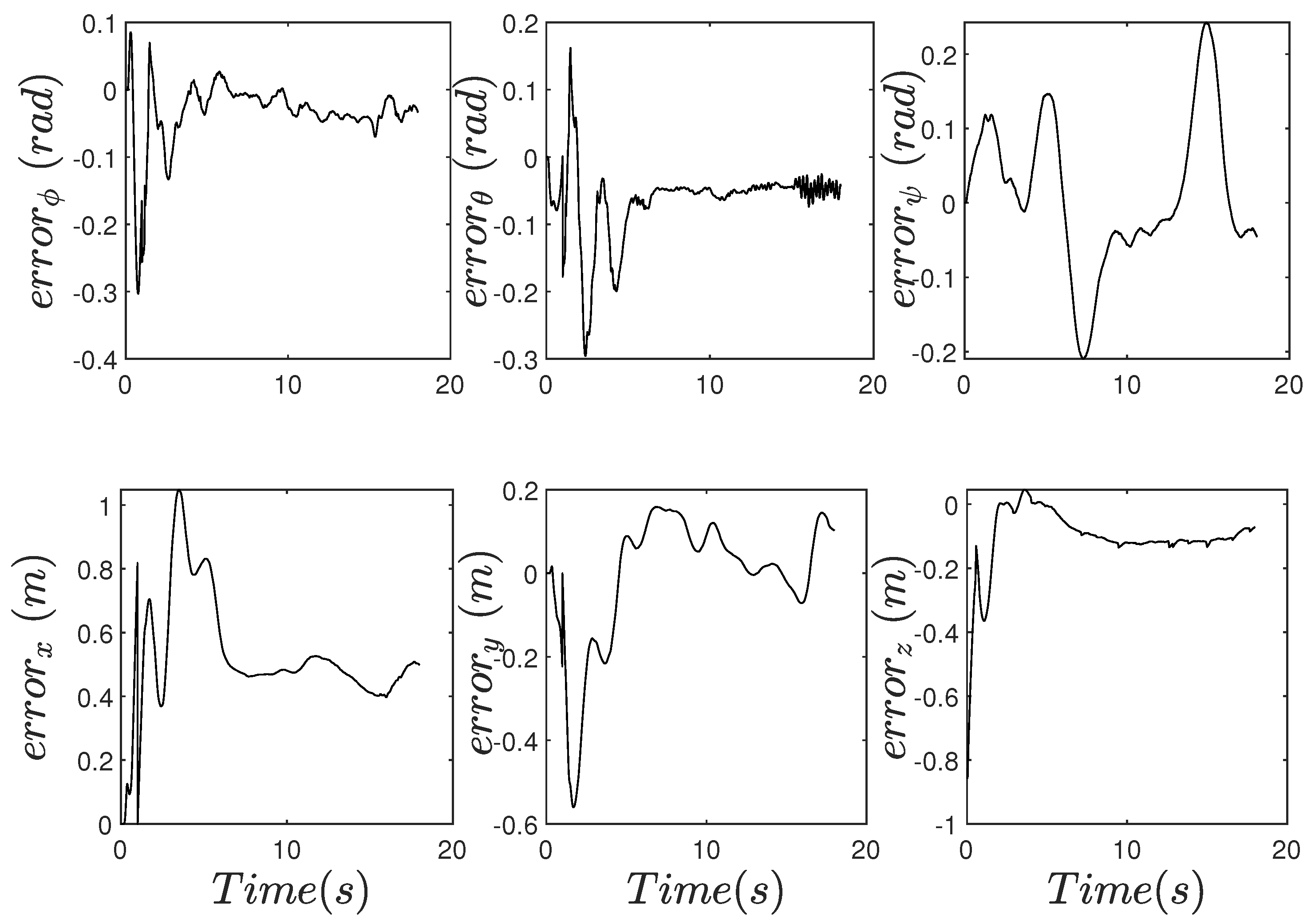
Figure 6.
Hovering. Control inputs of the quadrotor MAV.
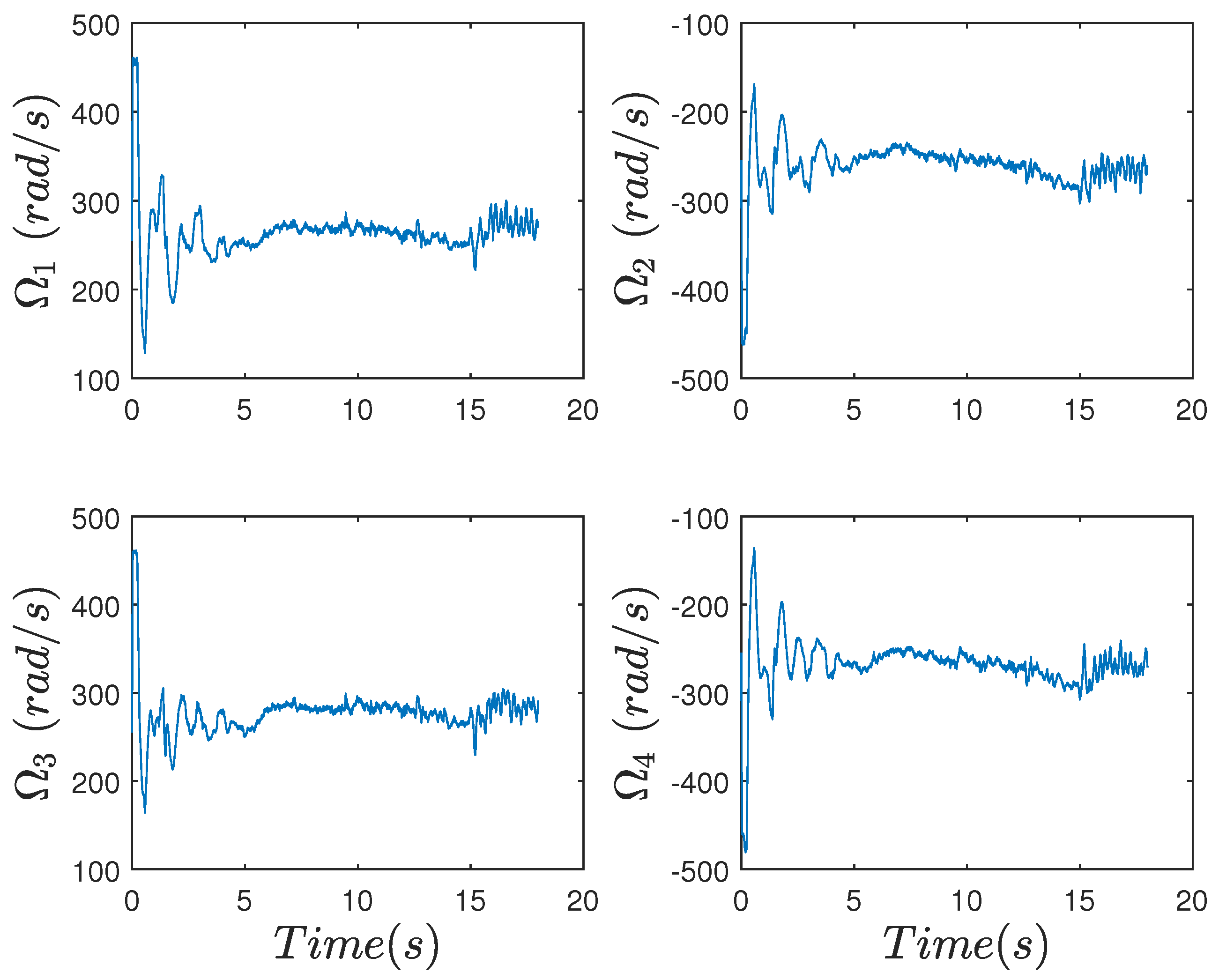
Figure 7.
Hovering. Adaptive control gains.

Figure 8.
Hovering. Pose of the quadrotor MAV subject to external perturbations.
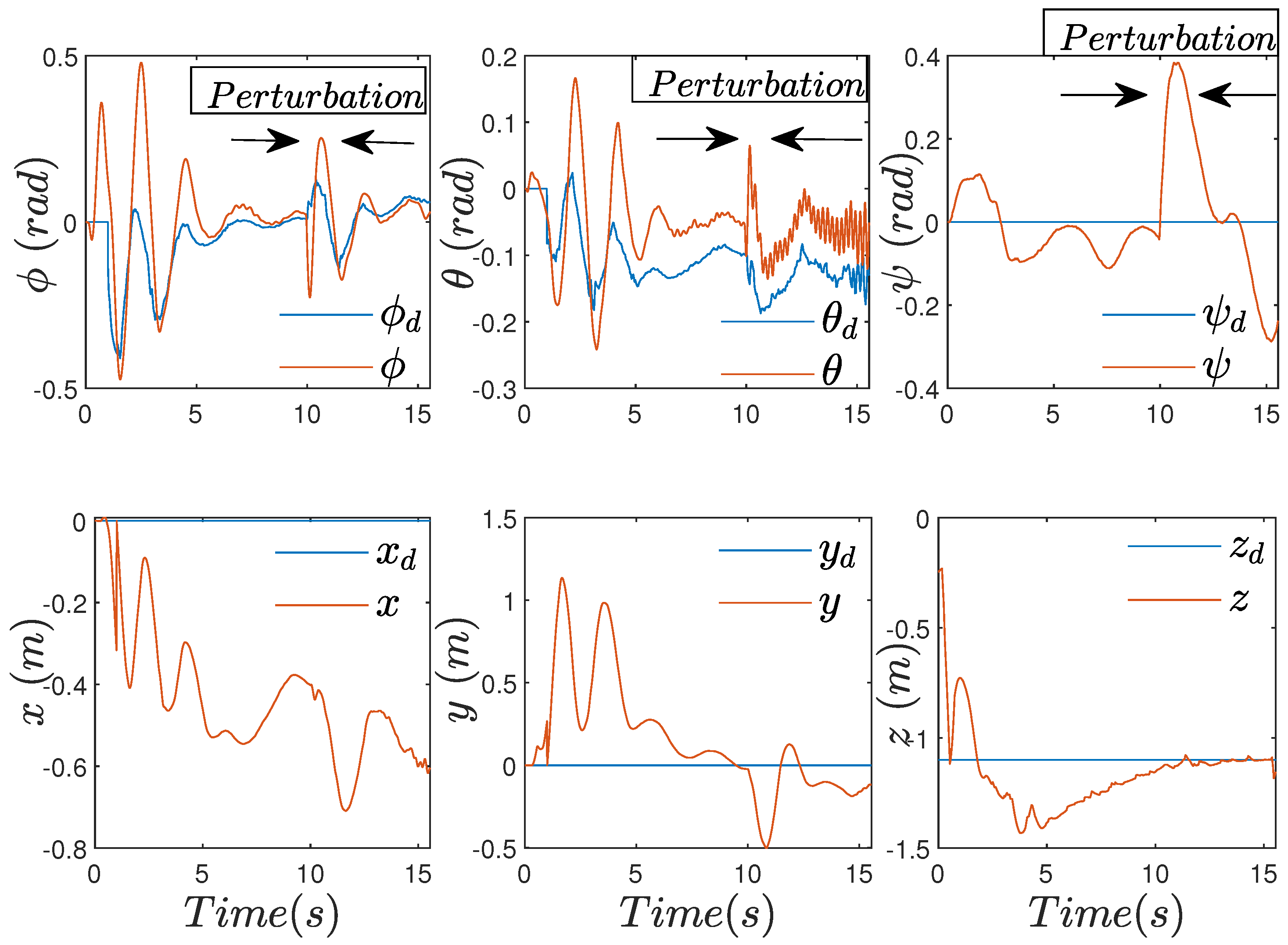
Figure 9.
Error. Reference versus variable state under perturbations.
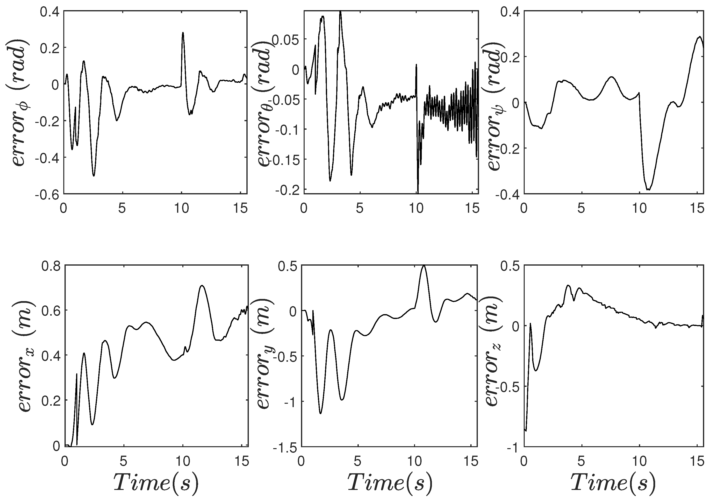
Figure 10.
Hovering. Control inputs of the quadrotor MAV under external perturbations.
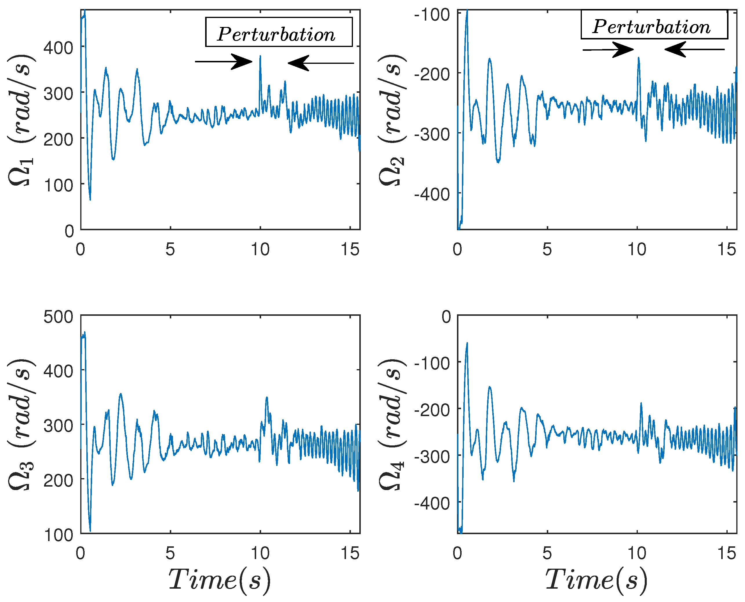
Figure 11.
Hovering. Adaptive control gains under external perturbations.

Table 1.
Quadrotor MAV model parameters [22].
Table 1.
Quadrotor MAV model parameters [22].
| Parameter | Value | Unit |
|---|---|---|
| Weight m | kg | |
| Arm length l | m | |
| Gravity g | m/s | |
| Inertia moment | kgm | |
| Inertia moment | kgm | |
| Inertia moment | kgm | |
| Thrust coefficient | N/(rad/s) | |
| Torque coefficient | Nm/(rad/s) |
© 2019 by the authors. Licensee MDPI, Basel, Switzerland. This article is an open access article distributed under the terms and conditions of the Creative Commons Attribution (CC BY) license (http://creativecommons.org/licenses/by/4.0/).
Share and Cite
MDPI and ACS Style
Castañeda, H.; Gordillo, J.L. Embedded Flight Control Based on Adaptive Sliding Mode Strategy for a Quadrotor Micro Air Vehicle. Electronics 2019, 8, 793. https://doi.org/10.3390/electronics8070793
AMA Style
Castañeda H, Gordillo JL. Embedded Flight Control Based on Adaptive Sliding Mode Strategy for a Quadrotor Micro Air Vehicle. Electronics. 2019; 8(7):793. https://doi.org/10.3390/electronics8070793
Chicago/Turabian StyleCastañeda, Herman, and J.L. Gordillo. 2019. "Embedded Flight Control Based on Adaptive Sliding Mode Strategy for a Quadrotor Micro Air Vehicle" Electronics 8, no. 7: 793. https://doi.org/10.3390/electronics8070793
Note that from the first issue of 2016, this journal uses article numbers instead of page numbers. See further details here.