A Survey on Deep Learning in Image Polarity Detection: Balancing Generalization Performances and Computational Costs

Abstract

Deep convolutional neural networks (CNNs) provide an effective tool to extract complex information from images. In the area of image polarity detection, CNNs are customarily utilized in combination with transfer learning techniques to tackle a major problem: the unavailability of large sets of labeled data. Thus, polarity predictors in general exploit a pre-trained CNN as the feature extractor that in turn feeds a classification unit. While the latter unit is trained from scratch, the pre-trained CNN is subject to fine-tuning. As a result, the specific CNN architecture employed as the feature extractor strongly affects the overall performance of the model. This paper analyses state-of-the-art literature on image polarity detection and identifies the most reliable CNN architectures. Moreover, the paper provides an experimental protocol that should allow assessing the role played by the baseline architecture in the polarity detection task. Performance is evaluated in terms of both generalization abilities and computational complexity. The latter attribute becomes critical as polarity predictors, in the era of social networks, might need to be updated within hours or even minutes. In this regard, the paper gives practical hints on the advantages and disadvantages of the examined architectures both in terms of generalization and computational cost.

1. Introduction

“A picture is worth a thousand words” is an English idiom that is becoming every day more actual. Mainly thanks to social networks, images have become one of the most important communication tools in the world. Every day, users share millions of images and videos; in most of the cases, this content is expected to convey affective information. As a result, sentiment analysis is recently witnessing an increasing number of applications to multimedia resources [1,2,3], in addition to text-only resources [4,5,6,7,8,9,10].

Sentiment analysis is a branch of data mining that aims to aggregate emotions and feelings from different types of documents. Image polarity detection indeed addresses a specific task within this framework: to distinguish images that raise positive emotions in human users from images that cause bad sentiments [11,12,13,14]. Image polarity detection stimulates interest both from industry and academia, as its applications are countless [15], e.g., human–robot interaction, stock market prediction, political forecasting, and social network analysis. In fact, in recent years, several works addressed this relatively new topic [1,2,16,17].

The literature highlights the advantages of deep learning in applying sentiment analysis to images. Deep networks can yield powerful tools for automating the process of feature extraction, which may prove challenging when dealing with complex, two-dimensional sources of information such as images. The ability of deep networks to support automated feature extraction stems from a new approach to learning, which disregards the traditional division between feature learning and classifier learning. Accordingly, the training process is designed to learn both the classification rule and a meaningful representation of the input patterns. Hence, deep networks play a major role in all the areas where the learning problem involves complex and stratified feature sets [18]; for example: healthcare [19], time series analysis [20], and object detection [21]. In the case of polarity detection, deep networks can accomplish the task of understanding the interaction between the different components of an image. Moreover, they can effectively support object recognition, which is a prerequisite to characterizing the interactions between objects.

Polarity, however, also depends on the context in which the image is examined, as the same objects, and even the same images, can lead to different polarities in different scenarios. Figure 1 is a clear example of a picture that can be interpreted otherwise, depending on both cultural background and historical moment: in the past, rainbow flags were associated with pacifist movements, whereas currently, they mostly relate to homosexual rights. As a result, in the current era of social media, content marketing, and custom profiles, a thorough re-training of the polarity-detection strategy might be required within a short time interval (even minutes or hours) to keep the pace of evolving circumstances. Re-training a deep network, however, raises major issues when addressing image polarity: firstly, one cannot take the availability of many labeled data for granted; secondly, the complexity of the learning process might require massive computational resources to support fast training.

The paradigm of transfer learning [23,24,25] can provide a viable solution to both issues. According to its general definition, in transfer learning, one reuses an existing model (optimized for a given task) as a starting point to develop an upgraded model, for a somehow related task. In practice, transfer learning involves a wide range of approaches [24,25], which are designed to cover a variety of scenarios. The most important aspects in these cases are the amount of labeled data, the expected similarity between the source domain and the target domain, and the characteristics of the specific optimization problem. On the other hand, the great majority of the literature related to image polarity detection relies on a specific scenario. A deep network trained for object recognition provides the starting point, mostly because in that case, a huge amount of labeled data is accessible and one can benefit from a consistent number of effective trained models. By contrast, the target domain of polarity detection can only provide a limited amount of labeled samples.

The literature confirms that transfer learning can yield superior performances in image polarity detection [1,2,16]. Some crucial issues, however, remain open: first, to the best of the authors’ knowledge, a fair, comprehensive comparison is lacking between the various approaches to image polarity detection when starting from object recognition. In the latter case, the predictors are usually built around convolutional neural networks (CNN) that support the feature-extraction process for object recognition, but the choice of the specific CNN adopted is indeed critical, as the literature offers in turn a variety of options. This eventually leads to the second open issue, which relates to the run-time performance: adopting a specific CNN ultimately affects the generalization ability of the eventual predictor, its training time, and the computational cost of the inference phase. In this sense, little attention has been given in the past to the trade-off between the computational costs and generalization abilities.

Contribution

The proposed research yields a two-fold contribution. First, the paper presents a careful analysis of the cutting-edge technologies for image polarity detection. The paper reviews (1) all the relevant CNN architectures for object recognition and (2) the most effective approaches to image polarity detection based on CNNs.

Secondly, the paper introduces an experiment-design strategy to attain a fair comparison between different configurations of image-polarity detectors. The proposed benchmark involves three different configurations and implementations of the transfer-learning process. The alternatives satisfy the constraints imposed by a realistic scenario: (1) a limited amount of images with polarity labels is available, and (2) the training process can only rely on limited computational resources. The comparison involved eight different CNNs for object detection, and the eventual predictors were evaluated according to three attributes: classification accuracy, the computational cost of the training process, and the computational cost of the inference phase. Four real-world established datasets formed the benchmark for the experimental evaluation. As a result, this work provides a handbook for the selection of the right architecture, according to the available computational resources and the expected generalization performances.

The rest of the paper is organized as follow. Section 2 provides a brief overview of the various architectures adopted for object recognition. Section 3 analyzes the literature and reports on the several design approaches for implementing image-polarity detection via transfer learning. Section 4 defines the design of the experiment that was used to discriminate the contributions of the CNNs in the associated polarity-detection frameworks. Section 5 characterizes the three configurations in terms of the computational complexity of the training process. In Section 6, the outcomes of the experimental sessions involving the benchmarks are presented and discussed. Finally, Section 7 makes a few concluding remarks.

2. CNNs for Object Recognition

This section briefly reviews the most significant CNN architectures, especially for object recognition, which have already been used in the development of frameworks addressing image polarity detection.

The AlexNet [26] deep network first achieved important results in the field of image classification. In its standard configuration, that architecture included eight weight layers (five convolutional layers and three fully = connected layers). Overall, AlexNet was characterized by $61·{10}^6$ parameters. This feature clearly raised a major issue in terms of computational load, since the classification performance strictly depended on the availability of huge training sets. This problem was suitably tackled thanks to the computational power of graphics processing units (GPUs). GPUs proved decisive to tackle the trade-off between training time and the size of the training set. That research actually opened the way to the massive use of GPUs for the computational support of deep learning.

Vgg_16 and Vgg_19 [27] improved the architecture of AlexNet by increasing the number of weight layers to 16 and 19, respectively; besides, these architecture exploited exclusively stacks of $3\times 3$ convolutions. Both Vgg_16 and Vgg_19 proved able to outperform AlexNet in terms of classification performance. On the other hand, they also inflated the number of parameters to be set by the learning process.

In 2014, GoogLeNet [28] introduced major novelties in the design of CNN architectures by proposing the Inception Module. Such a module implements a local, small network topology as shown in Figure 2. First, the output of the previous layer feeds different filter operations, which are completed in parallel. Then, the outcomes of the filters merge into one third-order tensor, thus projecting the resulting depth to a lower dimension. This strategy allows the eventual stack of Inception Modules to limit the amount of parameters involved. In its standard configuration, GoogLeNet featured 22 weight layers and still involved less parameters than AlexNet. Indeed, this architecture has been progressively updated (e.g., Inc_V3 [29], and Inc_v4 [30]).

ResNet architectures [31] tackled the design of very deep networks by using Residual Net as building blocks, which replaced standard convolutional modules. A Residual Net is entitled to fit $\mathit{F}\left(\mathbf{x}\right)=\mathit{H}\left(\mathbf{x}\right)-\mathbf{x}$, where $\mathit{H}\left(\mathbf{x}\right)$ is any desired mapping (under the assumption that $\mathit{H}\left(\mathbf{x}\right)$ and $\mathbf{x}$ have the same dimensionality). Overall, the architecture is organized as a stack of such blocks, in which each element is trained on the residual representation of the previous one. Thus, in the lth layer, one has:

$${\mathbf{x}}_l={\mathit{F}}_l\left({\mathbf{x}}_{l-1}\right)+{\mathbf{x}}_{l-1}.$$

(1)

Figure 3 outlines the overall structure of a Residual Net. This architecture aims to deal with the convergence issues brought about by the complexity of deep networks. Res_50, Res_101, and Res_152 adopted, respectively, a total of 50, 101, and 152 weight layers.

Finally, the DenseNet architecture [32] introduced a different approach: each layer was connected to every other layer in a feed-forward fashion. Basically, the eventual architecture was organized as a stack of Dense Blocks; in the $l$ layer, one has:

$${\mathbf{x}}_l={\mathit{F}}_l\left([{\mathbf{x}}_0,{\mathbf{x}}_1,\dots ,{\mathbf{x}}_{l-1}]\right),$$

(2)

where $[{\mathbf{x}}_0,{\mathbf{x}}_1,\dots ,{\mathbf{x}}_{l-1}]$ is the concatenation of the outputs of the previous layers. The overall layout was designed to achieve two goals: (1) to strengthen feature propagation and (2) to reduce the total number of parameters. Different configurations of the DenseNet architecture were proposed in [32]. DenseNet-BC proved to be the most effective at dealing with the ImageNet benchmark [33].

Table 1. Attributes of different CNN architectures exploited in the area of object recognition.

Architecture	Weight Layers	Acc (%)	Operations (Gflops)	Parameters ($\times {10}^6$)
AlexNet [26]	8	54	$\mathbf{0.7}$	61
Vgg_16 [27]	16	71	15.5	138
Vgg_19 [27]	19	71	19.6	144
GoogLeNet [28]	58	68	1.6	$\mathbf{7}$
Inc_v3 [29]	46	78	6	24
Res_50 [31]	50	76	3.9	26
Res_101 [31]	101	77	7.6	45
Res_152 [31]	152	79	11.3	60
DenseNet [32]	201	77	4.0	20

gives the main details of the architectures discussed above. For each network, the table provides: the number of weight layers, the classification percentage accuracy scored in the ImageNet [33] competition, the number of floating point operations required by one image classification [34], and the total amount of parameters. The number of parameters mostly affects memory occupation and the required size of the training set. When using a pre-trained network as the starting point, transfer learning can require a smaller number of samples to attain fine-tuning successfully. On the other hand, the size of the training set strictly relates to the number of parameters. The number of floating point operations reasonably reflects the computational complexity of the architecture. In fact, a detailed metric should take into account the fact that, in general, different instructions have different computational costs (e.g., memory access timings), and this therefore affects computational performance. The table shows that GoogLeNet seems the best choice in terms of both parameters and computational complexity, whereas the other comparisons (except for AlexNet) outperformed GoogLeNet in terms of accuracy.

3. Image Sentiment Analysis: State-of-the-Art

Image polarity detection is an emerging topic in the area of sentiment analysis and has been covered recently by interesting surveys [1,2,16,17]. With respect to those works, this paper focuses instead on the role played by CNN architectures and transfer learning in that domain. Several relevant papers addressed the image polarity-detection problem before the spread of deep learning for image processing [22,35,36,37,38,39,40,41,42,43], and the approaches based on CNNs today represent the state-of-the-art in this area.

3.1. Polarity Detection

Approaches to polarity detection usually reflect the basic structure of object recognition frameworks. In compliance with the transfer learning paradigm, subjectivity detection relies on lower-level features that are worked out by a CNN, optimized for object recognition. In practice, this approach leads to two design alternatives, as outlined in Figure 4.

In Figure 4a, access to low-level features is attained by removing the topmost (fully-connected) layer of the pre-trained CNN. The features either feed a new fully-connected layer, including as many neurons as the classes involved in the polarity detection problem, or an ad-hoc classifier. A fine-tuning process allows re-training the CNN to adjust both its parameters and the resulting features according to the specific polarity-detection problem.

In the second approach as per Figure 4b, the eventual classifier stems from a two-step procedure: first, the topmost fully-connected layer in the trained CNN is replaced with a new architecture that models an ontology. The resulting layout is re-trained by using a visual sentiment ontology (VSO). Several approaches relied on adjective-noun pairs (ANPs) [11,12], which provide a collection of images for a given pair {adjective, noun}. In the second step, the new layout becomes the building block of the polarity detector. Therefore, as done in the first design approach, one might disconnect the topmost fully-connected layer and get access to the features. Otherwise, one might plug a specific classifier on top of the layout; in this case, the input values to this classifier would follow the probability distribution of the classes characterizing the underlying ontology. A final training process then configures the additional, topmost layout. In general, the learning process in the first step is affected by weak labels, since VSOs are worked out by automated algorithms that add some noise to the labeling result.

Notably, in the first design, the assumption was that mid-level features can be inherently extracted by the CNN. Differently, the second design explicitly models the mid-level features by using an ontology. In principle, the first design tackles a more challenging problem; on the other hand, good local minima can be reached also with a modest amount of training data. The second design conversely requires a huge training set because an ontology involves several classes.

The literature offers a variety of implementations of both design strategies. The implementations mostly differ in the adopted CNN, in the transfer-learning methodology, and the specific domain from which the training data are drawn. A few papers relied on AlexNet for low-level feature extraction in the schema as per Figure 4a. In [11], a logistic regression layer supported the classifier, and the comparison covered two approaches: (1) the classifier replaced the topmost fully-connected layer in AlexNet; (2) the classifier was stacked over the AlexNet architecture. Campos et al. [44] adopted AlexNet as a feature extractor and yielded an interesting analysis on the effects of both layer ablation and layer addition on the accuracy performance of polarity detection. A design based on ontology representation (as per Figure 4b) was adopted in [45]; the authors developed a sentiment-recognition layout based on AlexNet, in which the topmost layer included one neuron for each ANP. This approach outperformed the SentiBankclassifier based on SVMs [22] and was employed for egocentric sentiment prediction in [46]. Jou et al. [47] improved on the approach presented in [45] by a multilingual visual sentiment ontology (MVSO). The methodology presented in [12] involved a custom architecture for image polarity prediction: the model included a pair of convolutional layers and four fully-connected layers. The training procedure involved weak labels generated by ANP. The authors followed a multi-step learning strategy: after each step, the dataset was pruned by taking out the images that had been classified correctly. A comparison between this approach, the architectures discussed in [44], and the method proposed in [47] was presented in [14], in which the authors focused on the role played by the specific ontology in transfer learning. The best performances were scored by the models relying on AlexNet and on the English version of MVSO. The Vgg_19 and the GoogLeNet architectures were implemented in [13,48], respectively. Interestingly, the papers pointed out that the predictors based on the compared architectures outperformed state-of-the-art predictors based on AlexNet. In [49], the authors compared Vgg_16, Res_50, Inc_v3, and the approach presented in [12] for outdoor polarity detection and proved that the model proposed in [12] compared favorably with the other three alternatives. In addition, the paper showed that higher accuracy performances could be obtained by combining the four CNNs in an ensemble.

The enhancement of the ontology representation in the schema of Figure 4b was the specific goal of some works. Fernandez et al. [50] proposed a framework in which two independent CNNs were adopted to learn ANPs, one network to deal with nouns and the other to deal with adjectives. Both predictors relied on the Res_50 architecture. A similar approach was used in [51], but the eventual framework followed a different strategy to merge the information provided by the two CNNs. Wang et al. [52] proposed a model in which adjectives and nouns were predicted by different CNNs; the two networks were coupled by a mutual supervision mechanism. A modified version of Res_50 supported the model proposed in [53]; in that case, the residual learning mechanism was extended to multitask cross-residual learning. As a result, a single network could manage explicitly the interactions between different ANP couples (e.g., “shiny-cars”, “shiny-shoes”).

CNN architectures also supported models for image polarity detection that did not fit into either of the two designs schemes described above. In [48], the Vgg_19 architecture processed an image including the conventional R, G, and B channels and a focal channel; the latter channel was set to model human attention. Likewise, the works in [54,55] studied the relevance of salience in sentiment detection. Attention mechanisms [56,57] were addressed in [58], where the authors combined VggNet architectures with a recurrent neural network (RNN). The RNN allowed the model to explore an image as a composition of small areas, thus mimicking the human attention process in which a person only focuses on significant areas of the image. The approach based on the exploration of small regions further evolved to [59,60], which introduced two approaches explicitly designed to learn salient regions of an image. Those models integrated Vgg_16 and ResNet_101 into ad-hoc architectures that combined polarity detection with the local information embedded in images. In the paper by Rao et al. [61], a fast R-CNN located the distinctive parts of an image. The approach by Song et al. [62] combined attention and salience. The procedure extracted a pair of maps for salience and attention from an input image and worked out a score based on the correspondence between the pair. The system was completed by a VggNet for extracting features. In [63], the authors combined VggNet with art features to enhance the model effectiveness at finding the image polarity. In [64], the same CNN structure computed features in an integrated framework, which embedded low-rank and inverse-covariance regularization terms to learn a robust feature representation and a reasonable prediction model at the same time. Finally, Balouchian et al. [65] explored the use of context information to enhance VGGNet_16 and Res_50.

Table 2. Usage of object detection architectures in the reviewed papers.

Architecture	Schema
	Standard	Ontology	Ad-hoc
AlexNet	[11,44]	[45,46,47]	-
Vgg	[48,49]	[51]	[48,54,55,58,59,62,63,64,65]
Inception	[13,49]	-	-
ResNet	[49]	[50,53]	[60,65]
Custom	[12,49]	[52]	-

summarizes the various options for object detection architectures within image-polarity frameworks. The table rows group the object-detection architectures into families; for example, the ResNet entry indexes all the networks characterized by residual layers. The table columns refer to the various approaches for image polarity detection. The column marked as “Standard” identifies all those approaches that can be summarized according to the schema illustrated in Figure 4a. Likewise, the third column (“Ontology”) indexes models that follow the design in Figure 4b. The last column (“Ad-hoc”) identifies models that do not fit the previous categories.

3.2. Sentiment Analysis: Other Applications

The automated generation of image captions with sentiment terms is closely related to sentiment prediction and aims to extract affective information from images. Actually, a crucial aspect concerns how information is conveyed, since the final user of a caption-generation model is a person. The archetypal model [66] in this field included a CNN architecture that fed gated RNNs [67]. The CNN extracted low-level features from the image, while a long short-term memory (LSTM) network modeled the textual description of the image. In [68,69,70], a VggNet architecture was adopted to extract low-level features; in [71], such a task was accomplished by a Res_152 architecture. Karayil et al. [72], conversely, used AlexNet to model ANPs; a multi-directed graph ranked the ANP couples provided by the CNN and generated captions accordingly. For the purpose of improving sentiment description, Sun et al. [73] extended a pre-trained caption generation model with an emotion classifier to add abstract knowledge.

Image polarity detection can also apply to multimodal sentiment analysis. Remarkable results have been achieved in [74,75,76,77,78,79], where ensembles of handcrafted features were worked out from images and combined with information provided by text analysis. Those approaches were subsequently outperformed by frameworks that integrated CNNs for extracting features from visual content [12,78,80,81,82,83,84,85].

In addition to polarity-based methods, fine-grained representations of sentiments were addressed in [52,86,87,88,89,90,91,92]; approaches ranged from multi-class labeling to continuous probability distributions. The common rationale is that one image can evoke several feelings at the same time. Both analogical and discrete models were employed to describe the emotional contents of the images. From a methodological view point, though, that research did not convey any significant novelty about the automated feature extraction process via CNNs, since most of them relied on ensembles of handcrafted features, with the partial exception of [89,90]. In [89], the authors introduced a custom architecture, including three convolutional layers and three fully-connected layers. That structure for polarity detection contributed to a framework for the classification of emotional states into eight categories. The final prediction of the polarity model introduced a bias in the final result, by activating a subset of neurons of a fully-connected layer that prompted the eventual prediction. Zhao et al. presented in [90] an ensemble of features composed of handcrafted features and the representation retrieved using the AlexNet architecture. Recently, ref. [93] embedded a ResNet architecture within a domain-adaptation framework.

It is worth mentioning, finally, that polarity and sentiment detection were also exploited in face analysis [94,95,96,97,98,99], posture analysis [100], brain signals [101], and the behavioral analysis of groups of people [102]. These methodologies were tailored to specific tasks and strictly related to the video domain.

3.3. Benchmarks

Table 3. Benchmarks for image sentiment prediction. ANP, adjective-noun pair; MVSO, multilingual visual sentiment ontology.

Name	Size	Classes	Supplementary Material
Twitter [12]	882	2	n.a.
Phototweet [22]	603	2	text
Multi-view [74]	19,600	3	text
OutdoorSent [49]	1950	3	n.a.
Flickr [76]	105,587	2	text
Instagram [76]	120,000	2	text
IAPS [103]	394	8	n.a.
Art photo [37]	807	8	n.a.
Abstract paintings [37]	228	8	n.a.
Image-Emotion-Social-Net [92]	1,434,080	8,2, continuous	n.a.
MVSA [104]	23,308	8	n.a.
Twitter_LDL [87]	10,045	8	n.a.
T4sa [105]	1.5 M	3	text
Flickr_LDL [87]	10,700	8	n.a.
Visual Realism [48]	2520	2	n.a
LUCFER [106]	3.6 M	275	context
ANP [22]	1 M	23,244	adjective name pairs
MVSO(EN) [47]	4 M	4422	adjective name pairs

lists the most common benchmarks in the area of image sentiment prediction. The table intentionally does not include datasets designed for caption generation, face-sentiment detection, and multimodal analysis. The first column marks the name of the dataset with the reference paper; the second and third columns give the size of the dataset and the number of classes, respectively; the last column lists possible supplementary material provided with the images.

All the benchmarks involving two classes explicitly referred to polarity detection. The datasets Multi-view, T4sa, and OutdoorSent can be viewed as special cases, as they also included the class neutral. Except for Twitter and OutdoorSent, the benchmarks also provided the textual message associated with each image. The benchmarks involving eight classes, instead, referred to emotion recognition. LUCFERincludes a large collection of images with contextual information; the labels were obtained by merging sentiment and context information. The last pair of datasets in Table 3 are examples of ontologies, which associated a collection of images with the corresponding adjective-noun pairs. Such datasets can support the design implementation illustrated in Figure 4b. The ANP dataset also provided the polarity of single ANPs pairs. Finally, in [92], the authors introduced a dataset that provided three kinds of labels for each pattern, thus allowing multiple analysis of the dataset.

4. A Comparative Analysis

A crucial result of the literature reviewed in the previous section is that CNNs are widely used for feature extraction (in the transfer-learning setup) in all the frameworks that need to rely on image sentiment analysis. The various design approaches differed in terms of both the feature extraction process and the overall polarity predictor arrangement. Thus, one deals with a plethora of heterogeneous approaches, which may be classified according to the adopted pre-trained CNN, the training dataset, and the fine-tuning strategies. Such a variety makes it difficult to evaluate the actual contribution yielded by a given setup in boosting the performance of image polarity detection.

This paper aims to address this issue by proposing a formal experimental protocol, to support a fair comparison between different configurations of polarity predictors and different setups of feature extractors. In this sense, the schema introduced in Figure 4a is used as a reference, mostly because it covers three general, distinct configurations, as shown in Figure 5. Such configurations differ in the classification block that processes the outputs of the pre-trained CNN and in the learning strategy applied to the resulting predictor; the latter option may either include or not a fine-tuning procedure for the parameters of the pre-trained architecture. In the figure, bold identifies blocks that are trained from scratch for polarity detection, whereas italics identify pre-trained blocks that are just subject to fine-tuning. These configurations cover the majority of the setups proposed in the literature for image polarity detection. Moreover, they satisfy the (reasonable) constraints taken into account in the proposed analysis, i.e., (1) a small number of images with polarity labels is only available for fine-tuning, and (2) the computational resources are limited. The details of the three configurations will be discussed in Section 4.1, Section 4.2 and Section 4.3, respectively.

The configurations illustrated in Figure 5 can highlight the specific contributions of the CNN architectures to the overall prediction performances. In this regard, the present analysis covered two main aspects: the accuracy of the predictor and the computational load brought about by the associated learning process. In contrast, it would seem that the configurations following the design strategy as per Figure 4b would prove less effective to support a fair comparison between the possible alternatives. This is because the intermediate layers, deployed to model ontologies, might actually introduce some bias, due to both the actual configuration of those layers and the adopted ANP. The latter aspect is indeed critical because ontologies tend to induce a cultural bias [47,107], as well. The tested configurations could benefit from an unbiased background, by only relying on CNNs that had been pre-trained with the ImageNet dataset [33], which gave a well-established benchmark in object-recognition applications.

4.1. Layer Replacement

The configuration outlined in Figure 5a refers to the most common layout for image polarity detection: the topmost fully-connected layer of a CNN that has been previously trained on object recognition is replaced with a new fully-connected layer. The latter layer includes as many neurons as the number of classes in the polarity problem and acts as a classification layer for the eventual prediction outcome. The eventual predictor system performs as a universal approximator, which integrates a feature-extraction block (whose parameterization is inherited from object recognition) and a classification layer (which has to be trained from scratch). This approach allows training the predictor on the new application domain in a limited number of epochs. When extending training to the feature extraction block, one implements fine-tuning, but by suitably setting the learning rate, the adjusted parameters therein are only subject to small perturbations [23].

Similar configurations can be obtained by implementing other strategies of layer ablation. Campos et al. [14], though, showed that replacing the last fully-connected layer represents the most convenient choice in image-sentiment analysis. This conclusion seems reasonable when considering that the topmost fully-connected layer models the probability distributions of different objects in the image.

4.2. Layer Addition

The alternative configuration as per Figure 5b augments the standard layout options discussed above. Pre-trained CNNs still provide the basic building blocks whose topmost fully-connected layers were removed. In this case, though, that block feeds a fully-connected layer including $N_h$ neurons, and the eventual classification layer is then stacked on top of such an intermediate layer. Therefore, the resulting layout has a single-layer feedforward network (SLFN) that processes the features provided by the CNN. As SLFNs are universal approximators by themselves, this configuration need not rely on the linear separability of data in the feature space, thus removing a requirement that characterized the first configuration. Accordingly, in the layer replacement configuration, fine-tuning is expected to adjust the feature space suitably.

The main goal of the learning procedure was to train the SLFN from scratch, whereas the parameters of the feature-extraction block just underwent fine-tuning. The presence of the SLFN simplifies and speeds up the training process, as convergence might be reached without achieving the linear separation of samples in the feature space. On the other hand, one faces two drawbacks: (1) the quantity $N_h$ conveys a hyperparameter that should be properly set; (2) the overall configuration is prone to overfitting, especially when using limited training sets.

4.3. Classifier

The third configuration as per Figure 5c inherits the overall concept from the second approach and deploys a universal approximator to classify the data that are mapped in the feature space by the CNN. These implementations usually include SVMs to support the classification task. In general, other classifiers could play the same role, but the SVM model combines remarkable generalization performances with a convex optimization problem.

In this approach, a pre-trained CNN (without the topmost fully-connected layer) feeds an SVM that embeds a Gaussian kernel. The SVM classifier is trained by applying conventional convex-optimization methods, which do not suffer from the presence of local minima. This setup precludes any fine-tuning process in the feature-extraction block, since it does not involve any backpropagation mechanism, and one has to only rely on the feature space targeted to the object-recognition application. Such a potential drawback counterbalances the adoption of a convex optimization problem; moreover, the Gaussian kernel, like most kernels, involves hyperparameters.

5. Computational Complexity

The three configuration options discussed above can be compared according to the computational load involved in the learning process. The process does not require empirical protocols, as the individual computational costs can be derived analytically. Noticeably, the configurations of Section 4.1 and Section 4.2 may witness substantial speedups when implemented on GPUs. By contrast, the most effective implementations of SVM training rely on CPUs. As a consequence, execution time would hardly represent a good parameter for a fair comparison. Aspects related to the implementation strategies of CNNs that best performed empirically will be further discussed in Section 6.5. In the case of the first configuration, layer replacement, the computational cost of the training procedure $O_{lr}$ can be approximated by defining the following quantities:

• $n_{tg}$: number of training samples;
• $n_{ep}$: number of epochs;
• $n_{lay}$: number of layers;
• $n_{par,i}$: number of parameters in the ith layer;
• $O_{ff}$: computational cost of a feedforward step;
• $O_{bw}$: computational cost of a backward step, which involves gradient computation and parameters’ update.

The choice of the architecture directly affects the last four quantities. Accordingly, $O_{lr}$ can be expressed as:

$$\begin{array}{c}\hfill O_{lr}=n_{ep}\ast n_{tg}\ast [(O_{ff}\left(P\right)+O_{bw}\left(P\right)]=\\ \hfill n_{ep}\ast n_{tg}\ast [(O_{ff}\left(P\right)+\alpha \ast O_{ff}\left(P\right)]=\\ \hfill n_{ep}\ast n_{tg}\ast (\alpha +1)[\left(O_{ff}\left(P\right)\right];\end{array}$$

(3)

where:

$$\begin{array}{c}\hfill P=\sum _{i=1}^{n_{lay}}{n}_{par,i}^3.\end{array}$$

(4)

Empirical evidence suggests that the value of the coefficient $\alpha$ in (3) can be roughly approximated by setting $\alpha$ = 2 [34].

The expressions (3) and (4) show that both $O_{ff}$ and $O_{bw}$ scale with the third power of the number of parameters. At the same time, expression (4) indicates that an architecture is not only characterized by the total number of parameters. In the presence of an uneven distribution of the parameters, the computational cost is mostly determined by the largest layers (in terms of weights).

Equation (3), in practice, also approximates the computational cost $O_{la}$ of the training procedure for the second configuration, layer addition. Actually, such a configuration just adds one fully-connected layer to the layout of the first configuration; besides, the additional layer is expected to include a small number of neurons ($N_h<500$), since small- or medium-sized datasets are involved. Thus, the computational cost of layer addition training can be formalized as:

$$O_{la}\approx O_{lr}.$$

(5)

The third configuration relies on a different learning process that does not require any fine-tuning of the pre-trained CNNs. Hence, the basic training procedure includes two steps: (1) the CNN maps training samples into the feature space and (2) the SVM is trained on the extracted feature values by solving a convex optimization problem. If one denotes by $O_{SVM}$ the computational cost of SVM training, the computational cost $O_{cl}$ of the overall training procedure is:

$$\begin{array}{c}\hfill O_{cl}=O_{ff}\left(P\right)\ast n_{tg}+O_{SVM}\left(n_{tg}^3\right).\end{array}$$

(6)

In Equation (6), $O_{ff}$ scales with the cube of the number of parameters in the largest layer, whereas $O_{SVM}$ scales with the cube of the number of training samples. Therefore, the second component is expected to prevail over the first component only when large training sets are involved, as $n_{tg}>n_{par,i}$ for any i.

A fair comparison between the three options also requires considering a few aspects that do not show up in Expressions (3) and (6). First, all the configurations need, in principle, to rely on model selection; this in turn means that the actual learning process encompasses multiple runs of the training algorithm. The overall computational cost of this procedure can be roughly approximated by a multiplicative factor $\alpha$. The second configuration might therefore prove more computationally demanding than the first one, even if $O_{la}\approx O_{lr}$, since one has to add $N_h$ to the parameters to be set by model selection. As a consequence ${\alpha }_{la}>{\alpha }_{lr}$, which in turn means ${\alpha }_{la}{O}_{la}>{\alpha }_{lr}{O}_{lr}$.

Secondly, the presence of sub-optimal solutions characterizes empirical optimization methods such as stochastic gradient-descent algorithms. As transfer learning of polarity predictors relies on small datasets, that problem would plausibly perturb the training process when using the first and second configurations. The adoption of early stopping strategies to prevent overfitting also increases the risk of being trapped in local minima. Multi-start optimization, through multiple independent runs of the training algorithm, represents a viable solution, to the clear detriment of the computational efficiency in the learning procedure. The third configuration does not suffer from the issue of local minima, thanks to the underlying convex optimization problem. As a result, this option may be preferred when one wants to avoid multi-start optimization.

Finally, the execution time of a given architecture also depends on its specific layout. In particular, the eventual execution time of a CNN architecture does not only depend on the quantity P: while GPUs aim to exploit data and model parallelism fully, CNNs in principle are realized as a stack of layers that operate sequentially. Jung et al. [108] analyzed the role played by non-convolutional layers in accelerating CNNs’ training. As anticipated, Section 6.5 will address these aspects.

6. Experimental Results

The experimental campaign aimed at assessing the role played by the specific CNN architecture in augmenting the generalization ability of a polarity detector. Accordingly, the experiments only involved the three configurations presented in Section 4 to allow a fair comparison. For the sake of consistency, all the experiments were implemented in MATLAB^® with the Neural Network Toolbox, which provided the pre-trained versions of the architectures listed in Table 1. The Res_152 option was the only architecture not included in the experiments, as the Neural Network Toolbox did not include its implementation.

6.1. Datasets

The datasets containing labels for the polarity problem were only considered. The experiments involved the most common benchmarks for polarity detection: Twitter (Tw) [12], Phototweet (PT) [22], Multi-view (Mv_a and Mv_b) [74], and ANP40 [22].

Table 4. Benchmarks adopted in the experimental sessions. Tw, Twitter; PT, Phototweet; Mv, Multi-view.

Name	Size	Positive Samples	Negative Samples
Tw [12]	882	581	301
PT [22]	603	470	133
Mv_a [74]	702	351	351
Mv_b [74]	702	351	351
ANP40 [22]	17114	11857	5257

provides, for each dataset, the total number of patterns, the number of patterns belonging to the class “positive polarity”, and the number of patterns belonging to the class “negative polarity”. The first four benchmarks were used to test the three configurations presented in Section 4 in the presence of small training sets. Instead, ANP40 covered the situation in which a larger dataset is available.

Twitter is the most common benchmark for image polarity recognition. In its original version, the dataset collected 1269 images obtained from image tweets, i.e., Twitter messages that also contain an image. All images were labeled via an Amazon Mechanical Turk (AMT) experiment. This paper actually utilized the “5 agree” version of the dataset. Such a version includes only the images for which all the five human assessors agreed on the same label. Thus, the eventual dataset included a total of 882 images (581 labeled as “positive” and 301 labeled as “negative”).

Phototweet [22] is another dataset that collects image tweets; it includes a total of 603 images. Labeling was completed via an AMT experiment. Eventually, 470 images were labeled as “positive” and 133 images were labeled as “negative”. This dataset represents a challenging benchmark because (1) it is small and (2) it is quite unbalanced.

Multi-view also provides a collection of image tweets [74]. Tweets were filtered according to a predetermined vocabulary of 406 emotional words. The vocabulary spanned ten distinct categories covering most of the feelings of human beings (e.g., happiness and depression). The eventual dataset only included those samples whose textual contents (hashtags included) included at least one emotional word. Three annotators labeled the pairs {text, image} by using a three-value scale: positive, negative, and neutral; text and image were annotated separately. This paper utilized a pruned version of the dataset: only images for which all the annotators agreed on the same label were employed, thus obtaining a total of 4109 images. As only 351 images out of 4109 were labeled as negative, such a pruned version of Multi-view resulted in being very unbalanced. Thus, two different balanced datasets (Mv_a and Mv_b) were generated by adding to the 351 “negative” images two different subsets of 351 images randomly extracted from the total amount of “positive” images.

The ANP dataset implements an ontology and is composed of a set of Flickr images [22]. It includes 3316 adjective-noun pairs; each pair is associated with at most 1000 images, thus leading to a total of about one million pictures. The ANP tags assigned from Flickr users provided the labels for the images; hence, noise severely affects this dataset. To mitigate this issue, the presented research used a pruned version of the dataset, and the 20 ANPs with the highest polarity values and the 20 ANPs with the lowest polarity values were selected (the website of the dataset’ authors (http://visual-sentiment-ontology.appspot.com/) was exploited as a reference). Eventually, the dataset used for the experiments included 11,857 “positive” images and 5257 “negative” images.

6.2. Experimental Setup

The experimental campaign was organized into two sessions. In the first session, Tw, Mv_a, Mv_b, and ANP40 were used as benchmarks. The first three benchmarks covered the most common scenario in which a small training set was available. This supported the assessment of the convolutional architectures for the three configurations discussed in Section 4. ANP40 covered the dual case in which a larger dataset is available. The second session only involved the PT benchmark, which was treated separately due to its peculiar properties, namely small size and class unbalance.

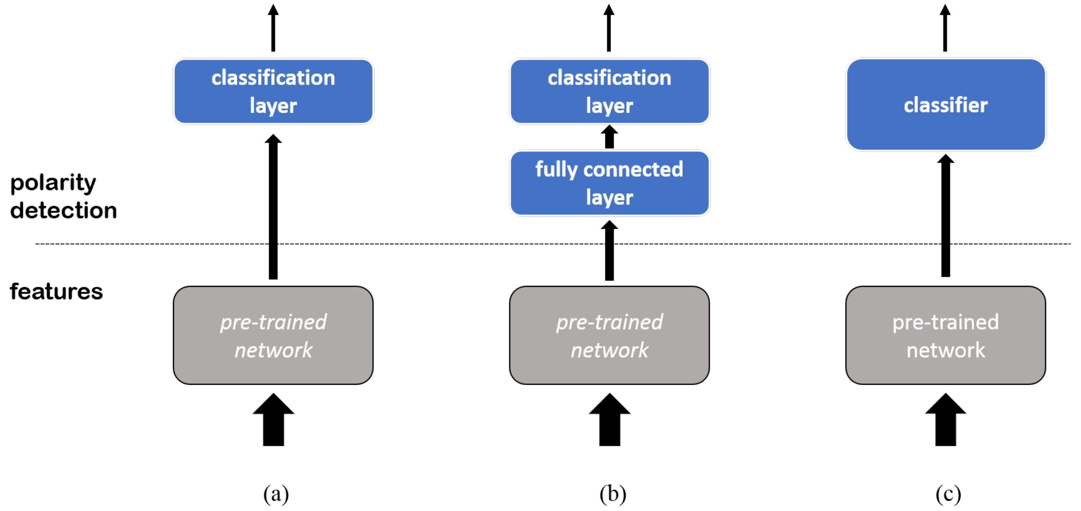
In all sessions, the layer replacement configuration was set up as follows. The optimization of the layer in the pre-trained CNN followed stochastic gradient descent with momentum, with momentum = $0.9$ and learning rate = ${10}^{-4}$. In the upper classification layer, the learning rate was ${10}^{-3}$ and the regularization parameter was $0.5$. The validation patience for early stopping was two. Training involved a maximum of 10 epochs.

The same setup was adopted for the layer addition configuration. In this case, the learning rate was ${10}^{-3}$, and the regularization parameter was 0.5 for both the fully-connected and the classification layer. Cross-validation drove the setting of the hyper-parameter, $N_h$, which could take on a discrete set of values: $N_h\in \{10,50,100,200\}$.

The classifier configuration did not require fine-tuning. The SVM with Gaussian kernel was trained with a standard algorithm. The two hyper-parameters, regularization term C and kernel standard deviation $\sigma$, were set via model selection.

6.3. Experimental Session #1

According to the proposed experimental design, eight different pre-trained architectures were used to generate as many implementations of each configuration. The experimental session aimed at comparing the generalization performances of such implementations.

For each configuration, the performances of the eight predictors were evaluated according to a five-fold strategy. Hence, for each dataset, the classification accuracy of a predictor was measured in five different experiments, corresponding to as many different splittings of the dataset into training/test pairs. Five separate runs of each single experiment were completed; each run involved a different composition of the mini-batch. As a result, for each predictor and each benchmark, 25 measurements of the classification accuracy on the test set were eventually available.

Table 5. Experimental results: Session #1, layer replacement.

Architecture	Tw	Mv_a	Mv_b	ANP40
AlexNet	82.5 (0.6)	66.2 (0.5)	65.4 (0.7)	76.3 (0.3)
Vgg_16	86.6 (0.4)	68.9 (1.0)	70.7 (1.0)	79.0 (0.3)
Vgg_19	86.4 (0.5)	69.2 (0.7)	$71.0$ (0.8)	78.7 (0.3)
GoogLeNet	84.2 (0.5)	66.0 (0.6)	68.2 (0.5)	79.2 (0.3)
Inc_v3	86.5 (0.7)	68.1 (0.7)	70.5 (0.9)	$79.9$ (0.2)
Res_50	85.8 (0.6)	68.9 (0.9)	68.8 (1.5)	79.2 (0.2)
Res_101	88.2 (0.4)	70.8 (0.6)	69.2 (0.8)	79.7 (0.2)
DenseNet	$89.4$ (0.5)	$71.3$ (0.8)	70.6 (0.6)	79.3 (0.3)

reports on the performances measured by applying the layer replacement configuration to Tw, Mv_a, Mv_b, and ANP40. The first column marks the pre-trained architecture used for implementing the predictor; the second column gives, for the Tw dataset, the average accuracy obtained by the predictor over the 25 experiments, together with its standard uncertainty (between brackets); the third, fourth, and fifth columns report the same quantities for the experiments on the Mv_a, Mv_b, and ANP40 datasets, respectively. Best results are marked in bold. The experimental outcomes proved that DenseNet slightly outperformed the other architectures on Tw and Mv_a. Vgg_19 scored the best average accuracy on Mv_b; the gap between such a predictor and Vgg_16, Inc_v3, and DenseNet though, was very small, especially if one considered the corresponding standard uncertainties. Furthermore, Res_101 always proved competitive with the best solution. At the same time, one can conclude that Inc_v3 and Res_101 proved the best predictors on ANP40. It is worth noting that seven predictors out of eight achieved an average accuracy in the percentage range [79.7, 78.7]; only the predictor based on AlexNet was slightly less effective on ANP40.

The results reported in Table 5 are consistent with those presented in the literature. Layer replacement was adopted in several frameworks for image polarity detection; most of the related works used the Tw dataset as a benchmark; hence, a direct comparison was feasible. In [44], an accuracy of $82\%$ was achieved with AlexNet, while in [13], Inc_v3 and Vgg_19 attained percentage accuracy scores of $86\%$ and $84\%$, respectively. These results indirectly confirm the reliability of the experimental setup adopted in this research.

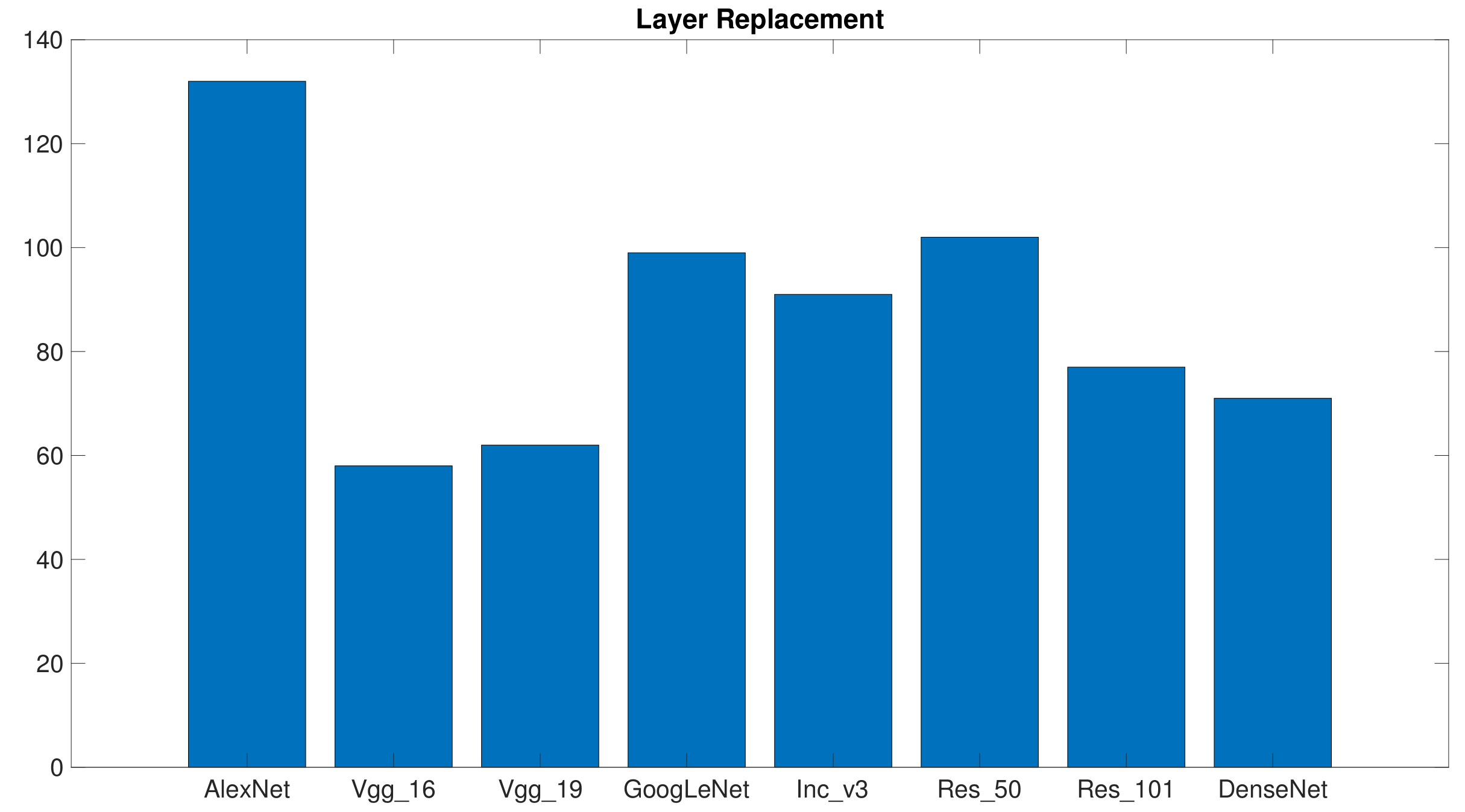
The experiments involving the layer replacement configurations could point out which architecture proved most consistent on the various dataset and the different training/set pairs. Thus, for each benchmark and for each training/set pair, the eight architectures were ranked according to the classification accuracy scored by the associated predictors. In this case, the accuracy score associated with a predictor was the best accuracy over the five runs completed for a given training/set pair. In each rank, one point was assigned to the best predictor, two points to the second best predictor, and so on, until the worst predictor, which took eight points. Figure 6 presents, for each architecture, the total points scored over the 20 ranks (5 training/test pairs × 4 benchmarks). In principle, a predictor could not mark less than 20 points, which would mean scoring first position (i.e., best predictor) for every rank. The graph shows that the predictors based on Vgg_16 and Vgg_19 resulted in being the most consistent. This outcome indeed reflected the results reported in Table 5, which showed that Vgg_16 and Vgg_19 always performed effectively on the different benchmarks. One should consider, however, that a classifier obtaining a good average accuracy might get a high score if the distribution of its accuracy is non-unimodal or its variance is high.

Table 6. Experimental results: Session #1, layer addition.

Architecture	Tw	Mv_a	Mv_b	ANP40
AlexNet	84.9 (0.4)	68.2 (0.4)	69.9 (0.7)	78.6 (0.2)
Vgg_16	88.0 (0.3)	70.9 (0.6)	72.3 (0.8)	80.0 (0.3)
Vgg_19	87.6 (0.4)	71.0 (0.7)	73.4 (0.6)	80.3 (0.2)
GoogLeNet	86.3 (0.3)	70.0 (0.4)	71.3 (0.5)	80.0 (0.3)
Inc_v3	85.3 (0.4)	66.4 (0.4)	68.5 (0.7)	80.3 (0.2)
Res_50	87.0 (0.3)	69.4 (0.6)	72.1 (0.8)	80.1 (0.2)
Res_101	89.1 (0.3)	72.1 (0.7)	$73.9$ (0.6)	80.2 (0.2)
DenseNet	$89.3$ (0.6)	70.9 (0.4)	71.2 (0.6)	$80.6$ (0.2)

reports on the performance obtained when applying the layer addition configuration on Tw, Mv_a, Mv_b, and ANP40. The Table follows the same format of Table 5. In each experiment, the training set was split into an actual training set and a validation set to support the model-selection procedure and set the hyperparameter $N_h$ in the eventual predictor. Experimental outcomes pointed out that Res_101 yielded the best average accuracy on Mv_a and Mv_b, whereas DenseNet achieved the best performance for Tw and ANP40. Overall, the gap with respect to the runner-up was always small, especially in the case of the experiments on Mv_b. On ANP40, seven predictors out of eight again achieved almost the same average accuracy. This confirmed that the availability of a large dataset somewhat counterbalanced the possible differences between the various comparisons. Noticeably, the predictors attained better average accuracy with the layer addition configuration than with the layer replacement setup. That improvement came at the cost of a more complex training procedure, as the layer addition configuration also required completing a model selection for setting $N_h$.

The layer replacement configuration did not allow a direct comparison with the frameworks published in the literature. The related frameworks typically adopted ad-hoc solutions for the design of the classification layer, whereas the present analysis required a standard solution for fair comparisons. Nevertheless, the literature seems to confirm that the best performances were obtained when using either VggNets or ResNets as feature extractors. 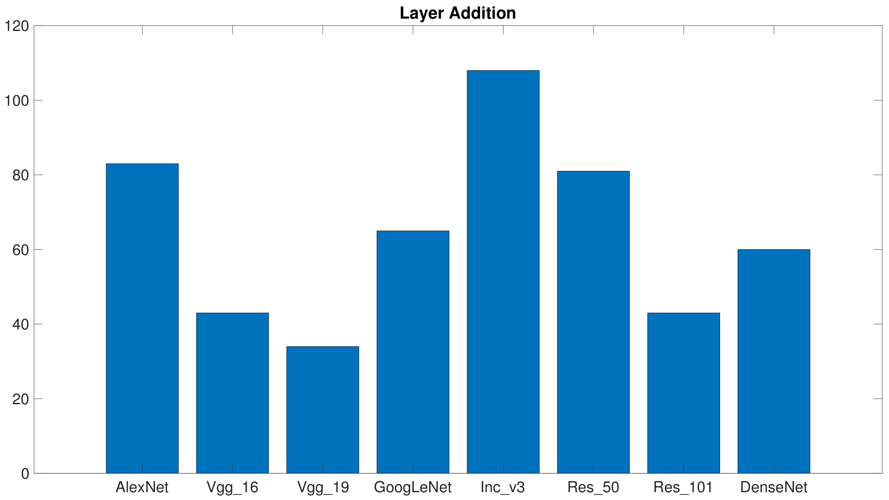Figure 7 provides the outcomes of the consistency assessment for the layer replacement configuration. The plot again gives, for each architecture, the total points marked over the 20 ranks (5 training/test pairs × 4 benchmarks). In this case, too, Vgg_19 proved to be the most consistent architecture, whereas Vgg_16 collected as much points as Res_101. These results are not in contrast to the results of Table 6; the practical hint is that classifiers based on Vgg_19 most likely lead to reliable predictors. Conversely, the chances reach a bad local minimum increase when Res_101 and DenseNet are involved in the training process.

Table 7. Experimental results: Session #1, classifier.

Architecture	Tw	Mv_a	Mv_b
AlexNet	80.7(3.7)	63.5(3.7)	70.2(1.0)
Vgg_16	$86.3\left(0.1\right)$	70.7(1.0)	70.4(2.3)
Vgg_19	85.3(1.3)	70.4(1.2)	73.3(1.6)
GoogLeNet	79.1(5.3)	67.7(1.3)	69.5(1.7)
Inc_v3	85.1(2.1)	72.1(0.9)	$75.2\left(1.7\right)$
Res_50	84.5(4.6)	72.4(2.3)	72.9(2.4)
Res_101	80.0(5.7)	70.5(1.6)	74.3(1.8)
DenseNet	85.0(4.8)	$72.5\left(1.0\right)$	70.2 (1.8)

reports on the performance obtained with the classification configuration on Tw, Mv_a, and Mv_b. The table follows the same format of Table 5. In this case, ANP40 was not included in the experiments, as (6) suggested that such a configuration should be avoided for computational reasons when large training sets are involved. The classification configuration required a model-selection procedure, as was the case for the layer addition configuration. Therefore, in each experiment, the training set was split into a training and a validation set to support the model-selection procedure to set up the hyperparameters C and $\sigma$ in the eventual predictors. Predictors based on the classification configuration could benefit from a convex optimization problem in the training phase; hence, the classification accuracy obtained with a given training/test pair could be estimated without resorting to multiple runs of the experiment. The table gives the average classification accuracy values over the five training/test pairs, together with the corresponding standard uncertainty. Experimental outcomes point out a few peculiarities of the classifier configuration, without fine-tuning. First, the predictor based on Res_101 never scored the best average accuracy; as a matter of fact, each benchmark witnessed a different winner. Secondly, the standard uncertainty associated with the average accuracy always was quite large. For each benchmark and each architecture, the variance of the accuracy over the five experiments always turned out to be quite wide; the composition of the training set played a major role. In practice, this meant that by adopting the classification configuration, one increases the risk of incurring a weak predictor, independently of the specific CNN architecture.

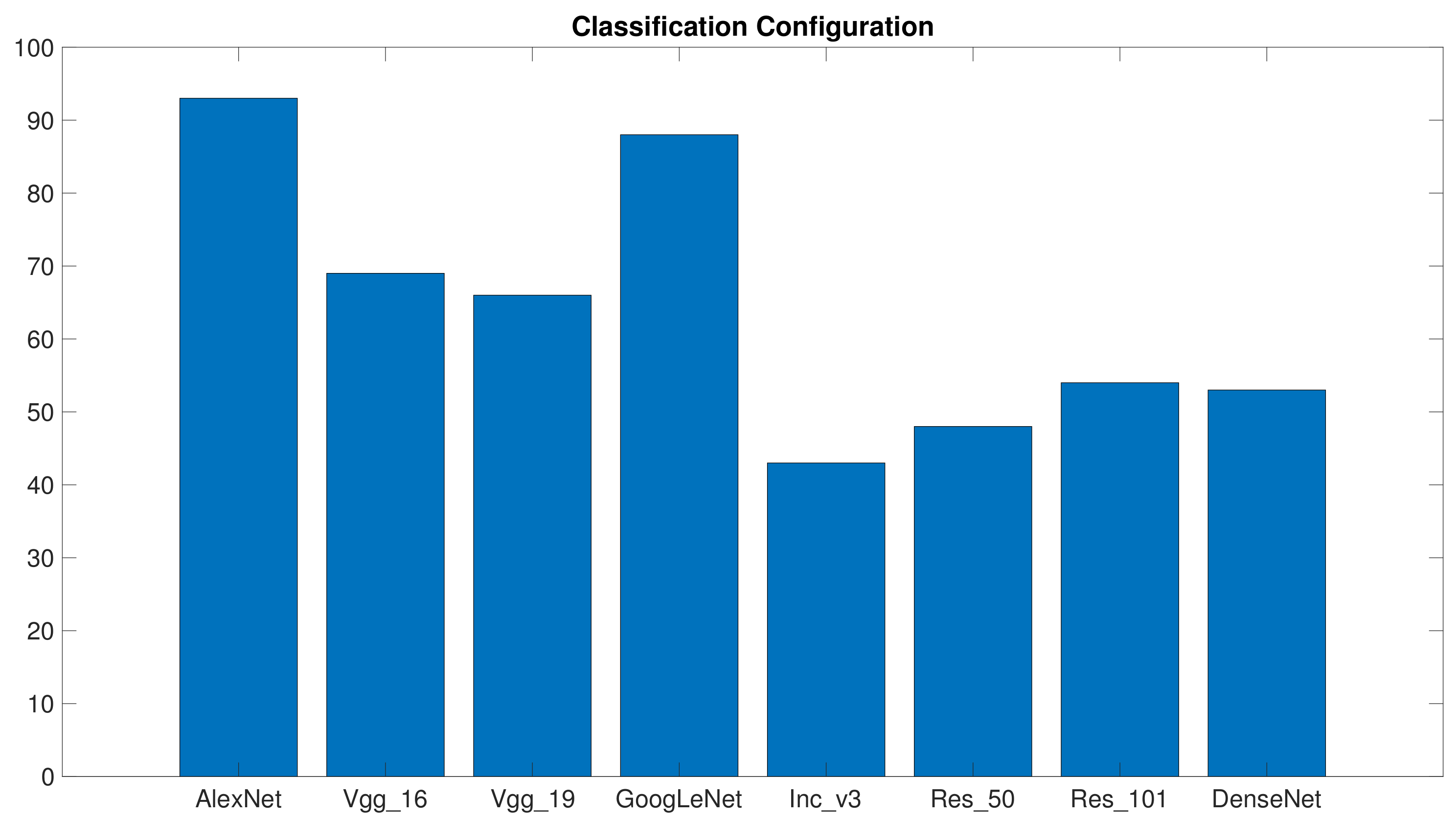
Figure 8 gives the consistency assessments for the classification configuration and follows the same format adopted in the previous graphs. The plot gives, for each architecture, the overall points scored in the 15 ranks (5 training/test pairs × 3 benchmarks). As expected, results differed significantly from those presented above: Res_50 and Inc_v3 proved to be the most consistent architectures, while Vgg_16 and Vgg_19 did not perform satisfactorily.

Interestingly, the Inc_v3 architecture did not attain good results when involved in the configurations requiring fine-tuning. Table 7 and Figure 8, though, suggest that Inc_v3 anyway represents a good starting point for image polarity detection. Making fine-tuning effective would require a more fine-grained selection of the optimizer hyper-parameters, but this would be paid at the cost of higher computational loads. As a result, the Inc_v3 architecture may not be compliant with the premises of this analysis.

6.4. Experimental Session #2

The dataset PT poses major challenges to polarity predictors, since a naive classifier that always predicts “positive” would achieve a 78% accuracy on this dataset. On the other hand, the literature proved that it is very difficult to attain a predictor that can discriminate effectively both classes in this benchmark.

The experimental session showed that neither the layer replacement configuration, nor the classification one could yield acceptable result on PT; the classifiers always featured accuracy values lower than $50\%$ for at least one of the two classes. Hence, this analysis will only consider the outcomes of the experiments with the layer addition configuration. The performances of the related eight predictors were evaluated by adopting a five-fold strategy. Accordingly, the classification accuracy of a predictor was detected in five different experiments. In each experiment, the original (imbalanced) training set was processed to obtain a more balanced set. For this purpose, oversampling [109] was applied to the negative (minority) class.

For each predictor, five separate runs of each five-fold experiment were carried out; this routine was repeated over the four admissible values of $N_h$. This procedure led to a total of 100 estimates of the test classification accuracy for each predictor.

Table 8. Experimental results: Session #2, layer addition.

Architecture	Successful Trials	Accuracy
AlexNet	4	66.5
Vgg_16	10	72.4
Vgg_19	5	72.6
GoogLeNet	8	67.0
Inc_v3	50	62.5
Res_50	45	69.7
Res_101	20	72.9
DenseNet	30	68.1

reports on the related outcomes and gives, for each predictor (first column), two quantities: the number of successful trials, i.e., the trials that led to a classification accuracy greater than 50% on both classes; the average accuracy over the number of successful trials. The empirical results suggest two remarks: Inc_v3 and Res_50 only achieved an acceptable share of successful trials. Secondly, Vgg_16, Vgg_19, and Res_101 outperformed the other comparisons in terms of average accuracy, in those few cases where successful trials were attained. In summary, the latter architectures were confirmed to be effective at polarity detection, but at the same time proved to be more prone to the problem of local minima.

The number of unsuccessful trials was in general quite high because the proposed dataset was very small and noisy. The purpose of this experiment was to evaluate the ability of the different configurations to learn complex rules with small training sets. Unsurprisingly, layer addition was the only configuration that obtained reasonable performance, possibly because it could train two layers from scratch. Layer replacement possibly failed because training just one layer from scratch would not render complex relationships adequately. The classification configurations relied on SVM, which embedded an inference function and the notion of the similarity between patterns. This might be a disadvantage when the number of training patterns is very small. In the case of layer addition, one should also take into account that the learning process strongly depends on the initial setup. In summary, Table 8 shows that the probability of reaching a good local minimum over 100 trails significantly varies with the CNN.

6.5. Computational Complexity: An Insight on the Role of CNNs

The experimental campaign showed that, overall, Vgg_16, Vgg_19, Res_101, and DenseNet proved to be the most reliable architectures in terms of generalization abilities. Computational aspects may be a discriminant factor, as the specific CNN determines the values assumed by $O_{ff}$ and $O_{bw}$ in (3) and (6) when targeting an implementation on GPUs.

The computational cost of the forward phase $O_{ff}$ is taken into consideration first. In terms of storage, i.e., number of parameters, the requirements by the pair of VggNet approaches were almost three- or four-times bigger than Res_101 and six- or eight-times bigger than DenseNet. Furthermore, the forward phase of VggNets involved two- or three-times the number of floating point operations as compared with Res_101. Notably, DenseNet used only 4 Gflops operations in the forward phase and would therefore appear as the best choice. On the other hand, in VggNets, most of the parameters and operations were introduced in the topmost fully-connected layers. As a result, these layers may take advantage of parallel computing, which can boost the overall efficiency when a sufficient amount of memory and computing units is available [110,111]. By contrast, both Res_101 and DenseNet exhibited a larger number of layers that needed to be computed sequentially; hence, the impact of parallel computing in improving their execution time is expected to be low. In conclusion, predictors based on Vgg_16 and Vgg_19 may represent the best option when the forward phase is allocated on a GPU with a considerable amount of memory. On the other hand, DenseNet seems preferable when one has to cope with memory constraints. Res_101 represents an intermediate solution.

Evaluating the cost of the back propagation phase $O_{bw}$ calls for a more detailed analysis. The classifier configuration does not require this phase; at the same time, the experimental campaign proved that better results can be obtained when fine-tuning is applied. For a qualitative analysis, the expression $O_{bw}\simeq 2O_{ff}$ provided a valid approximation. The actual proportion, though, can substantially differ when considering that deep CNNs are complex models involving different types of blocks. Approximations of computational costs often disregard the contributions of components such as ReLU, pooling, and batch normalization (BN) layers [108]. However, such a simplification gets less reliable in the presence of more and more complex, non-convolutional, or fully-connected layers. This issue shows up in the analysis proposed in [108], which is summarizes in

Table 9. Computational time trade off between convolutional and fully-connected layer versus other layer topologies [108].

Architectures	Vgg_19	Res_50	DenseNet_121
CONV/FC	95.1%	61.9%	41.5%
non-CONV/non-FC	4.9%	38.1%	58.5%

. The table compares the three architectures involved in the present evaluation, VggNet, ResNet, and DenseNet. For each architecture, the first row gives the percentages of time spent in convolutions and fully-connected layers; the second row gives the computing time percentage of time spent in the remaining layers. Even if the experiments in [108] did not address exactly Res_101 and Dense_201, one can reasonably assume that the same trend applies to those networks, as well. In conclusion, the approximation $O_{bw}\simeq 2O_{ff}$ becomes less reliable as long as newer models are proposed. For instance, batch normalization units play a crucial role in the training phase of the ResNet and DenseNet architectures (as per Table 9), but these logical blocks are not included in the eventual predictors. This in turn means that $O_{ff}$ is definitely lighter than $O_{bw}$.

The memory consumption during the training phase is an additional significant factor. Storage is nonlinear with respect to the number of parameters and is strongly influenced by the number of connections within the network. It is well known that deeper and thinner networks are less efficient in terms of parallelism and memory consumption as compared with structures with less, but wider, layers. An intuitive explanation is that, during back propagation, the output of each layer needs to be stored; hence, the memory requirement grows as the number of layers grow. Most existing implementations of DenseNet require indeed an amount of memory that grows quadratically with the number of layers, even if DenseNet involves a small number of parameters as compared with the other comparisons. Nonetheless, ad-hoc implementations of DenseNet exist that make the growth linear [112].

Overall, the plain implementation of the VggNets might result in being simpler than the plain implementation of Res_101 and DenseNet. On the other hand, an optimized implementation of DenseNet and Res_101 could attain valuable improvement in terms of performances. Anyway, one should always take into account that layers must be executed in sequential order; hence, the depth of the network impacts latency.

7. Concluding Remarks and Discussion

This paper evaluated the role played by CNNs and transfer learning in image polarity detection. The experimental protocol considered three configurations of the predictors, which covered the most significant approaches proposed in the literature. The predictors were analyzed and compared in terms of both generalization performance and computational complexity. The former issue is critical because image-polarity detection applications usually involve limited datasets; at the same time, computational costs may represent a key factor when the implementation of the prediction system is targeted to an electronic device. The experimental outcomes of the protocol yielded useful insights on the network architectures, the predictor’s configurations, and the underlying fine-tuning strategies.

Layer addition proved most effective in terms of classification accuracy. That approach, however, also turned out to be the most computationally demanding, as the training process involved both the back propagation for weight adjustment and the model selection procedure to support the setup of $N_h$. Besides, the regularization parameter actually played the role of a hyperparameter. In this work, this quantity was always set to 0.5, mostly for exploiting the regularization properties of early stopping. On the other hand, by a proper model selection, one could boost the generalization performance, at the cost of an increased computational load.

The classifier configuration represents the most convenient option from the computational point of view. In contrast, this approach proved to be possibly too sensitive to the composition of the training set, which might make this approach impractical in real-word scenarios.

Conversely, the layer replacement configuration achieved a satisfactory balance between accuracy, convergence in the training process, and computational cost. It is worth noting that the training procedure of both the layer replacement and the layer addition solutions can be simplified by inhibiting fine-tuning in the lowest layers of the CNN, and only involving the upper layers of either architecture in the training process. The experimental protocol did not explore this setup because the networks differed significantly in the number of layers (from 8 to 101), so a fair comparison would be difficult.

The results of the experimental section were consistent with the trend presented in the literature: the frameworks that did not augment the original object detection architecture by fine-tuning were generally lower performing. The layer replacement option can be considered a simplified version of models that employ sophisticated configurations to process the features extracted by retrained CNNs for object detection.

The architectures Vgg_16, Vgg_19, Res_101, and DenseNet proved to be the most robust options in terms of generalization abilities; hence, the computational impact may become the discriminative criteria. The Vgg_16 and Vgg_19 architectures are “shallow and wide”, whereas Res_101 and DenseNet can be regarded as “deep and thin” structures. Thus, the VggNet architectures can most benefit from the advantages of parallel computing; conversely, Res_101 and DenseNet feature complex structures that require careful implementations.

Image polarity detection is a young research field; hence, many important issues still remain open. Deep learning is by all means contributing to making polarity detectors very reliable. A very interesting research direction is the development of models capable of locating the most important regions in an image, to exploit saliency to improve sentiment analysis [48,54,55,56,57,58]. Up to now, multi-task learning has received little attention, although several applications exist that require solving multiple visual tasks. Autonomous interactive robots, for instance, might need to combine object classification and image polarity detection. Finally, more attention should be dedicated in the future to the deployment of image polarity detection models that can be hosted on embedded systems. In this regard, it could be interesting to take advantage of multi-objective optimization to design cost-sensitive loss functions.

References

1. Soleymani, M.; Garcia, D.; Jou, B.; Schuller, B.; Chang, S.F.; Pantic, M. A survey of multimodal sentiment analysis. Image Vis. Comput. 2017, 65, 3–14. [Google Scholar] [CrossRef]
2. Poria, S.; Cambria, E.; Bajpai, R.; Hussain, A. A review of affective computing: From unimodal analysis to multimodal fusion. Inf. Fusion 2017, 37, 98–125. [Google Scholar] [CrossRef] [Green Version]
3. Hazarika, D.; Poria, S.; Zadeh, A.; Cambria, E.; Morency, L.P.; Zimmermann, R. Conversational memory network for emotion recognition in dyadic dialogue videos. In Proceedings of the 2018 Conference of the North American Chapter of the Association for Computational Linguistics: Human Language Technologies, New Orleans, LA, USA, 1–6 June 2018; Volume 1, pp. 2122–2132. [Google Scholar]
4. Cambria, E.; Hussain, A.; Havasi, C.; Eckl, C. Sentic Space: Visualizing Opinions and Sentiments in a Multi-Dimensional Vector Space. In Knowledge-Based and Intelligent Information and Engineering Systems; Setchi, R., Jordanov, I., Howlett, R., Jain, L., Eds.; Springer: Berlin, Germany, 2010; Volume 6279, pp. 385–393. [Google Scholar]
5. Cambria, E.; Olsher, D.; Kwok, K. Sentic Activation: A Two-Level Affective Common Sense Reasoning Framework. In Proceedings of the Twenty-Sixth AAAI Conference on Artificial Intelligence, Toronto, ON, USA, 22–26 July 2012; pp. 186–192. [Google Scholar]
6. Ducange, P.; Fazzolari, M.; Petrocchi, M.; Vecchio, M. An effective Decision Support System for social media listening based on cross-source sentiment analysis models. Eng. Appl. Artif. Intell. 2019, 78, 71–85. [Google Scholar] [CrossRef]
7. Cambria, E.; Hussain, A.; Durrani, T.; Havasi, C.; Eckl, C.; Munro, J. Sentic Computing for Patient Centered Application. In Proceedings of the IEEE 10th International Conference on Signal Processing, Beijing, China, 24–28 October 2010; pp. 1279–1282. [Google Scholar]
8. Cambria, E. An Introduction to Concept-Level Sentiment Analysis. In Advances in Soft Computing and Its Applications; Castro, F., Gelbukh, A., González, M., Eds.; Springer-Verlag: Berlin, Germany, 2013; Volume 8266, pp. 478–483. [Google Scholar]
9. Perikos, I.; Hatzilygeroudis, I. Recognizing emotions in text using ensemble of classifiers. Eng. Appl. Artif. Intell. 2016, 51, 191–201. [Google Scholar] [CrossRef]
10. Fang, Y.; Chen, X.; Song, Z.; Wang, T.; Cao, Y. Modelling Propagation of Public Opinions on Microblogging Big Data Using Sentiment Analysis and Compartmental Models. Int. J. Semant. Web Inf. Syst. 2017, 13, 11–27. [Google Scholar] [CrossRef]
11. Xu, C.; Cetintas, S.; Lee, K.C.; Li, L.J. Visual sentiment prediction with deep convolutional neural networks. arXiv 2014, arXiv:1411.5731. [Google Scholar]
12. You, Q.; Luo, J.; Jin, H.; Yang, J. Robust Image Sentiment Analysis Using Progressively Trained and Domain Transferred Deep Networks. In Proceedings of the Twenty-Ninth AAAI Conference on Artificial Intelligence, Austin, TX, USA, 25–30 January 2015; pp. 381–388. [Google Scholar]
13. Islam, J.; Zhang, Y. Visual sentiment analysis for social images using transfer learning approach. In Proceedings of the 2016 IEEE International Conferences on Big Data and Cloud Computing (BDCloud), Social Computing and Networking (SocialCom), Sustainable Computing and Communications (SustainCom)(BDCloud-SocialCom-SustainCom), Atlanta, GA, USA, 8–10 October 2016; pp. 124–130. [Google Scholar]
14. Campos, V.; Jou, B.; Giro-i Nieto, X. From pixels to sentiment: Fine-tuning cnns for visual sentiment prediction. Image Vis. Comput. 2017, 65, 15–22. [Google Scholar] [CrossRef]
15. Alom, M.Z.; Taha, T.M.; Yakopcic, C.; Westberg, S.; Sidike, P.; Nasrin, M.S.; Hasan, M.; Van Essen, B.C.; Awwal, A.A.; Asari, V.K. A State-of-the-Art Survey on Deep Learning Theory and Architectures. Electronics 2019, 8, 292. [Google Scholar] [CrossRef]
16. Luo, J.; Borth, D.; You, Q. Social Multimedia Sentiment Analysis. In Proceedings of the 2017 ACM on Multimedia Conference, Mountain View, CA, USA, 23–27 October 2017; pp. 1953–1954. [Google Scholar]
17. Zhao, S.; Ding, G.; Huang, Q.; Chua, T.S.; Schuller, B.W.; Keutzer, K. Affective Image Content Analysis: A Comprehensive Survey. In Proceedings of the Twenty-Seventh International Joint Conference on Artificial Intelligence (IJCAI-18), Stockholm, Sweden, 13–19 July 2018; pp. 5534–5541. [Google Scholar]
18. Hatcher, W.G.; Yu, W. A survey of deep learning: Platforms, applications and emerging research trends. IEEE Access 2018, 6, 24411–24432. [Google Scholar] [CrossRef]
19. Esteva, A.; Robicquet, A.; Ramsundar, B.; Kuleshov, V.; DePristo, M.; Chou, K.; Cui, C.; Corrado, G.; Thrun, S.; Dean, J. A guide to deep learning in healthcare. Nat. Med. 2019, 25, 24. [Google Scholar] [CrossRef]
20. Fawaz, H.I.; Forestier, G.; Weber, J.; Idoumghar, L.; Muller, P.A. Deep learning for time series classification: A review. Data Min. Knowl. Discov. 2019, 33, 917–963. [Google Scholar] [CrossRef]
21. Zhao, Z.Q.; Zheng, P.; Xu, S.T.; Wu, X. Object detection with deep learning: A review. IEEE Trans. Neural Netw. Learn. Syst. 2019, 1–21. [Google Scholar] [CrossRef] [PubMed]
22. Borth, D.; Ji, R.; Chen, T.; Breuel, T.; Chang, S.F. Large-scale visual sentiment ontology and detectors using adjective noun pairs. In Proceedings of the 21st ACM International Conference on Multimedia, Barcelona, Spain, 21–25 October 2013; pp. 223–232. [Google Scholar]
23. Yosinski, J.; Clune, J.; Bengio, Y.; Lipson, H. How transferable are features in deep neural networks. In Advances in Neural Information Processing Systems; Curran Associates, Inc.: New York, NY, USA, 2014; pp. 3320–3328. [Google Scholar]
24. Pan, S.J.; Yang, Q. A survey on transfer learning. IEEE Trans. Knowl. Data Eng. 2010, 22, 1345–1359. [Google Scholar] [CrossRef]
25. Weiss, K.; Khoshgoftaar, T.M.; Wang, D. A survey of transfer learning. J. Big Data 2016, 3, 9. [Google Scholar] [CrossRef]
26. Krizhevsky, A.; Sutskever, I.; Hinton, G.E. Imagenet classification with deep convolutional neural networks. In Advances in Neural Information Processing Systems; Curran Associates, Inc.: New York, NY, USA, 2012; pp. 1097–1105. [Google Scholar]
27. Simonyan, K.; Zisserman, A. Very deep convolutional networks for large-scale image recognition. arXiv 2014, arXiv:1409.1556. [Google Scholar]
28. Szegedy, C.; Liu, W.; Jia, Y.; Sermanet, P.; Reed, S.; Anguelov, D.; Erhan, D.; Vanhoucke, V.; Rabinovich, A. Going deeper with convolutions. In Proceedings of the IEEE Conference on Computer Vision and Pattern Recognition, Boston, MA, USA, 7–12 June 2015; pp. 1–9. [Google Scholar]
29. Szegedy, C.; Vanhoucke, V.; Ioffe, S.; Shlens, J.; Wojna, Z. Rethinking the inception architecture for computer vision. In Proceedings of the IEEE Conference on Computer Vision and Pattern Recognition, Las Vegas, NV, USA, 27–30 June 2016; pp. 2818–2826. [Google Scholar]
30. Szegedy, C.; Ioffe, S.; Vanhoucke, V.; Alemi, A.A. Inception-v4, inception-resnet and the impact of residual connections on learning. In Proceedings of the Thirty-First AAAI Conference on Artificial Intelligence, San Francisco, CA, USA, 4–9 February 2017; Volume 4, p. 12. [Google Scholar]
31. He, K.; Zhang, X.; Ren, S.; Sun, J. Deep residual learning for image recognition. In Proceedings of the IEEE Conference on Computer Vision and Pattern Recognition, Las Vegas, NV, USA, 27–30 June 2016; pp. 770–778. [Google Scholar]
32. Huang, G.; Liu, Z.; Van Der Maaten, L.; Weinberger, K.Q. Densely Connected Convolutional Networks. In Proceedings of the IEEE Conference on Computer Vision and Pattern Recognition, Honolulu, HI, USA, 21–26 July 2017; Volume 1, pp. 4700–4708. [Google Scholar]
33. Russakovsky, O.; Deng, J.; Su, H.; Krause, J.; Satheesh, S.; Ma, S.; Huang, Z.; Karpathy, A.; Khosla, A.; Bernstein, M.; et al. Imagenet large scale visual recognition challenge. Int. J. Comput. Vis. 2015, 115, 211–252. [Google Scholar] [CrossRef]
34. Canziani, A.; Paszke, A.; Culurciello, E. An analysis of deep neural network models for practical applications. arXiv 2016, arXiv:1605.07678. [Google Scholar]
35. Wei-ning, W.; Ying-lin, Y.; Sheng-ming, J. Image retrieval by emotional semantics: A study of emotional space and feature extraction. In Proceedings of the 2006 IEEE International Conference on Systems, Man and Cybernetics, Taipei, Taiwan, 8–11 October 2006; Volume 4, pp. 3534–3539. [Google Scholar]
36. Siersdorfer, S.; Minack, E.; Deng, F.; Hare, J. Analyzing and predicting sentiment of images on the social web. In Proceedings of the 18th ACM International Conference on Multimedia, Firenze, Italy, 25–29 October 2010; ACM: New York, NY, USA, 2010; pp. 715–718. [Google Scholar] [Green Version]
37. Machajdik, J.; Hanbury, A. Affective image classification using features inspired by psychology and art theory. In Proceedings of the 18th ACM International Conference on Multimedia, Firenze, Italy, 25–29 October 2010; ACM: New York, NY, USA, 2010; pp. 83–92. [Google Scholar]
38. Yanulevskaya, V.; van Gemert, J.C.; Roth, K.; Herbold, A.K.; Sebe, N.; Geusebroek, J.M. Emotional valence categorization using holistic image features. In Proceedings of the 2008 15th IEEE International Conference on Image Processing, San Diego, CA, USA, 12–15 October 2008; pp. 101–104. [Google Scholar]
39. Peng, K.C.; Chen, T.; Sadovnik, A.; Gallagher, A.C. A mixed bag of emotions: Model, predict, and transfer emotion distributions. In Proceedings of the IEEE Conference on Computer Vision and Pattern Recognition, Boston, MA, USA, 7–12 June 2015; pp. 860–868. [Google Scholar]
40. Yuan, J.; Mcdonough, S.; You, Q.; Luo, J. Sentribute: Image sentiment analysis from a mid-level perspective. In Proceedings of the Second International Workshop on Issues of Sentiment Discovery and Opinion Mining, Chicago, IL, USA, 11–14 August 2013; p. 10. [Google Scholar]
41. Nicolaou, M.A.; Gunes, H.; Pantic, M. A multi-layer hybrid framework for dimensional emotion classification. In Proceedings of the 19th ACM International Conference on Multimedia, Scottsdale, AZ, USA, 28 November–1 December 2011; pp. 933–936. [Google Scholar]
42. Solli, M.; Lenz, R. Color based bags-of-emotions. In International Conference on Computer Analysis of Images and Patterns; Springer: Berlin, Germany, 2009; pp. 573–580. [Google Scholar]
43. Chen, T.; Yu, F.X.; Chen, J.; Cui, Y.; Chen, Y.Y.; Chang, S.F. Object-based visual sentiment concept analysis and application. In Proceedings of the 22nd ACM International Conference on Multimedia, Orlando, FL, USA, 3–7 November 2014; pp. 367–376. [Google Scholar]
44. Campos, V.; Salvador, A.; Giro-i Nieto, X.; Jou, B. Diving deep into sentiment: Understanding fine-tuned cnns for visual sentiment prediction. In Proceedings of the 1st International Workshop on Affect & Sentiment in Multimedia, Brisbane, Australia, 26–30 October 2015; pp. 57–62. [Google Scholar]
45. Chen, T.; Borth, D.; Darrell, T.; Chang, S.F. Deepsentibank: Visual sentiment concept classification with deep convolutional neural networks. arXiv 2014, arXiv:1410.8586. [Google Scholar]
46. Talavera, E.; Radeva, P.; Petkov, N. Towards egocentric sentiment analysis. In International Conference on Computer Aided Systems Theory; Springer: Las Palmas de Gran Canaria, Spain, 2017; pp. 297–305. [Google Scholar]
47. Jou, B.; Chen, T.; Pappas, N.; Redi, M.; Topkara, M.; Chang, S.F. Visual affect around the world: A large-scale multilingual visual sentiment ontology. In Proceedings of the 23rd ACM International Conference on Multimedia, Brisbane, Australia, 26–30 October 2015; pp. 159–168. [Google Scholar]
48. Fan, S.; Jiang, M.; Shen, Z.; Koenig, B.L.; Kankanhalli, M.S.; Zhao, Q. The Role of Visual Attention in Sentiment Prediction. In Proceedings of the 2017 ACM on Multimedia Conference, Mountain View, CA, USA, 23–27 October 2017; pp. 217–225. [Google Scholar]
49. De Oliveira, W.B.; Dorini, L.B.; Minetto, R.; Silva, T.H. OutdoorSent: Can Semantic Features Help Deep Learning in Sentiment Analysis of Outdoor Images? arXiv 2019, arXiv:1906.02331. [Google Scholar]
50. Fernandez, D.; Woodward, A.; Campos, V.; Giró-i Nieto, X.; Jou, B.; Chang, S.F. More Cat than Cute?: Interpretable Prediction of Adjective-Noun Pairs. In Proceedings of the Workshop on Multimodal Understanding of Social, Affective and Subjective Attributes, Mountain View, CA, USA, 23–27 October 2017; pp. 61–69. [Google Scholar]
51. Narihira, T.; Borth, D.; Yu, S.X.; Ni, K.; Darrell, T. Mapping Images to Sentiment Adjective Noun Pairs with Factorized Neural Nets. arXiv 2015, arXiv:1511.06838. [Google Scholar]
52. Wang, J.; Fu, J.; Xu, Y.; Mei, T. Beyond Object Recognition: Visual Sentiment Analysis with Deep Coupled Adjective and Noun Neural Networks. In Proceedings of the Twenty-Fifth International Joint Conference on Artificial Intelligence, New York, NY, USA, 9–15 July 2016; pp. 3484–3490. [Google Scholar]
53. Jou, B.; Chang, S.F. Deep cross residual learning for multitask visual recognition. In Proceedings of the 2016 ACM on Multimedia Conference, Amsterdam, The Netherlands, 15–19 October 2016; pp. 998–1007. [Google Scholar]
54. Zheng, H.; Chen, T.; You, Q.; Luo, J. When saliency meets sentiment: Understanding how image content invokes emotion and sentiment. In Proceedings of the 2017 IEEE International Conference on Image Processing (ICIP), Beijing, China, 17–20 September 2017; pp. 630–634. [Google Scholar]
55. Wu, L.; Qi, M.; Jian, M.; Zhang, H. Visual Sentiment Analysis by Combining Global and Local Information. Neural Process. Lett. 2019, 1–13. [Google Scholar] [CrossRef]
56. Mnih, V.; Heess, N.; Graves, A.; Kavukcuoglu, K. Recurrent models of visual attention. In Advances in Neural Information Processing Systems; Curran Associates, Inc.: New York, NY, USA, 2014; pp. 2204–2212. [Google Scholar]
57. Sun, M.; Yang, J.; Wang, K.; Shen, H. Discovering affective regions in deep convolutional neural networks for visual sentiment prediction. In Proceedings of the 2016 IEEE International Conference on Multimedia and Expo (ICME), Seattle, WA, USA, 11–15 July 2016; pp. 1–6. [Google Scholar]
58. You, Q.; Jin, H.; Luo, J. Visual Sentiment Analysis by Attending on Local Image Regions. In Proceedings of the Thirty-First AAAI Conference on Artificial Intelligence, San Francisco, CA, USA, 4–9 February 2017; pp. 231–237. [Google Scholar]
59. Yang, J.; She, D.; Sun, M.; Cheng, M.M.; Rosin, P.; Wang, L. Visual sentiment prediction based on automatic discovery of affective regions. IEEE Trans. Multimedia 2018, 20, 2513–2525. [Google Scholar] [CrossRef]
60. Yang, J.; She, D.; Lai, Y.K.; Rosin, P.L.; Yang, M.H. Weakly Supervised Coupled Networks for Visual Sentiment Analysis. In Proceedings of the IEEE Conference on Computer Vision and Pattern Recognition, Salt Lake City, UT, USA, 18–22 June 2018; pp. 7584–7592. [Google Scholar]
61. Rao, T.; Li, X.; Zhang, H.; Xu, M. Multi-level region-based Convolutional Neural Network for image emotion classification. Neurocomputing 2019, 333, 429–439. [Google Scholar] [CrossRef]
62. Song, K.; Yao, T.; Ling, Q.; Mei, T. Boosting Image Sentiment Analysis with Visual Attention. Neurocomputing 2018, 312, 218–228. [Google Scholar] [CrossRef]
63. Liu, X.; Li, N.; Xia, Y. Affective image classification by jointly using interpretable art features and semantic annotations. J. Vis. Commun. Image Represent. 2019, 58, 576–588. [Google Scholar] [CrossRef]
64. Liu, A.; Shi, Y.; Jing, P.; Liu, J.; Su, Y. Structured low-rank inverse-covariance estimation for visual sentiment distribution prediction. Signal Process. 2018, 152, 206–216. [Google Scholar] [CrossRef]
65. Balouchian, P.; Foroosh, H. Context-Sensitive Single-Modality Image Emotion Analysis: A Unified Architecture from Dataset Construction to CNN Classification. In Proceedings of the 2018 25th IEEE International Conference on Image Processing (ICIP), Athens, Greece, 7–10 October 2018; pp. 1932–1936. [Google Scholar]
66. Karpathy, A.; Fei-Fei, L. Deep visual-semantic alignments for generating image descriptions. In Proceedings of the IEEE Conference on Computer Vision and Pattern Recognition, Boston, MA, USA, 7–12 June 2015; pp. 3128–3137. [Google Scholar]
67. Chung, J.; Gulcehre, C.; Cho, K.; Bengio, Y. Empirical evaluation of gated recurrent neural networks on sequence modeling. arXiv 2014, arXiv:1412.3555. [Google Scholar]
68. Mathews, A.P.; Xie, L.; He, X. SentiCap: Generating Image Descriptions with Sentiments. In Proceedings of the Thirtieth AAAI Conference on Artificial Intelligence, Phoenix, AZ, USA, 12–17 February 2016; pp. 3574–3580. [Google Scholar]
69. Shin, A.; Ushiku, Y.; Harada, T. Image Captioning with Sentiment Terms via Weakly-Supervised Sentiment Dataset. In Proceedings of the British Machine Vision Conference 2016, York, UK, 19–22 September 2016. [Google Scholar]
70. Yang, J.; Sun, Y.; Liang, J.; Ren, B.; Lai, S.H. Image captioning by incorporating affective concepts learned from both visual and textual components. Neurocomputing 2019, 328, 56–68. [Google Scholar] [CrossRef]
71. You, Q.; Jin, H.; Luo, J. Image Captioning at Will: A Versatile Scheme for Effectively Injecting Sentiments into Image Descriptions. arXiv 2018, arXiv:1801.10121. [Google Scholar]
72. Karayil, T.; Blandfort, P.; Borth, D.; Dengel, A. Generating Affective Captions using Concept And Syntax Transition Networks. In Proceedings of the 2016 ACM on Multimedia Conference, Amsterdam, The Netherlands, 15–19 October 2016; pp. 1111–1115. [Google Scholar]
73. Sun, Y.; Ren, B. Automatic Image Description Generation with Emotional Classifiers. In CCF Chinese Conference on Computer Vision; Springer Nature Switzerland AG: Tianjin, China, 2017; pp. 748–763. [Google Scholar]
74. Niu, T.; Zhu, S.; Pang, L.; El Saddik, A. Sentiment analysis on multi-view social data. In International Conference on Multimedia Modeling; Springer Nature Switzerland AG: Miami, FL, USA, 2016; pp. 15–27. [Google Scholar]
75. Guillaumin, M.; Verbeek, J.; Schmid, C. Multimodal semi-supervised learning for image classification. In Proceedings of the 2010 IEEE Conference on Computer Vision and Pattern Recognition (CVPR), San Francisco, CA, USA, 13–18 June 2010; pp. 902–909. [Google Scholar]
76. Katsurai, M.; Satoh, S. Image sentiment analysis using latent correlations among visual, textual, and sentiment views. In Proceedings of the 2016 IEEE International Conference on Acoustics, Speech and Signal Processing (ICASSP), Shanghai, China, 20–25 March 2016; pp. 2837–2841. [Google Scholar]
77. Gong, Y.; Ke, Q.; Isard, M.; Lazebnik, S. A multi-view embedding space for modeling internet images, tags, and their semantics. Int. J. Comput. Vis. 2014, 106, 210–233. [Google Scholar] [CrossRef]
78. Cai, G.; Xia, B. Convolutional neural networks for multimedia sentiment analysis. In Natural Language Processing and Chinese Computing; Springer Nature Switzerland AG: Nanchang, China, 2015; pp. 159–167. [Google Scholar]
79. Malatesta, L.; Asteriadis, S.; Caridakis, G.; Vasalou, A.; Karpouzis, K. Associating gesture expressivity with affective representations. Eng. Appl. Artif. Intell. 2016, 51, 124–135. [Google Scholar] [CrossRef]
80. You, Q. Sentiment and emotion analysis for social multimedia: Methodologies and applications. In Proceedings of the 2016 ACM on Multimedia Conference, Amsterdam, The Netherlands, 15–19 October 2016; pp. 1445–1449. [Google Scholar]
81. You, Q.; Luo, J.; Jin, H.; Yang, J. Joint visual-textual sentiment analysis with deep neural networks. In Proceedings of the 23rd ACM International Conference on Multimedia, Brisbane, Australia, 26–30 October 2015; pp. 1071–1074. [Google Scholar]
82. Chen, X.; Wang, Y.; Liu, Q. Visual and Textual Sentiment Analysis Using Deep Fusion Convolutional Neural Networks. arXiv 2017, arXiv:1711.07798. [Google Scholar]
83. Chen, F.; Ji, R.; Su, J.; Cao, D.; Gao, Y. Predicting Microblog Sentiments via Weakly Supervised Multimodal Deep Learning. IEEE Trans. Multimed. 2018, 20, 997–1007. [Google Scholar] [CrossRef]
84. Huang, F.; Zhang, X.; Zhao, Z.; Xu, J.; Li, Z. Image–text sentiment analysis via deep multimodal attentive fusion. Knowl. Based Syst. 2019, 167, 26–37. [Google Scholar] [CrossRef]
85. Xu, J.; Huang, F.; Zhang, X.; Wang, S.; Li, C.; Li, Z.; He, Y. Sentiment analysis of social images via hierarchical deep fusion of content and links. Appl. Soft Comput. 2019, 80, 387–399. [Google Scholar] [CrossRef]
86. Zhao, S.; Ding, G.; Gao, Y.; Han, J. Learning Visual Emotion Distributions via Multi-Modal Features Fusion. In Proceedings of the 2017 ACM on Multimedia Conference, Mountain View, CA, USA, 23–27 October 2017; pp. 369–377. [Google Scholar]
87. Yang, J.; Sun, M.; Sun, X. Learning Visual Sentiment Distributions via Augmented Conditional Probability Neural Network. In Proceedings of the Thirty-First AAAI Conference on Artificial Intelligence, San Francisco, CA, USA, 4–9 February 2017; pp. 224–230. [Google Scholar]
88. Yang, J.; She, D.; Sun, M. Joint image emotion classification and distribution learning via deep convolutional neural network. In Proceedings of the 26th International Joint Conference on Artificial Intelligence, Melbourne, Australia, 19–25 August 2017; pp. 3266–3272. [Google Scholar]
89. He, X.; Zhang, W. Emotion recognition by assisted learning with convolutional neural networks. Neurocomputing 2018, 291, 187–194. [Google Scholar] [CrossRef]
90. Zhao, S.; Ding, G.; Gao, Y.; Zhao, X.; Tang, Y.; Han, J.; Yao, H.; Huang, Q. Discrete Probability Distribution Prediction of Image Emotions With Shared Sparse Learning. IEEE Trans. Affect. Comput. 2018, 1. [Google Scholar] [CrossRef]
91. Zhao, S.; Yao, H.; Jiang, X.; Sun, X. Predicting discrete probability distribution of image emotions. In Proceedings of the 2015 IEEE International Conference on Image Processing (ICIP), Quebec City, QC, Canada, 27–30 September 2015; pp. 2459–2463. [Google Scholar]
92. Zhao, S.; Yao, H.; Gao, Y.; Ding, G.; Chua, T.S. Predicting personalized image emotion perceptions in social networks. IEEE Trans. Affect. Comput. 2016, 9, 526–540. [Google Scholar] [CrossRef]
93. Zhao, S.; Zhao, X.; Ding, G.; Keutzer, K. EmotionGAN: Unsupervised Domain Adaptation for Learning Discrete Probability Distributions of Image Emotions. In Proceedings of the 2018 ACM Conference on Multimedia, Seoul, Korea, 22–26 October 2018; pp. 1319–1327. [Google Scholar]
94. Sariyanidi, E.; Gunes, H.; Cavallaro, A. Automatic analysis of facial affect: A survey of registration, representation, and recognition. IEEE Trans. Pattern Anal. Mach. Intell. 2015, 37, 1113–1133. [Google Scholar] [CrossRef]
95. Kaltwang, S.; Todorovic, S.; Pantic, M. Doubly sparse relevance vector machine for continuous facial behavior estimation. IEEE Trans. Pattern Anal. Mach. Intell. 2016, 38, 1748–1761. [Google Scholar] [CrossRef]
96. Walecki, R.; Rudovic, O.; Pavlovic, V.; Pantic, M. Copula ordinal regression for joint estimation of facial action unit intensity. In Proceedings of the IEEE Conference on Computer Vision and Pattern Recognition, Las Vegas, NV, USA, 27–30 June 2016; pp. 4902–4910. [Google Scholar]
97. Rudovic, O.; Pavlovic, V.; Pantic, M. Context-sensitive dynamic ordinal regression for intensity estimation of facial action units. IEEE Trans. Pattern Anal. Mach. Intell. 2015, 37, 944–958. [Google Scholar] [CrossRef] [PubMed]
98. Wu, Y.; Yuan, J.; You, Q.; Luo, J. The effect of pets on happiness: A data-driven approach via large-scale social media. In Proceedings of the 2016 IEEE International Conference on Big Data (Big Data), Washington, DC, USA, 5–8 December 2016; pp. 1889–1894. [Google Scholar]
99. Bendjillali, R.I.; Beladgham, M.; Merit, K.; Taleb-Ahmed, A. Improved Facial Expression Recognition Based on DWT Feature for Deep CNN. Electronics 2019, 8, 324. [Google Scholar] [CrossRef]
100. Belagiannis, V.; Zisserman, A. Recurrent human pose estimation. In Proceedings of the 2017 12th IEEE International Conference on Automatic Face & Gesture Recognition (FG 2017), Washington, DC, USA, 30 May–3 June 2017; pp. 468–475. [Google Scholar]
101. Sánchez-Reolid, R.; García, A.; Vicente-Querol, M.; Fernández-Aguilar, L.; López, M.; González, A. Artificial Neural Networks to Assess Emotional States from Brain-Computer Interface. Electronics 2018, 7, 384. [Google Scholar] [CrossRef]
102. Dhall, A.; Joshi, J.; Sikka, K.; Goecke, R.; Sebe, N. The more the merrier: Analysing the affect of a group of people in images. In Proceedings of the 2015 11th IEEE International Conference and Workshops on Automatic Face and Gesture Recognition (FG), Ljubljana, Slovenia, 4–8 May 2015; Volume 1, pp. 1–8. [Google Scholar]
103. Lang, P.J.; Bradley, M.M.; Cuthbert, B.N. International affective picture system (IAPS): Technical manual and affective ratings. In NIMH Center for the Study of Emotion and Attention; National Institute of Mental Health Center for the Study of Emotion and Attention: Gainesville, FL, USA, 1997; pp. 39–58. [Google Scholar]
104. You, Q.; Luo, J.; Jin, H.; Yang, J. Building a Large Scale Dataset for Image Emotion Recognition: The Fine Print and The Benchmark. In Proceedings of the Thirtieth AAAI Conference on Artificial Intelligence, Phoenix, AZ, USA, 12–17 February 2016; pp. 308–314. [Google Scholar]
105. Vadicamo, L.; Carrara, F.; Cimino, A.; Cresci, S.; Dell’Orletta, F.; Falchi, F.; Tesconi, M. Cross-Media Learning for Image Sentiment Analysis in the Wild. In Proceedings of the IEEE International Conference on Computer Vision (ICCV), Venice, Italy, 22–29 October 2017; pp. 308–317. [Google Scholar]
106. Balouchian, P.; Safaei, M.; Foroosh, H. LUCFER: A Large-Scale Context-Sensitive Image Dataset for Deep Learning of Visual Emotions. In Proceedings of the 2019 IEEE Winter Conference on Applications of Computer Vision (WACV), Hilton Waikoloa Village, HI, USA, 7–11 January 2019; pp. 1645–1654. [Google Scholar]
107. Wu, L.; Qi, M.; Zhang, H.; Jian, M.; Yang, B.; Zhang, D. Establishing a Large Scale Dataset for Image Emotion Analysis Using Chinese Emotion Ontology. In Chinese Conference on Pattern Recognition and Computer Vision (PRCV); Springer Nature Switzerland AG: Guangzhou, China, 2018; pp. 359–370. [Google Scholar]
108. Jung, D.; Jung, W.; Lee, S.; Rhee, W.; Ahn, J.H. Restructuring Batch Normalization to Accelerate CNN Training. arXiv 2018, arXiv:1807.01702. [Google Scholar]
109. Ramyachitra, D.; Manikandan, P. Imbalanced dataset classification and solutions: A review. Int. J. Comput. Bus. Res. 2014, 5, 1–29. [Google Scholar]
110. Rivera-Acosta, M.; Ortega-Cisneros, S.; Rivera, J. Automatic Tool for Fast Generation of Custom Convolutional Neural Networks Accelerators for FPGA. Electronics 2019, 8, 641. [Google Scholar] [CrossRef]
111. Zhang, M.; Li, L.; Wang, H.; Liu, Y.; Qin, H.; Zhao, W. Optimized Compression for Implementing Convolutional Neural Networks on FPGA. Electronics 2019, 8, 295. [Google Scholar] [CrossRef]
112. Pleiss, G.; Chen, D.; Huang, G.; Li, T.; van der Maaten, L.; Weinberger, K.Q. Memory-efficient implementation of densenets. arXiv 2017, arXiv:1707.06990. [Google Scholar]
Figure 1. Image from [22]. The polarity assigned to this image mostly depends on the circumstances and the cultural background.
Electronics 08 00783 g001
Figure 2. Example of the inception module: the output of the “previous layer” feeds four different feature extractors. The information provided from the different branches are merged by the layer “filter concatenation”.
Electronics 08 00783 g002
Figure 3. Graphical representation of a Residual Net [31].
Electronics 08 00783 g003
Figure 4. Designs of polarity detection frameworks. (a) The low-level features provided by the pre-trained CNN feed a classifier entitled to tackle polarity detection. (b) The low-level features provided by the pre-trained CNN feed a module entitled to model an ontology; such mid-level representation feeds the classifier entitled to tackle polarity detection.
Electronics 08 00783 g004
Figure 5. Three different configurations of the polarity predictor: (a) layer replacement; (b) layer addition; (c) classifier. Blocks with bold refers to modules that are retrained from scratch; blocks with italics refer to modules that are subject to fine-tuning.
Electronics 08 00783 g005
Figure 6. Consistency evaluation of the eight architectures under the layer replacement configuration; the plot gives the architectures on the x-axis and the corresponding total amount of collected points on the y-axis.
Electronics 08 00783 g006
Figure 7. Consistency evaluation of the eight architectures under the layer addition configuration; the plot gives the architectures on the x-axis and the corresponding total amount of collected points on the y-axis.
Electronics 08 00783 g007
Figure 8. Consistency evaluation of the eight architectures under the classifier configuration; the plot gives the architectures on the x-axis and the corresponding total amount of collected points on the y-axis.
Electronics 08 00783 g008