Next Article in Journal
Building Information Management (BIM) and Blockchain (BC) for Sustainable Building Design Information Management Framework
Next Article in Special Issue
Correction: Qiao, D. et al. M3C: Multimodel-and-Multicue-Based Tracking by Detection of Surrounding Vessels in Maritime Environment for USV. Electronics 2019, 8, 723
Previous Article in Journal / Special Issue
A Centralized Route-Management Solution for Autonomous Vehicles in Urban Areas
 
 
Correction published on 3 September 2019, see Electronics 2019, 8(9), 984.
Article

M3C: Multimodel-and-Multicue-Based Tracking by Detection of Surrounding Vessels in Maritime Environment for USV

1
College of Information Engineering, Shanghai Maritime University, Shanghai 201306, China
2
Jiangsu Maritime Institute, Nanjing 211100, China
3
College of Ocean Science and Engineering, Shanghai Maritime University, Shanghai 201306, China
4
College of Information Engineering, Shaoyang University, Shaoyang 422000, China
*
Author to whom correspondence should be addressed.
Electronics 2019, 8(7), 723; https://doi.org/10.3390/electronics8070723
Submission received: 23 May 2019 / Revised: 20 June 2019 / Accepted: 21 June 2019 / Published: 26 June 2019
(This article belongs to the Special Issue Smart, Connected and Efficient Transportation Systems)

Abstract

:
It is crucial for unmanned surface vessels (USVs) to detect and track surrounding vessels in real time to avoid collisions at sea. However, the harsh maritime environment poses great challenges to multitarget tracking (MTT). In this paper, a novel tracking by detection framework that integrates the multimodel and multicue (M3C) pipeline is proposed, which aims at improving the detection and tracking performance. Regarding the multimodel, we predicted the maneuver probability of a target vessel via the gated recurrent unit (GRU) model with an attention mechanism, and fused their respective outputs as the output of a kinematic filter. We developed a hybrid affinity model based on multi cues, such as the motion, appearance, and attitude of the ego vessel in the data association stage. By using the proposed ship re-identification approach, the tracker had the capability of appearance matching via metric learning. Experimental evaluation of two public maritime datasets showed that our method achieved state-of-the-art performance, not only in identity switches (IDS) but also in frame rates.

1. Introduction

As a sea surface agent, an unmanned surface vessel (USV) needs to independently navigate and perform specific tasks in a maritime environment. Robust and accurate awareness and understanding of the surrounding environment are required to achieve this desired outcome, especially the ability to detect and track surrounding vessels in real time. On a crewed vessel, such critical data can mainly be obtained from navigation radar, sonar, and millimeter wave radar, but these are far from sufficient for a USV, because radar and sonar have minimum detection ranges, and shipborne automatic identification system (AIS) stations are only required for the vessels that weigh over 300 tons, according to the regulations of the International Maritime Organization (IMO) [1,2]. In other words, most of the common sensors have a blind zone at a certain distance, which is precisely what the USV should be paying attention to. Using a vision sensor (visible light or infrared cameras) as auxiliary equipment can compensate for this deficiency.
Approximately 80% of ship and bridge collision accidents are related to human factors, according to the statistical evidence [3]. As deep learning and computer vision have attracted increasing attention, researchers are dedicated to using them to more intuitively performing maritime vessel detection, classification, and tracking tasks. Some maneuvering behavior may occur during collision avoidance, such as acceleration or turning, which must take into account the capricious marine environment, the swing, and yaw imposed by the ego vessel, the change of light, and possible occlusion [4]. All of these pose great challenges to vessel detection and tracking research in the maritime environment. Tracking by detection is one of the state-of-the-art frameworks for multi target tracking (MTT). It is a two-stage strategy, which includes two independent steps: detection and tracking. Detection constructs a solid base for the subsequent tracking. We focus on the latter, on the basis of a state-of-the-art detector.
The significant contributions of this paper can be summarized, as follows. Firstly, we propose a multimodel (MM) filter approach that is based on a gated recurrent unit with attention (GRU-attention) mechanism. The maneuverability of the surrounding vessel is predicted by using the GRU recurrent neural network, being driven by the time series of the historical state of the target vessels. Secondly, a multicue (MC) data association method that considers the long-term and short-term cues is presented. Thirdly, treating the tracking by detection of maritime vessels as a typical problem of monitoring a moving object from video images captured by a moving camera [5], we propose a ship re-identification (Ship-ReID) method, which uses metric learning to determine whether the same ship is in the incoming video frame. We are the first to introduce GRU-attention for surrounding vessel maneuver prediction, to the best of our knowledge. This paper is also the first to introduce Ship-ReID to solve the identity switches (IDS) problem that is caused by camera motion, appearance variation, occlusion, and even blur in the process of maritime vessel detection and tracking.
The structure of this paper is organized, as follows. The related works are introduced in Section 2. Section 3 presents the proposed MM and MC (M3C) tracking by detection pipeline. We evaluate the performance of M3C on the Singapore Marine Dataset (SMD) [1] and PETS 2016 maritime dataset [6] in Section 4. Finally, Section 5 discusses the main conclusions and future work.

2. Related Work

2.1. Deep Learning for Generic Target Detection

The convolutional neural network (CNN) has played an increasingly important role in artificial intelligence, especially in the field of computer vision, as a new structure of neural network. The CNN-based detectors are roughly classified into two categories: two stages and single stage. For the two-stage detection method, the features are first extracted from the image, then proposal regions are generated, followed by classification task performance, and finally, the positioning regression task is completed. The typical algorithms include regions with CNN features (R-CNN), fast/faster R-CNN, R-FCN [7,8,9], and so forth. The single-stage detector omits the task of generating proposal regions in the two-stage method, and such as single shot multibox detector (SSD) [10], YOLOv1/v2/9000/v3 [11] are the typical frameworks. In recent years, anchor-free methods have become very popular, which use the corner or area as the anchor instead of the bounding box directly [12,13].

2.2. Deep Learning for Generic Target Tracking

Traditional target tracking algorithms are divided into tracking by detection and tracking before detection, according to the interaction between the detector and tracker in the tracking process [14]. Tracking before detection can effectively detect dim and small targets. It has been extensively used in radar and infrared image processing. Based on machine vision, especially in visible vision processing, more attention has been paid to joint detection and tracking [15], rather than tracking before detection. Gordon et al. proposed a real-time generic tracker by incorporating temporal information that is founded on a recurrent neural network [16]. Bae et al. proposed an online tracking framework by combining tracklet confidence with deep appearance learning [17]. Arandjelović applied a multiview appearance to track and recognize vehicles in the aerial sequential images [18]. Re-identification is a subissue of image retrieval, which aims to identify the same target from multiple cross cameras or the same target at different moments from a single camera. In the field of using target re-identification to improve the tracking performance, most of the current achievements have focused on pedestrians [19,20] or vehicles [21,22], and there have been no reports that are related to achievements in the detection and tracking of maritime vessels.

2.3. Visible Vessel Detection and Tracking

Despite state-of-the-art object detection and tracking for generic objects having recently demonstrated impressive performances, these have not been adequate for the complicated maritime environment. It is common knowledge that, as surrounding vessels traveling from far to near enter the ego vessel’s surveillance area, they always first appear near the sea antenna (horizon line). With regard to moving shipborne or even buoy-mounted cameras, ship detection and tracking while using the guidance of the sea-sky line has also been proposed in recent years [23]. Jeong et al. proposed a method to estimate the horizon line while using the region of interest [24]. Horizon line detection, dynamic background, and foreground segmentation was performed by means of discrete cosine transform in [25]. Sun et al. also proposed a robustly coarse-fine-stitched strategy to detect the horizon line for USV [26].
Bovcon et al. explored semantics segmentation assisted by an inertial measurement unit (IMU) for stereo obstacle detection [27]. Cane et al. evaluated the semantic segmentation networks on several public maritime datasets and compared their performances [28]. Kim et al. proposed a probabilistic method to detect and classify ships based on a faster R-CNN detector and improved the probability of ship detection by intersection over union (IOU) tracking [29]. Marié et al. proposed a key point tracking method to generate high-quality region proposals and then fed them into a fast R-CNN for further processing [30]. Cao et al. made use of a CNN to extract the features from the vessel image and to eventually identify the ship in a frame of a video sequence [31]. Leclerc et al. took full advantage of ship classification that is based on deep transfer learning to enhance the estimation capability of the trackers [32].

3. The Proposed Tracking by Detection Approach

In this section, we present a novel tracking by detection framework combining MM and MC (M3C), which has the ability to re-identification the vessels that have lost their track. The overall architecture of M3C is detailed in Figure 1.

3.1. The Detector Based on YOLOv3

We devised a maritime vessel detector based on YOLOv3. YOLOv3 is one of the state-of-the-art CNN-based generic object detectors, and it treats the detection and classification of targets as a regression problem [11]. By regressing the location of the detected objects and performing classification, the bounding box and class of the objects are obtained by looking at each video frame only once. It can conduct three different scale predictions. When feeding into a 608 × 608 pixel image, the detection is performed using the scales of 19 × 19, 38 × 38, and 76 × 76, respectively. The structure of the detector is shown in the Figure 2.

3.2. Multimodel for Tracking by Detection.

We formulated the maneuvering prediction of a surrounding vessel as the estimation of the matching probability of each candidate model at the next moment based on the vessel’s historical trajectory and while considering the ego vessel’s posture via GRU recurrent neural networks.

3.2.1. Maneuvering Model of Vessels

According to the kinematic behavior [34,35,36] of maritime vessels, we predefined the three most common kinds of motion maneuvers in advance as candidate models, named constant velocity ( CV ), constant acceleration ( CA ), and curvilinear motion ( CM ), respectively.
The CV model was used to describe the target performing straight line motions at a constant velocity in the two-dimensional (2D) plane. The state vector describing the dynamic characteristics of the vessel consisted of two elements: pixel position of the target x , y and velocity x ˙ , y ˙ (i.e., the state vector at time t can be denoted by X C V ( t ) = [ x t x ˙ t y t y ˙ t ] T , satisfying the conditional that x ¨ = 0 , y ¨ = 0 ). The target state equation of CV at the current time was modeled, as follows:
X C V ( t + τ ) = F C V ( t ) X C V ( t ) + G C V ( t ) v ( t )
where τ is an indication of the time interval between the current and previous measurement and v ( t ) = [ v x , v y ] T is the process noise vector. The transition matrix F C V ( t ) and the process noise distribution matrix G C V ( t ) are stated, as follows, respectively:
F C V ( t ) = [ 1 0 τ 0 0 1 0 τ 0 0 1 0 0 0 0 1 ] , G C V ( t ) = [ 0.5 τ 2 0 0 0.5 τ 2 τ 0 0 τ ]
A vessel modeled as CA was usually considered to move at constant acceleration. The state vector of a vessel consisted of three components: position x , y , velocity x ˙ , y ˙ , and acceleration x ¨ , y ¨ and satisfied the conditional that x = 0 . The target state equation was the same as Equation (1), but the state vector was X C A ( t ) = [ x t x ˙ t x ¨ t y t y ˙ t y ¨ t ] T . The transition matrix F C A ( t ) and the process noise distribution matrix G C A ( t ) are stated, as follows, respectively:
F C A ( t ) = [ 1 τ 0.5 τ 2 0 0 0 0 1 τ 0 0 0 0 0 1 0 0 0 0 0 0 1 τ 0.5 τ 2 0 0 0 0 1 τ 0 0 0 0 0 1 ] , G C A ( t ) = [ 0.5 τ 2 0 Δ t 0 1 0 0 0.5 τ 2 0 τ 0 1 ]
The CM model was based on CV and CA , and it depicted the parabolic trajectory of a ship in a turning mode. For this, we needed to estimate the turning rate ω in real time, and the state vector was extended to X C M ( t ) = [ x t x ˙ t y t y ˙ t ω ] T . The transition matrix F C M ( t ) and the process noise distribution matrix G C M ( t ) are stated, as follows, respectively:
F C M ( t ) = [ 1 ω 1 sin ω τ 0 ω 1 ( cos ω τ 1 ) 0 0 cos ω τ 0 sin ω τ 0 0 ω 1 ( 1 cos ω τ ) 1 ω 1 sin ω τ 0 0 sin ω τ 0 cos ω τ 0 0 0 0 0 1 ] , G C M ( t ) = [ 0.5 τ 2 0 0 τ 0 0 0 0.5 τ 2 0 0 0 0 0 0 1 ]

3.2.2. Encoder-Decoder Model of GRU-Attention

We utilized the multimodel weighting method to adapt the change of the target stateI in our proposed M3C pipeline, during the kinematic filter procedure. The primary task was to estimate the match score of each predefined candidate model and the current state of the vessels. For this, the GRU-attention model was deployed to improve the prediction performance. Long short-term memory (LSTM) networks were proposed to solve the long-term dependencies problem of traditional recurrent neural networks (RNNs) with increasing time intervals [37]. Through proper training, it can remember the critical data and forget the less-important data. GRU [38] improves LSTM by reducing the number of gates and removing all of the memory units, so that only reset gates and update gates remain.
As shown in Figure 3, the formulas for forward propagation of GRU are as follows:
z t = σ ( w r [ h t 1 , x t ] + b z ) r t = σ ( w z [ h t 1 , x t ] + b r )
where x t is the input vector at time t, σ represents the activation function, w r , w z are the weight matrix, h t 1 represents the hidden activation value at the previous moment, and b z , b r is the deviation vector. The activation value h t and the candidate activation value h ˜ t of the hidden node at time t are calculated, as follows, where indicates the element-wise multiplication:
h ˜ t = t a n h ( W [ r t h t 1 , x t ] + b h ) h t = ( 1 z t ) h t 1 + z t h ˜ t
As stated above, the curvilinear motion model of vessels can be divided into three subpatterns, according to tangential or normal acceleration: CV , CA , and CM , respectively. Their coexistence and the uncertainty of switching time leads to an alignment problem. It is very difficult for a traditional LSTM/GRU-based encoder–decoder approach to solve the alignment problem. We introduced an attention model to encode each subsequence into a context vector, instead of encoding the entire sequence into an integral vector. Through training, the attention model was encouraged to selectively focus on the important part of all information while also ignoring other secondary information, so as to generate more accurate prediction results by making full use of the subpatterns.
If we were to estimate the maneuvering model of the surrounding vessel at time t, the input sequence would be z t N τ   , , z t τ , z t , z t + τ , as can be seen from Figure 4. The context vector was the weighted sum of output vector h t N τ   , , h t τ , h t , h t + τ from encoders, and weights c t N τ   , , c t τ , c t , c t + τ could be calculated by
c i = j = t N τ t + τ h j β i j
where β i j is the attention weights to be learned, as obtained by the following formula:
β i j = E x p ( e i j ) k = t N τ t + τ E x p ( e i k ) , s . t . j β i j = 1
e i j = F C ( s i 1 , h j )
The GRU-attention model was fed with a time-series vector, which described the short-term historical motion measurements of the surrounding vessels. It could output the probability that each candidate model matched the current motion state of the target vessels.

3.2.3. Multimodel Filter

As mentioned before, we defined a model set that meets the needs of tracking moving vessels on the sea: = { m i } i = 1 , 2 , , N , consisting of a total of N candidate models. If at time t we have already obtained the historical cumulative observation vectors, the state estimation Y i ( t + τ ) of the i-th model m i can be modeled as the following formula [39], which rests on the conditional probability theory:
Y ^ i ( t + τ ) = E ( Y ( t + τ ) | m i ( t + τ ) , Z ) Y ( t ) + K ( t ) [ X ( t + τ ) F ( t + τ ) Y i ( t ) ]
where K ( t ) represents the gainer of the Kalman filter, and m ( t ) P ( m ( t ) | Z ( 0 ) ) = ψ ( t ) ( 0 ) is the prior probability of the initial time that satisfies the sum-to-one condition of t = 1 N ψ ( t ) ( 0 ) = 1 .
As shown in Figure 4, Z = { z t N τ   z t τ z t z t + τ } as the input sequence, which indicates the cumulative set of measurements until time t. Among z j = [ u j , v j , h j , γ j , h ˙ j , γ ˙ j , x ˙ j , y ˙ j , ρ j , ϑ ] T , the components of z j are the state’s parameter of j time, which we separately explain below: ( u , v ) is the bounding box center coordinate, h is the bounding box height, γ represents the bounding box ratio, h ˙ j , γ ˙ j are the velocities, ( x ˙ j , y ˙ j ) are the velocities along the x-axis and y-axis on the 2D plane, ρ represents the root-mean-square (RMS) values of the ego vessel’s pitch and roll, and ϑ denotes the type of target vessel.
The sums of the multimodel were weighted according to their matched likelihood probability. The motion state of the target vessel was calculated by
Y ^ ( t + τ ) = E [ Y ( t + τ ) | Z ] = i = 1 N Y ^ i ( t + τ ) P ( m i | Z )
and the estimation error of covariance matrix was:
P ( t + τ ) = i = 1 N ( m i | Z ) { P i ( t + τ ) + [ Y ^ i ( t + τ ) Y ^ ( t + τ ) ] [ Y ^ i ( t + τ ) Y ^ ( t + τ ) ] T }
where ( m i | Z ) is the posterior probability that can be obtained from the softmax layer of the GRU-attention model with loss and as the individual model’s output:
( m i | Z ) = E x p ( m i ) k = 1 N E x p ( m k )
The adaptive moment estimation (Adam) was used as the optimizer and the cross entropy for the loss function. We assumed that Θ represented the parameter set of GRU to be trained, and the loss function was written, as follows:
J ( Θ ) = 1 N i = 1 N m i L o g ( h Θ ( m i ) + ( 1 m i ) L o g ( 1 h Θ ( m i ) )

3.3. Multicue for Data Association

During the data association procedure, we propose a hybrid affinity model that is based on multi cues to evaluate the similarity between the detected vessels and existing tracklets, which contains both long-term cues and short-term cues. We regard appearance as a long-term cue and, meanwhile, the short-term cues consist of surrounding vessels motion measurements and the dynamic attitude of ego vessel, such as pitch and roll. We use adaptive association gate of appearance to confirm the validation of measurements before the data association algorithm is carried out.

3.3.1. Adaptive Association Gate of Appearance

The simple camera model [40] has been applied to put targets into a three-dimensional (3D) perspective considering the height of the target in the image, and it assumes that all the objects of interest rest on the ground plane. For a vessel sailing on the seaplane, which perfectly coincided with the assumptions, we additionally assumed that the ship’s heading angle was consistent with its course.
Assume that camera parameters Θ consist of the following elements: focus length f Θ , height h Θ , camera tilt angle ψ Θ , absolute velocity υ Θ , image center μ c , horizon position v c , and 3D location ( x Θ , z Θ ) . Thus, the projection f can be defined as
Z ˜ = [ R ( ψ Θ ) 0 0 1 ] Z + [ x Θ z Θ 0 ] , X = f ( Z ˜ ) = [ f Θ x Z z Z + u c f Θ h Θ z Z + v c f Θ h Z z Z ] T
where X = [ μ , v , h ] represents the central coordination and the height of the vessel in the image plane, while Z ˜ denotes the location in the current camera coordinates. We could easily estimate the scale and location variances of the vessel in the image based on the simple linear relationship between the vessel’s image size and the y-axis image location [41].
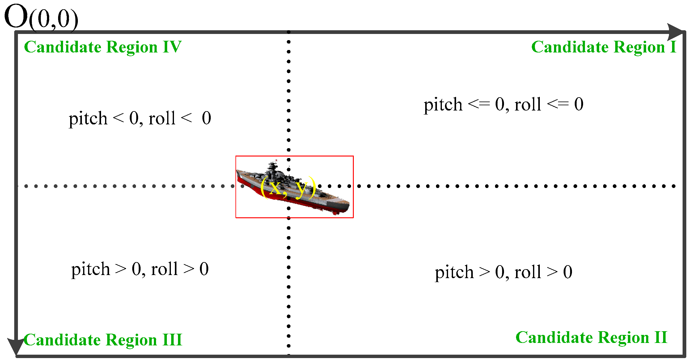
When the target vessel moves closer to the camera, the bounding box of imaging area gradually becomes larger and vice versa. Suppose that the bounding box center of the current target vessel is at (x, y) coordinate of the image, x and y divide the whole image into four quadrants, and each quadrant is a candidate region. We present four possible situations in Figure 5, while considering the pitching and rolling attitude of the ego vessel at the present moment.

3.3.2. Long-Term Cues

It is well known that the condition of a vessel on the sea is much more complex than that of vehicles and pedestrians on the ground due to the influence of environmental factors, such as waves, wind, and ocean currents. The camera also moves with the movement of the ego vessel, such as swing (surge, sway, and heave) and rotating (roll, pitch, and yaw), which cause the target to be temporarily lost from the camera scene. These dramatic changes on sea surface require the re-identification of the same vessel from adjacent frames or even across some frames according to their similarity measurements as the long-term cues.
The MDNet structure proposed in [22] was employed here, and a dataset with more than 500 vessels and nearly 150,000 images, named Ship-ReID, was constructed. We found the optimal mapping from image space to feature space after training on it. Suppose that inputs are triplet units { <   a , p , n   > } , indicating the anchor image, positive image, and negative image, respectively. <   a , p   > is a positive pair belonging to the same vessel, while <   a , n   > is the negative pair from different vessels. We used the normalized cosine similarity between the feature vector to measure the distance, such as D a , p and D a , n , and guided the network to train in the direction of pushing positive and negative samples away. We ensured that the distance between positive samples was very close by means of the improved triplet loss, as follows:
( a , p , n ) = N [ D a , p + m a x ( D a , p D a , n + λ , 0 ) ]
where λ is the pre-set threshold parameter.

3.3.3. Data Association and Fusion Method

As introduced in [42], we adopted heuristic simulated annealing to solve the assignment problem during the data association stage [43]. Assuming that we have D detectors and T tracklets waiting to match at time k , and D = { d 1 , d 2 , , d D } , T = { t 1 , t 2 , , t T } , G ( k ) is the adaptive gate association set, and ( k ) is the tracking gate set consisting of the rectangular region generated by the coordination predicted by MM filter trackers. Subsequently, the association cost matrix between the i -th tractlet’s predictions t ^ i ( k ) and the j -th detectors d j ( k ) could be defined as
C ( k ) ( i , j ) = { c ( k ) ( t ^ i , d j ) , i f   d j ( k ) G i ( k )   o r   d j ( k )   G i ( k ) ,       otherwise
where c ( t ^ i , d j ) is the hybrid affinity metric of association at time k when the j -th detector falls into the correlation gate corresponding to the prediction coordinate of the i -th tracklet, which can be calculated as
c ( k ) ( t ^ i , d j ) = ( 1   A ) m o t i o n ( k ) ( t ^ i ( k ) , d j ( k ) ) + A a p p e a r ( k ) ( t ^ i ( k ) , d j ( k ) )
where the weight coefficient is denoted as A , which is depicted by the attitude of the ego vessel. Equation (18) demonstrates that, as the pitch and roll of the hull increase, the weight of the appearance is enhanced, and vice versa.
A = [ ( p ( k ) ) 2 + ( r ( k ) ) 2 ] 1 / 2 λ [ ( p m a x ) 2 + ( r m a x ) 2 ] 1 / 2
where p , r is the dynamic pitch and roll at time k, which can be obtained from real-time measurement of the ego vessel’s electric compass or IMU; p m a x , r m a x represent the maximum range of pitch and roll, which are determined by the intrinsic characteristics of the hull, which can be obtained from prior measurement; and, λ is a hyper parameter.
a p p e a r ( t ^ i , d j ) is the measurement of appearance similarity between t ^ i and d j , and m o t i o n ( t ^ i , d j ) represents their measurements of motion similarity that were obtained by calculating the negative logarithm of the intersection-of-union ratio:
m o t i o n ( t ^ i ( k ) , d j ( k ) ) = l o g ( I n t e r s e c t i o n ( t ^ i ( k ) , d j ( k ) ) U n i o n ( t ^ i ( k ) , d j ( k ) ) )

3.4. The Proposed M3C Tracking by Detection

In this section, an end-to-end and real-time tracking by detection pipeline is presented, for which the tracklet initiation and termination conditions were both determined by a continuous three-frame method, as described in Algorithm 1:
Algorithm 1: The proposed M3C tracking by detection
Inputs: The sequential frames of surrounding vessels S , pre-trained GRU model M g r u , Darknet53 model M d 53 , Ship-Reid model M r e i d , and periodic attitude data A of the ego vessel
Initialization: T , A m a x , ( v k ) c o u n t = 0 , ( t i ) c o u n t = 0
Outputs: Continuous tracklets T = { t i } i = 1 M of surrounding vessels
Procedure:
  foreach frame at current time t
    detect all potential vessels V = { v k } k = 1 N from the t frame using M d 53
    foreach tracklet of vessel  // Association gate generated from prior time
      Predict the kinematic track gate from MM filter from time t 1
      & adaptive association gate of appearance
    endfor
    MC data association using simulated annealing algorithm
    foreach pair of matched detection and tracklet
      tracklet update by MM filter
    endfor
    foreach detection vessel v k not associated with any tracklets in T
       ( v k ) c o u n t + +
      if ( v k ) c o u n t > = 3   //Three-frame tracklet initiation
        initialize a new tracklet t
         T = { t }
      end
    endfor
    foreach vessel tracklet t i not associated with any detection in V
       ( t i ) c o u n t + +
      tracklet extrapolation
      if ( v k ) c o u n t > = λ m a x   // Extrapolation times exceeding the pre-set value λ m a x
        terminate the tracklet t i
         T = T { t i }
    end
  endfor
  endfor  //reach the end of the video sequence

4. Experiment and Results Analysis

4.1. Experimental Setup

4.1.1. Datasets

We performed extensive experiments on SMD [1] and the PETS 2016 maritime dataset [6] to evaluate performance of the proposed M3C. The detector was pretrained on a Marvel vessel image dataset by the offline method [44].
SMD contains 51 annotated video fragments, 40 onshore videos, and 11 onboard videos. We estimated the approximate range of roll and pitch of the ego vessel from horizon ground truths (GTs). The PETS 2016 maritime dataset includes 20 RGB video fragments that were captured by four digital pan-tilt-zoom (PTZ) cameras, three of which were at the side and one at the stern. Two skiff boats and two fish boats as the supplementary target vessels performed behaviors, such as speeding up, loitering, moving around the ego vessel, and so on. The collected the Marvel vessel image dataset that consisted of more than 140,000 vessel images. It was divided into 26 superclasses, drawing from the www.shipspotting.com website of online vessel photos and trackers. We resized the image to 608 × 608 pixels and manually labeled all of the selected pictures as belonging to five superclasses, which were tug ship, container, fish boat, skiff boat, and passenger ship.

4.1.2. Implementation Details

We used an i7-8700K CPU with 32 GB of memory and dual NVIDIA Titan RTX GPU with a Pytorch deep learning framework to implement our algorithm. We devised the detector based on the state-of-the-art YOLOv3, as mentioned in the previous section. The size of prior anchors is list in Table 1.
We used GRU with 128 units for the vessel’s maneuverability discrimination and trained the model while using Adam with a dropout of 0.2 for regularization and with a learning rate of 0.001. Due to the lack of adequate vessel tracklets or video galleries for training, it was pretrained by the public AIS dataset [45], and was then fine-tuned on the training set partitioned from SMD and PETS 2016.

4.2. Performance Evaluation

4.2.1. Evaluation Metric

The evaluation was carried out according to the standard root mean square error (RMSE)/mean absolute deviation (MAE) and CLEAR MOT metrics that were proposed in [46], and a brief description of each metric is listed below:
MOTA (↑): multi-object tracking accuracy, as calculated by the following formula:
M O T A = 1 t ( N F N ( t ) + N F P ( t ) + N I D S ( t ) ) t N G T ( t )
where N F N ( t ) , N F P ( t ) , and N I D S ( t ) are the number of false negatives, false positives, and IDS in the t frame index; and, N G T ( t ) represents the number of ground truth targets.
MOTP (↑): multi-object tracking precision, as calculated by the following formula:
M O T P = i , t d i ( t ) t ( N T P ( t ) + N I D S ( t ) )
where N T P ( t ) is the number of true positives in the t frame index and d i ( t ) represents the bounding box overlap of the i-th target.
RMSE (↓): root-mean-square error; MAE (↓): mean absolute deviation; MT (↑): mostly tracked targets; ML (↓): mostly lost targets; FN (↓): total number of false negatives; FP (↓): total number of false positives; IDS (↓): identity switches; FPS (↑): frames per second; and, mAP (↑): mean average precision. The colored arrow after each metric index indicates whether the value of increasing (↑) or decreasing (↓) is beneficial. MOTP and MOTA lie in the range of [0,100%], with the best value being 100%.

4.2.2. Qualitative Results

For the sake of fairness, performance comparison was separately carried out according to onshore or onboard datasets, because the results of some trackers can be biased due to camera motion. We discuss the comparison with state-of-the-art tracking methods, such as the framework of Markov decision process (MDP) [47], the combination of Kalman filter and Hungarian assignment algorithm (SORT) [48], the kernel correlation filter method (KCF) [49], the combination of Kalman filter and Kuhn-Munkres (POI) [50], SORT with deep association metric (DeepSORT) [19], and candidate selection combined with re-identification (MOTDT) [51].
The M3C pipeline obtained a 2.5% increase and a 33.5% decrease in MOTA and IDS as compared with the second best onshore dataset, as shown in Table 2. As far as the onboard dataset, the corresponding figures were 3% and 30.6%, and ML was also the lowest. In addition, on both onshore and onboard datasets, FPS was more than 10 in both scenarios, which indicated that real-time performance was obtained.

4.2.3. Visual Tracking Results

We present the visual tracking results of some videos to illustrate the performance of our proposed M3C framework intuitively.
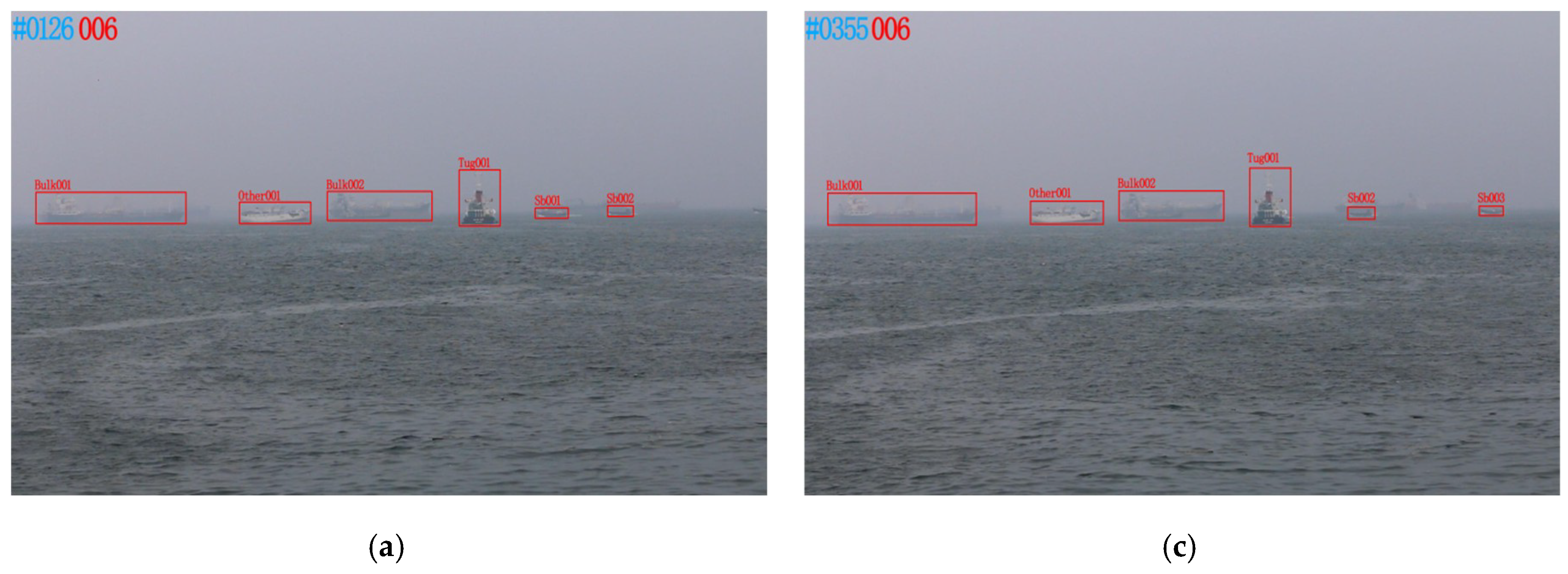
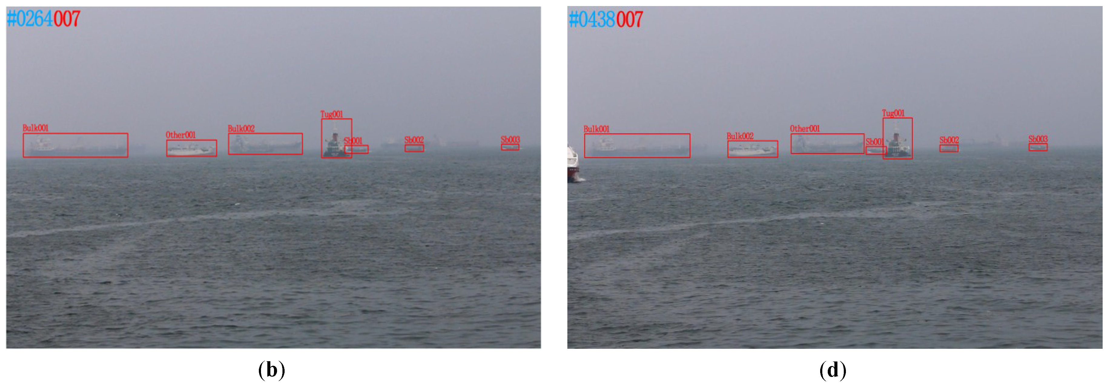
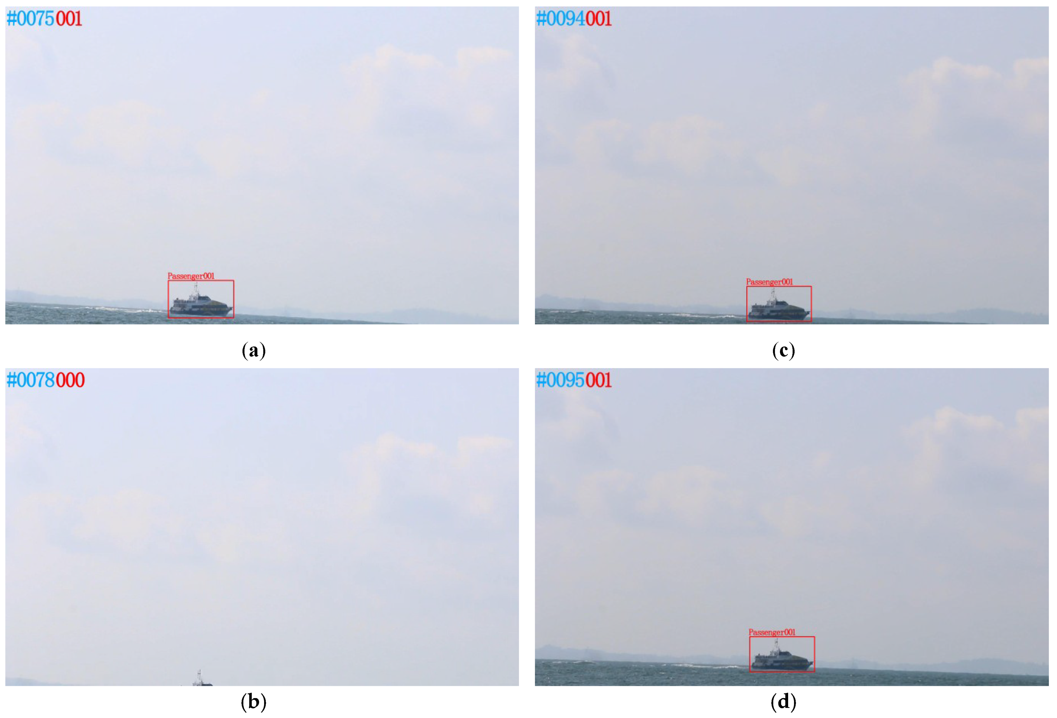
In Figure 6 and Figure 7, we show the tracking robustness of a reappearing vessel after being lost for a short time Figure 7b, and even complete occlusion Figure 6b, for which our proposed Ship-ReID worked well as the long term cue.

4.3. Ablation Study and Analysis

4.3.1. Effect of Multimodel Fusion Filter

In this scheme, we considered three different motion scenarios of the target vessel, including a straight line with constant velocity motion, acceleration, and turning motion. We conducted an ablation experiment by replacing MM with a single Kalman filter ( CV ) and interactive multiple models (IMM) [52] while considering the CA , CV , and CM model by keeping other conditions unchanged. RMSE and MAE were used as the evaluation indicators, respectively. Table 3 shows the comparison results.
IMM did not perform better than the single CV model with a Kalman filter when no maneuver occurred and was even worse than the latter, because of the possible delay of model transfers, as can be seen in Table 3. The proposed MM filter overcame this very well, and RMSE and MAE both increased by 30% in the three common motion scenarios.

4.3.2. Effect of Detector

As illustrated in Table 4, the detector built on YOLOv3 with Darknet53 as the backbone increased mAP by nearly 40% when compared with SSD, and FPS was five times higher than that of faster R-CNN. It was a good compromise between mAP and FPS, and both of them were equally critical for improving tracking performance. These experiments showed that the quality of the detection algorithm has significant influence on multi target tracking performance.

4.3.3. Effect of Multicue Data Association

It can be observed from Table 5 that the M3C pipeline obtained the highest value of MOTA, which is one of the most important indicators of multitarget tracking. These data lead us to the conclusion that combining the motion features with appearance features can effectively improve the tracking accuracy.
By combining deep feature extraction and a traditional kinematic filtering algorithm, the proposed M3C approach strikes a balance between tracking accuracy and speed and improves tracking accuracy while guaranteeing real-time performance, as discussed previously.

5. Conclusions

We proposed a novel tracking by detection approach integrating MM and MC to detect and track surrounding vessels of USVs at sea in this paper. MM was used to solve the problem of unstable tracking of a maneuvering target in the traditional single-model Kalman tracker (such as the CV model). MC combines the attitude of the ego vessel and the appearance of the target vessels to solve the problem of frequent IDS that is caused by motion blurring and occlusion. Experiments have demonstrated its efficiency and robustness and it achieved real-time performance. In the future, we plan to focus on the following two directions. First, we will construct a more complete Ship-ReID dataset and optimize the network framework and algorithm. Second, we intend to integrate Ship-ReID with a convolutional neural network of the detector and to co-train them in a unified network, so as to further improve the real-time performance.

Author Contributions

D.Q. proposed the M3C method, designed the experiments, and was responsible for writing the paper. G.L. was in charge of the literature search and drafted this manuscript. Q.Z. and F.D. made substantial contributions to the ship image acquisition and data analysis. J.Z. and G.W. performed the experiments and contributed to modifying the paper.

Funding

This paper was sponsored by the National Science Foundation of China (61202370); the Qinglan project and advanced study and research (2018GRF016) of Jiangsu Province; the project of the Jiangsu maritime safety administration (HTJ2019042); the scientific research fund of the Hunan Provincial education department (15C1241); the project of the Qianfan team, innovation fund, and the collaborative innovation center of shipping big data application (2017KJZD-02,KJCX1809), JMI; and the 13th five-year plan of educational science in Jiangsu Province (D/2016/03/17).

Conflicts of Interest

The authors declare no conflict of interest.

References

  1. Prasad, D.K.; Rajan, D.; Rachmawati, L.; Rajabally, E.; Quek, C. Video Processing from Electro-Optical Sensors for Object Detection and Tracking in a Maritime Environment: A Survey. IEEE Trans. Intell. Transp. Syst. 2017, 18, 1993–2016. [Google Scholar] [CrossRef]
  2. Bloisi, D.; Iocchi, L. ARGOS—A video surveillance system for boat traffic monitoring in venice. Int. J. Pattern Recognit. Artif. Intell. 2009, 23, 1477–1502. [Google Scholar] [CrossRef]
  3. Kang, Y.T.; Chen, W.J.; Zhu, D.Q.; Wang, J.H.; Xie, Q.M. Collision avoidance path planning for ships by particle swarm optimization. J. Mar. Sci. Technol. 2018, 26, 777–786. [Google Scholar]
  4. Dijk, J.; van der Stap, N.; van den Broek, B.; Pruim, R.; Schutte, K.; den Hollander, R.; van Opbroek, A.; Huizinga, W.; Wilmer, M. Maritime detection framework 2.0: A new approach of maritime target detection in electro-optical sensors. In Proceedings of the Electro-Optical and Infrared Systems: Technology and Applications XV, Berlin, Germany, 9 October 2018; Volume 10795, p. 1079507. [Google Scholar]
  5. Yazdi, M.; Bouwmans, T. New trends on moving object detection in video images captured by a moving camera: A survey. Comput. Sci. Rev. 2018, 28, 157–177. [Google Scholar] [CrossRef]
  6. Patino, L.; Nawaz, T.; Cane, T.; Ferryman, J. Pets 2016: Dataset and Challenge. In Proceedings of the IEEE Computer Society Conference on Computer Vision and Pattern Recognition Workshops (CVPR), Las Vegas, NV, USA, 1–26 June 2016; pp. 1–8. [Google Scholar]
  7. Girshick, R. Fast R-CNN. In Proceedings of the IEEE International Conference on Computer Vision (ICCV), Santiago, Chile, 7–13 December 2015; pp. 1440–1448. [Google Scholar]
  8. Ren, S.; He, K.; Girshick, R.; Sun, J. Faster R-CNN: Towards Real-Time Object Detection with Region Proposal Networks. IEEE Trans. Pattern Anal. Mach. Intell. 2017, 39, 1137–1149. [Google Scholar] [CrossRef] [PubMed] [Green Version]
  9. Dai, J.; Li, Y.; He, K.; Sun, J. R-FCN: Object detection via region-based fully convolutional networks. In Proceedings of the Advances in Neural Information Processing Systems, Barcelona, Spain, 5–10 December 2016; pp. 379–387. [Google Scholar]
  10. Liu, W.; Anguelov, D.; Erhan, D.; Szegedy, C.; Reed, S.; Fu, C.Y.; Berg, A.C. SSD: Single shot multibox detector. In Proceedings of the Computer Vision—ECCV 2016, Amsterdam, The Netherlands, 8–16 October 2016; Lecture Notes in Computer Science. pp. 21–37. [Google Scholar]
  11. Redmon, J.; Farhadi, A. Yolov3: An Incremental Improvement. arXiv 2018, arXiv:1804.02767. [Google Scholar]
  12. Kong, T.; Sun, F.; Liu, H.; Shi, J. FoveaBox: Beyond Anchor-based Object Detector. arXiv 2019, arXiv:1904.03797. [Google Scholar]
  13. Zhu, C.; He, Y.; Savvides, M. Feature Selective Anchor-Free Module for Single-Shot Object Detection. arXiv 2019, arXiv:1903.00621. [Google Scholar]
  14. Tonissen, S.M.; Evans, R.J. Performance of dynamic programming techniques for track-before-detect. IEEE Trans. Aerosp. Electron. Syst. 1996, 32, 1440–1451. [Google Scholar] [CrossRef]
  15. Kieritz, H.; Hübner, W.; Arens, M. Joint detection and online multi-object tracking. In Proceedings of the IEEE Computer Society Conference on Computer Vision and Pattern Recognition Workshops (CVPRW), Salt Lake City, UT, USA, 18–22 June 2018; pp. 1540–15408. [Google Scholar]
  16. Gordon, D.; Farhadi, A.; Fox, D. Re3: Real-time recurrent regression networks for visual tracking of generic objects. IEEE Robot. Autom. Lett. 2018, 3, 788–795. [Google Scholar] [CrossRef]
  17. Bae, S.H.; Yoon, K.J. Confidence-Based Data Association and Discriminative Deep Appearance Learning for Robust Online Multi-Object Tracking. IEEE Trans. Pattern Anal. Mach. Intell. 2018, 40, 595–610. [Google Scholar] [CrossRef] [PubMed]
  18. Arandjelović, O. Automatic vehicle tracking and recognition from aerial image sequences. In Proceedings of the 12th IEEE International Conference on Advanced Video and Signal Based Surveillance (AVSS), Karlsruhe, Germany, 25–28 August 2015; pp. 1–6. [Google Scholar]
  19. Wojke, N.; Bewley, A. Deep cosine metric learning for person re-identification. In Proceedings of the 2018 IEEE Winter Conference on Applications of Computer Vision (WACV), Lake Tahoe, NV, USA, 12–15 March 2018; pp. 748–756. [Google Scholar]
  20. Yang, X.; Tang, Y.; Wang, N.; Song, B.; Gao, X. An End-to-End Noise-Weakened Person Re-Identification and Tracking with Adaptive Partial Information. IEEE Access 2019, 7, 20984–20995. [Google Scholar] [CrossRef]
  21. Zhao, D.; Fu, H.; Xiao, L.; Wu, T.; Dai, B. Multi-object tracking with correlation filter for autonomous vehicle. Sensors 2018, 18, 2004. [Google Scholar] [CrossRef] [PubMed]
  22. Liu, H.; Tian, Y.; Wang, Y.; Pang, L.; Huang, T. Deep Relative Distance Learning: Tell the Difference between Similar Vehicles. In Proceedings of the IEEE Computer Society Conference on Computer Vision and Pattern Recognition (CVPR), Las Vegas, NV, USA, 27–30 June 2016; pp. 2167–2175. [Google Scholar]
  23. Fefilatyev, S.; Goldgof, D.; Shreve, M.; Lembke, C. Detection and tracking of ships in open sea with rapidly moving buoy-mounted camera system. Ocean Eng. 2012, 54, 1–12. [Google Scholar] [CrossRef]
  24. Jeong, C.Y.; Yang, H.S.; Moon, K.D. Fast horizon detection in maritime images using region-of-interest. Int. J. Distrib. Sens. Networks 2018, 14. [Google Scholar] [CrossRef]
  25. Zhang, Y.; Li, Q.Z.; Zang, F.N. Ship detection for visual maritime surveillance from non-stationary platforms. Ocean Eng. 2017, 141, 53–63. [Google Scholar] [CrossRef]
  26. Sun, Y.; Fu, L. Coarse-fine-stitched: A robust maritime horizon line detection method for unmanned surface vehicle applications. Sensors 2018, 18, 2825. [Google Scholar] [CrossRef]
  27. Bovcon, B.; Perš, J.; Kristan, M. Stereo obstacle detection for unmanned surface vehicles by IMU-assisted semantic segmentation. Rob. Auton. Syst. 2018, 104, 1–13. [Google Scholar] [CrossRef] [Green Version]
  28. Cane, T.; Ferryman, J. Evaluating deep semantic segmentation networks for object detection in maritime surveillance. In Proceedings of the 15th IEEE International Conference on Advanced Video and Signal-Based Surveillance (AVSS), Auckland, New Zealand, 27–30 November 2018; pp. 1–6. [Google Scholar]
  29. Kim, K.; Hong, S.; Choi, B.; Kim, E. Probabilistic Ship Detection and Classification Using Deep Learning. Appl. Sci. 2018, 8, 936. [Google Scholar] [CrossRef]
  30. Marié, V.; Béchar, I.; Bouchara, F. Real-time maritime situation awareness based on deep learning with dynamic anchors. In Proceedings of the 15th IEEE International Conference on Advanced Video and Signal-Based Surveillance (AVSS), Auckland, New Zealand, 27–30 November 2018; pp. 1–6. [Google Scholar]
  31. Cao, X.; Gao, S.; Chen, L.; Wang, Y. Ship recognition method combined with image segmentation and deep learning feature extraction in video surveillance. Multimed. Tools Appl. 2019, 1–16. [Google Scholar] [CrossRef]
  32. Leclerc, M.; Tharmarasa, R.; Florea, M.C.; Boury-Brisset, A.C.; Kirubarajan, T.; Duclos-Hindié, N. Ship Classification Using Deep Learning Techniques for Maritime Target Tracking. In Proceedings of the 2018 21st International Conference on Information Fusion (FUSION), Cambridge, UK, 10–13 July 2018; pp. 737–744. [Google Scholar]
  33. Kejriwal, L.; Singh, I. A Hybrid Filtering Approach of Digital Video Stabilization for UAV Using Kalman and Low Pass Filter. Procedia Comput. Sci. 2016, 93, 359–366. [Google Scholar] [CrossRef] [Green Version]
  34. Best, R.A.; Norton, J.P. A new model and efficient tracker for a target with curvilinear motion. IEEE Trans. Aerosp. Electron. Syst. 1997, 33, 1030–1037. [Google Scholar] [CrossRef]
  35. Perera, L.P.; Oliveira, P.; Guedes Soares, C. Maritime Traffic Monitoring Based on Vessel Detection, Tracking, State Estimation, and Trajectory Prediction. IEEE Trans. Intell. Transp. Syst. 2012, 13, 1188–1200. [Google Scholar] [CrossRef]
  36. Li, J.; Dai, B.; Li, X.; Xu, X.; Liu, D. A Dynamic Bayesian Network for Vehicle Maneuver Prediction in Highway Driving Scenarios: Framework and Verification. Electronics 2019, 8, 40. [Google Scholar] [CrossRef]
  37. Hochreiter, S.; Schmidhuber, J. Long Short-Term Memory. Neural Comput. 1997, 9, 1735–1780. [Google Scholar] [CrossRef] [PubMed]
  38. Cho, K.; van Merrienboer, B.; Gulcehre, C.; Bahdanau, D.; Bougares, F.; Schwenk, H.; Bengio, Y. Learning Phrase Representations using RNN Encoder–Decoder for Statistical Machine Translation. In Proceedings of the 2014 Conference on Empirical Methods in Natural Language Processing (EMNLP), Doha, Qatar, 25–29 October 2014; pp. 1724–1734. [Google Scholar]
  39. Bar-Shalom, Y.; Blackman, S.S.; Fitzgerald, R.J. Dimensionless score function for multiple hypothesis tracking. IEEE Trans. Aerosp. Electron. Syst. 2007, 43, 392–400. [Google Scholar] [CrossRef]
  40. Hoiem, D.; Efros, A.A.; Hebert, M. Putting objects in perspective. Int. J. Comput. Vis. 2008, 80, 3–15. [Google Scholar] [CrossRef]
  41. Richardson, E.; Peleg, S.; Werman, M. Scene geometry from moving objects. In Proceedings of the Advanced Video and Signal-based Surveillance (AVSS), Seoul, South Korea, 26–29 August 2014; pp. 13–18. [Google Scholar]
  42. Racine, V.; Hertzog, A.; Jouanneau, J.; Salamero, J.; Kervrann, C.; Sibarita, J. Multiple-Target Tracking of 3D Fluorescent Objects Based on Simulated Annealing. In Proceedings of the 3rd IEEE International Symposium on Biomedical Imaging: Nano to Macro, Arlington, VA, USA, 6–9 April 2006; pp. 1020–1023. [Google Scholar]
  43. Osman, I.H. Heuristics for the generalised assignment problem: Simulated annealing and tabu search approaches. OR Spektrum 1995, 17, 211–225. [Google Scholar] [CrossRef]
  44. Gundogdu, E.; Solmaz, B.; Yücesoy, V.; Koc, A. MARVEL: A large-scale image dataset for maritime vessels. In Proceedings of the Asian Conference on Computer Vision (ACCV), Taipei, Taiwan, 21–23 November 2016; pp. 165–180. [Google Scholar]
  45. Nguyen, D.; Vadaine, R.; Hajduch, G.; Garello, R.; Fablet, R. A multi-task deep learning architecture for maritime surveillance using AIS data streams. In Proceedings of the 2018 IEEE 5th International Conference on Data Science and Advanced Analytics (DSAA), Turin, Italy, 1–3 October 2018; pp. 331–340. [Google Scholar]
  46. Bernardin, K.; Stiefelhagen, R. Evaluating multiple object tracking performance: The clear mot metrics. Eurasip J. Image Video Proc. 2008, 2008, 246309. [Google Scholar] [CrossRef]
  47. Xiang, Y.; Alahi, A.; Savarese, S. Learning to track: Online multi-object tracking by decision making. In Proceedings of the 2015 IEEE International Conference on Computer Vision (ICCV), Santiago, Chile, 7–13 December 2015; pp. 4705–4713. [Google Scholar]
  48. Bewley, A.; Ge, Z.; Ott, L.; Ramos, F.; Upcroft, B. Simple online and realtime tracking. In Proceedings of the 2016 International Conference on Image Processing (ICIP), Phoenix, AZ, USA, 25–28 September 2016; pp. 3464–3468. [Google Scholar]
  49. Henriques, J.F.; Caseiro, R.; Martins, P.; Batista, J. High-speed tracking with kernelized correlation filters. IEEE Trans. Pattern Anal. Mach. Intell. 2014, 37, 583–596. [Google Scholar] [CrossRef]
  50. Yu, F.; Li, W.; Li, Q.; Liu, Y.; Shi, X.; Yan, J. POI: Multiple object tracking with high performance detection and appearance feature. In Proceedings of the European Conference on Computer Vision (ECCV), Amsterdam, The Netherlands, 8–16 October 2016; pp. 36–42. [Google Scholar]
  51. Chen, L.; Ai, H.; Zhuang, Z.; Shang, C. Real-Time Multiple People Tracking with Deeply Learned Candidate Selection and Person Re-Identification. In Proceedings of the 2018 IEEE International Conference on Multimedia and Expo (ICME), San Diego, CA, USA, 23–27 July 2018; pp. 1–6. [Google Scholar]
  52. Labbe, R.R. Kalman and Bayesian Filters in Python. 2018. Available online: https://github.com/rlabbe/Kalman-and-Bayesian-Filters-in-Python (accessed on 20 May 2019).
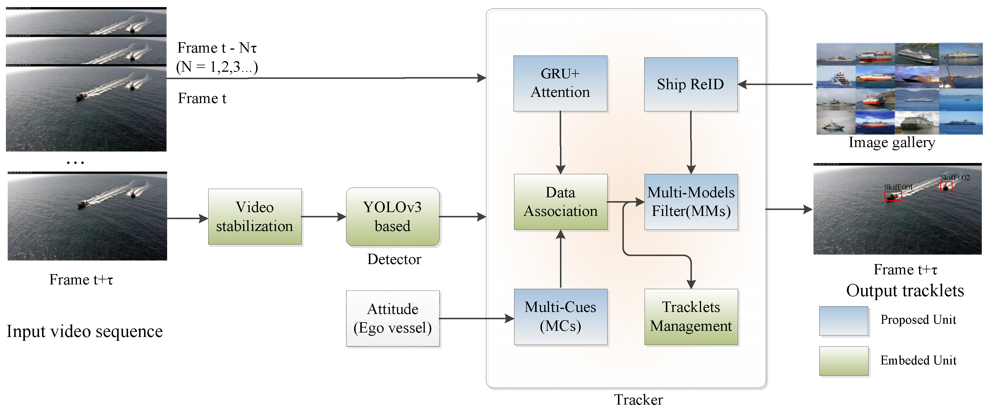
Figure 1. The architecture of our proposed M3C tracking by detection pipeline. It comprises eight modules, among which the video stabilization unit uses the algorithm introduced by [33]. We proposed the four blue units, and their interaction with the other three green units is discussed in detail later.
Electronics 08 00723 g001
Figure 2. Framework of the detector. Among them, Darknetconv2d_BN_Leaky (DBL) is the basic unit, which consists of a convolutional layer (conv), batch normalization, and a leaky rectified linear unit (ReLU).
Electronics 08 00723 g002
Figure 3. Typical structure of a gated recurrent unit (GRU) neural network. O t ( h t ) is the output at time t ; r t denotes the reset gate, which determines the combination of current input and historical memory information; and, z t is the update gate, which determines the proportion of memory left behind.
Electronics 08 00723 g003
Figure 4. The improved framework of the GRU encoder–decoder with attention. The attention model was embedded between encoders and decoders and learned the attention weights c t N τ   , , c t τ , c t , c t + τ via the fully-connected network (FC) and softmax with loss function, output vector of encoder h t N τ   , , h t τ , h t , h t + τ , and state vector of decoder s t ( N + 1 ) τ , s t N τ , , s t τ , s t as the attention model’s input sequence.
Electronics 08 00723 g004
Figure 5. Sketch map of adaptive association gate of appearance.
Electronics 08 00723 g005
Figure 6. Visual tracking results of video sequence (MVI_1448_VIS_Haze) with occlusion. Six vessels have been stably tracked in frame #0126 (a). Starting in frame #0264 (b), Sb001 was occluded by Tug001 until being completely occluded in frame #0355 (c) and then reappeared in frame #0370 until it was completely visible in frame #0438 as shown in (d).
Electronics 08 00723 g006aElectronics 08 00723 g006b
Figure 7. Visual tracking results of video sequence (MVI_0799_VIS_OB) with reappear after lost. In frame #0075 (a), a vessel has been stably tracked. Due to the rolling of the ego vessel, Passenger001 gradually disappeared from the camera scene in frame #0076 until frame #0078 (b), when it completely disappeared. Subsequently, it began to reappear in frame #0091 until frame #0094 (c), when it was completely visible. As shown in frame #0095 (d), the vessel was re-tracked steadily.
Electronics 08 00723 g007
Table 1. The feature map and prior anchors of Singapore Marine Dataset (SMD) and PETS 2016 maritime dataset. A total of nine anchors were used to generate bounding boxes, and the size of prior anchors was calculated by the k-means algorithm.
Feature Map19 × 1938 × 3876 × 76
Receptive FieldBigMediumSmall
Prior Anchors110 × 84176 × 93267 × 16635 × 6562 × 57107 × 3943 × 1938 × 3968 × 29
Table 2. Quantitative evaluation of different trackers on the two maritime datasets. We treated PETS 2016 as the onshore dataset considering a stationary large ship.
DatasetTrackerMOTA↑MOTP↑MT↑ML↓IDS↓FPS↑
SMD (onshore) + PETS 2016MDP30.3%71.3%13.2%38.4%4261
SORT59.8%79.6%25.4%22.7%63156
KCF70.3%80.2%37.8%22.3%38225
POI66.1%79.5%34.6%20.8%45310
M3C (Ours)72.8%80.4%37.4%21.2%25420
SMD (onboard)DeepSORT60.4%79.1%32.8%18.2%5636
MOTDT57.6%70.9%34.2%28.7%4923
M3C (Ours)63.4%74.6%26.217.9%3416
Table 3. Results of averaged RMSE and mean absolute deviation (MAE). SMD (onshore) and the PETS 2016 dataset were split into three different motion scenarios for the experiment, and a Kalman filter with a single constant velocity ( CV ) model was used as the benchmark.
Motion ScenariosAlgorithmAveraged RMSE (L2 Norm)Averaged MAE (L1 Norm)
X pos.Y pos.X pos.Y pos.
Straight line, constant velocityKalman ( CV )14.7116.0611.4714.53
IMM ( CV + CA + CM )15.1015.8712.0314.28
MM(Proposed)9.109.585.756.02
AccelerationKalman ( CV )27.7121.2925.3820.54
IMM ( CV + CA + CM )21.1718.2618.6715.88
MM(Proposed)13.9312.218.047.04
TurningKalman ( CV )20.9915.8519.5415.03
IMM ( CV + CA + CM )15.1013.1112.9310.98
MM (Proposed)12.449.568.806.67
Table 4. Detector performance in the ablation study. We replaced the detector with SSD and faster regions with CNN features (R-CNN), respectively, for these ablation experiments.
TrackerDetectormAPFPSAveraged RMSE (L2 Norm)Averaged MAE (L1 Norm)
X pos.Y pos.X pos.Y pos.
M3CSSD300 (Mobilenet)41.24620.2217.599.5416.37
YOLOv3 (Darknet53)57.9209.109.587.756.02
Faster R-CNN (Resnet50)59.148.946.398.445.83
Table 5. Results of the ablation study. multimodel (MM), single model (SM), and re-identification (ReID) denote appearance model, multimodel filter, single model filter, Ship-ReID, respectively.
TrackerDetectorMOTA↑MOTP↑MT↑ML↓IDS↓FPS↑
MMYOLOv346.2%44.5%12.9%43.2%7428
MM + AttentionYOLOv347.1%43.8%13.1%44.7%7332
SM+ReIDYOLOv359.8%64.5%21.4%23.6%6220
MM+ReID (M3C)YOLOv363.4%74.6%36.2%17.9%2416