1. Introduction
In the design of LQG controllers, due to the separation property between state estimation and control gain calculation, the design method of control law has received extensive attention from theorists and engineers. To date, a large number of problems in aerospace, aviation, industrial and socio-economic system have achieved satisfactory control effects under LQG framework, and many new methods have been deduced [
1,
2,
3]. However, all of these methods hold that the system’s actuators, sensors, etc. can work properly. When faults occur in the system, these methods not only fail to optimize system performance, but also destabilize the system and even put the system at risk. Therefore, it is thought to be of great theoretical and practical engineering significance to study the design method of the controller under LQG framework in the case of faults appearing in the system.
The LQG framework contains two aspects. On the one hand, the system dynamics are linear, while the disturbance acting on the process and the error affecting the measurements are white Gaussian noise. On the other hand, the performance index is quadratic in state and control with the form of convex function. The existing research results show that a linear state feedback control which makes the performance index of closed-loop system optimal and has the separation property can be determined under the condition that the system is normal. In the general case, the aging of the components, the varying of the environment and other unpredictable factors in the process of control will cause the system to deviate from normal operating conditions, and even cause system faults. The existing control algorithms are powerless. Faced with this challenge, this paper hopes to design a reliable controller. The reliable controller is thus a controller that can make a closed-loop system with an optimal performance index when the system is in normal conditions and can also make the closed-loop system with an acceptable performance under certain conditions when faults appear in the system. Notice that, when the system is under normal conditions, the controller is the conventional LQG optimal controller. A controller having this property is referred to as a reliable controller in this paper.
The primary role of a reliable controller is to handle system faults. Generally speaking, faults will inevitably occur in a system during its life cycle, such as the measurement deviation of sensor, the actuator stuck, etc. When these faults are reflected in the system model, they cannot be mathematically described by model parameters change, but by the model parameters jump in the high-dimensional discrete space. Essentially, each point in the discrete space corresponds to a model, and different control strategies are designed based on different models [
4,
5,
6]. If the fault model corresponding to any point in the discrete space is known, the number of models will have a dimension disaster, and it is impossible to refine the faults to different degrees to obtain all the models. A viable strategy is to build a cluster of models that traverse all possible faults as much as possible. The research results in this paper show that the reliable controller can be designed for a limited system model set. The controller tends to LQG optimal feedback control over time when the system is normal, and it can make the system have acceptable performance when the faults occur in the system.
A prerequisite for the reliable controller design is to approximate the various conditions of the system with a cluster of models which includes a normal model with no faults and several known fault models. The a priori information of the fault model is based on an understanding and mastery of history of the system, especially for systems that operate repeatedly in different cycles, such as aeronautical vehicles. There have been some methods for the problem of controller design with a model set that has multi-model control strategies [
7,
8]. These methods require that the controller is able to detect the fault model immediately. As system faults differ, the control laws matching different models are constantly switched according to the switching indicators, which often leads to strong jitter in the system at the switching point [
9,
10]. This is a hard switching method. Although it can make the system response faster, the jitter is unavoidable. In fact, a variety of methods that are accompanied by the development of sliding mode variable structure technology appear to solve the jitter.
In order to avoid the jitter, soft switching methods came into being [
11,
12]. In this paper, a soft switching among multiple models is realized by means of the dual adaptive control method. Since Feldbaum first proposed the dual control method for the autoregressive moving average (ARMA) model with unknown parameters, after more than half a century of research, it has been proved that dual control can optimize the system toward the desired target on one hand, and on the other hand, it can actively collect information and guarantee the unknown parameter estimation process [
13,
14,
15].
Based on the above analysis, the contribution in this paper is as follows: (1) It is assumed in this paper that the normal model and the possible fault models are known. LQG optimal control is applied for each model. By using the a posteriori probability of each model as the weight information, an MMRC is proposed; (2) It is the optimal LQG controller when the system is normal, and the controller performs reliably when faults occur in the system; (3) It neither needs to detect the fault model, nor needs to detect the fault time; (4) It implements a soft switching among the multiple models, which avoids the jitter caused by hard switching.
The remainder of this paper is organized as follows: the problem to be solved in this paper will be presented in
Section 2. The theoretical basis of MMRC will be established in
Section 3.
Section 4 illustrates the validity of the control algorithm through an example of the lateral-directional control system of an aircraft, and, finally, the conclusions will be offered in
Section 5.
2. Problem Statement
Consider the following discrete-time stochastic linear systems:
where
is an
n-dimensional vector of state,
is a
p-dimensional vector of output and
is an
m-dimensional vector of control input. The process noise
, observation noise
and initial condition
are mutually independent white Gaussian, whose statistics are
,
, and
.
,
and
are matrices of appropriate dimensions, and their variable quantities
represent the deviation of system components, actuators and sensors when the system is in operating mode
j,
. When
, it represents that the system is in normal mode and there is no fault, and the corresponding
. When
, it represents that the system is in different fault modes respectively, and, for any fault mode
corresponds to a set of determined values. In this paper, it is assumed that
are known a priori; that is, the model parameters corresponding to the mode
j are known, but which mode the system is in is unknown. In addition, the system can only be in one mode during the same stage, and, in different stages, the system mode is variable.
The performance index for the system is quadratic in the state and control
where
A and
B are positive semi-definite and positive definite symmetric matrices of appropriate dimensions, respectively.
Define the information set at time
k to be
The problem to be solved in this paper is to find a feedback control law
such that the expected performance index
of system (1) and (2) is minimized, namely,
Note that, if the process model parameters are completely known, the above control problem becomes the classical LQG control problem, for which there is already a mature solution. However, the problem solved in this paper is different from LQG, namely, the fault at current time is unknown and which fault is also unknown.
3. Reliable Controller Design
For the convenience of problem statement and notation, systems (1) and (2) can be rewritten as follows:
where
,
,
,
is the state of the system under mode
j, and
is the output.
Definition 1. When the system is in mode j, the state estimate based on real-time information set is can be obtained by the Kalman filter, [16]wherewith initial condition and . being the filter gain. Theorem 1. When the system is in mode j, the control law that minimizes performance index is given bywhere, for ,with the boundary condition . can be obtained from Definition 1. Proof of Theorem 1. Let the optimal cost-to-go of the operating mode
j at time
k be
According to the smoothing property of expectations and optimal theory of stochastic dynamic programming, we have
with the boundary condition
The solution to can be obtained by using dynamic programming. Let l denote the time. If (11) is true at the initial time , let it be true when . If it can be proved that it is true when , then the theorem is proved.
Substituting (16) into (17), according to the nature of trace and Definition 1, yields
Equation (
18) is quadratic in control
. Letting
, we can get the LQG optimal control
at time
,
where
is identical to (12). Substituting (19) into (18), then the optimal cost-to-go at the time
is given as
where
is identical to (11), and
is uncorrelated to control and state variables
Assume that at time
we have
According to (15), we can get
Substituting (20) into (21) by mathematical induction yields the following:
Similarly, letting
, we get the LQG optimal control
where
and (12) are identical. Substituting
into performance index
, we get
where
is identical to (14), and
is uncorrelated to control and state variables
This completes the proof. □
During the operation, the system may be in the normal mode, or switch back and forth among s fault modes. According to Theorem 1, each mode corresponds to an LQG optimal control. How to apply reliable control to the system based on LQG optimal control, the following theorem answers this question.
Theorem 2. The control law that minimizes the performance index of the system (1) and (2) at time k iswhere is the LQG optimal control law when the system is in mode j, is the a posteriori probability of mode j and satisfies the following recursive equation:wherewith the boundary condition . and are identical to (8) and (10), respectively. Proof of Theorem 2. According to the stability theorem of filter, it can be obtained that, when
, the limit of
is a constant matrix that is denoted as
. Let
i be the real system, for the non-real system
j,
, define
, according to (23), we have
Substituting (24), (25) and the boundary condition
into (26)
where
is replaced by its limit
. Taking the logarithm on both sides of (27), and, according to the nature of trace, we get
Since
i is a real system, we have
According to the ergodicity of the innovation sequence
it can be obtained that, when
,
For the non-real system
j, innovation
let
Substituting (31) and (32) into (30) yields
Since
and
are uncorrelated, according to (25), we get
Notice that
is a semi-positive matrix such that
holds if and only if
; then, we have
Substituting (29), (33) into (28), when
, we get
where
Since the right side of (34) is negative, when
where
. Then, we have
where
K is a constant. Therefore, when
, we have
, so we get
, since
=1, we get
.
At this time, the reliable control law = applied to the real system will tend to . This completes the proof. □
The above assumption of the boundary condition indicates that the reliable controller does not have any preference for the system modes at the initial time, which is the worst case from the viewpoint of probability, even though the reliable controller will still tend to the control law of the real system. Theorem 2 demonstrates the reliability of the controller, and also shows that MMRC implements a soft switching strategy.
Note that, when , , which is the a posteriori probability of true model i, tends to 1, while tends to 0. Suppose at some time unit k, ; it can be seen from (23) that and will no longer change. According to (22), it yields , namely, always equals the control law of model i. If the true model changes from i to j in the next stage, will not change to , which is referred to as “lock out”. The following theorem answers the question of how to unlock a posteriori probability.
Theorem 3. Assume that if the a posteriori probability of the system is locked out at time k, that is, the a posteriori probability of real system i, , and the a posteriori probabilities of non-real system j, , , then, through the following transformation,where , the a posteriori probability of the system after time k not only can be unlocked, but also does not affect the convergence. Proof of Theorem 3. According to (23), we have
Substituting (36) into (37), we get
where
is a constant. Let
=
, according to (24) and (25), we have
Comparing (38) with (27), similarly, we can prove that, when , if i is still real system, we have and then we can get ; if i becomes non-real system, then and . This completes the proof. □
One can see from Theorem 3 that is a constant, whose value only affects the convergence speed of the a posteriori probability and does not affect the convergence. That is, after the time k, no matter whether the system mode changes, the a posteriori probability of the real system will always tend to 1, and a posteriori probability of the non-real system will tend to 0.
4. Simulation Analysis
In summary, the design of the reliable controller can be implemented by the following algorithm:
Step 1: Calculate the Kalman gain offline according to (7)–(9).
Step 2: Calculate control gain offline according to (12)–(14).
Step 3: Set .
Step 4: Calculate and according to (10) and (6), respectively.
Step 5: Calculate according to (11).
Step 6: Calculate according to (23).
Step 7: Calculate control law according to (22), and apply this control to the system.
Step 8: Update according to (36).
Step 9: If , stop. Otherwise, set k := , go back to Step 4.
In order to illustrate the characteristics of the controller designed in this paper, an example of an aircraft lateral-directional control system [
17] is given as follows:
where system state
and control input
.
and
represent the bank angle, the sideslip angle, the body roll rate, and the body yaw rate, respectively.
and
denote the differential aileron and the rudder, which control the roll and yaw motion, respectively. The statistics for the process noise, observation noise and initial condition are
,
and
respectively where
is an identity matrix of
dimension.
Assume that the airspeed is excessive at fault time
due to the abnormality of the pitot tube system, and the process model parameters related to pitot tube are attenuated to 90% or 80%. That is, there are three potential operating modes in the system, i.e.,
, and the operation process of system is divided into two stages by
. Before
, we call it the first stage, and, after
we call it the second stage. It is further assumed that the real system is
in the first stage and in the second stage the real system is
. When the system is normal, i.e.,
, its model parameters are given as follows:
When the faults appear in the system, the relevant model parameters are 90% of the normal system, i.e.,
,
and 80% of the normal system, i.e.,
,
where
,
and
represent the elements of the second row and the first column, the second row and the second column in the matrix
G, and the second row and second column in the matrix
H respectively when the system is in mode
j. Note that we do not know which mode the system is in, and we do not know if the system mode is switched. We only know no matter which mode the system is in, its corresponding model is covered by the known model set
.
In this paper, two control strategies are used to implement example simulation. One is MMRC under the above conditions, the other is optimal control (OC) under the condition that the process model parameters are completely known. The performance index corresponding to OC should be the lower bound of the other controls. Simulation results are shown in
Figure 1,
Figure 2,
Figure 3,
Figure 4 and
Figure 5.
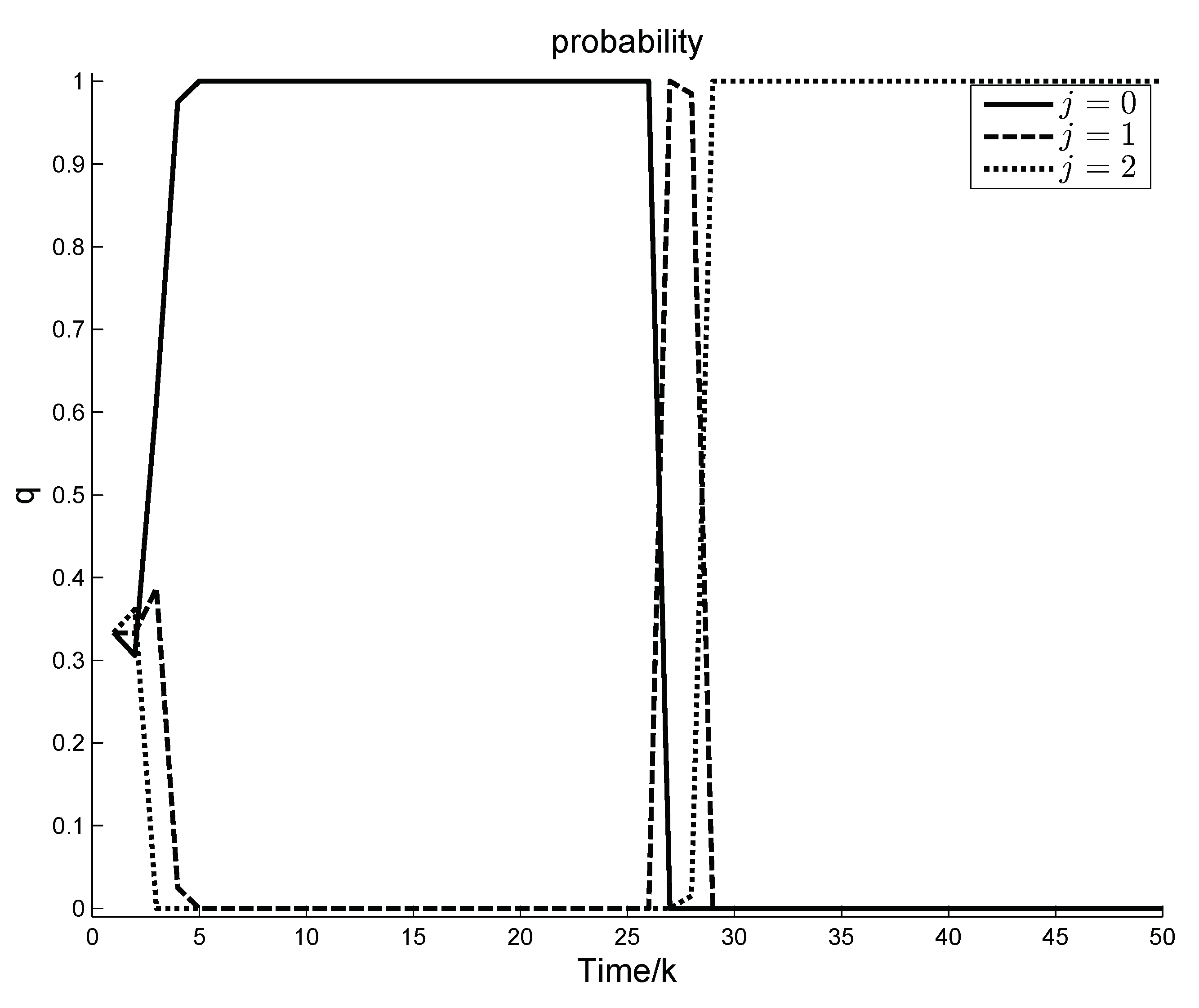
Figure 1 illustrates the variation curve of the a posteriori probabilities of different modes in
under MMRC.
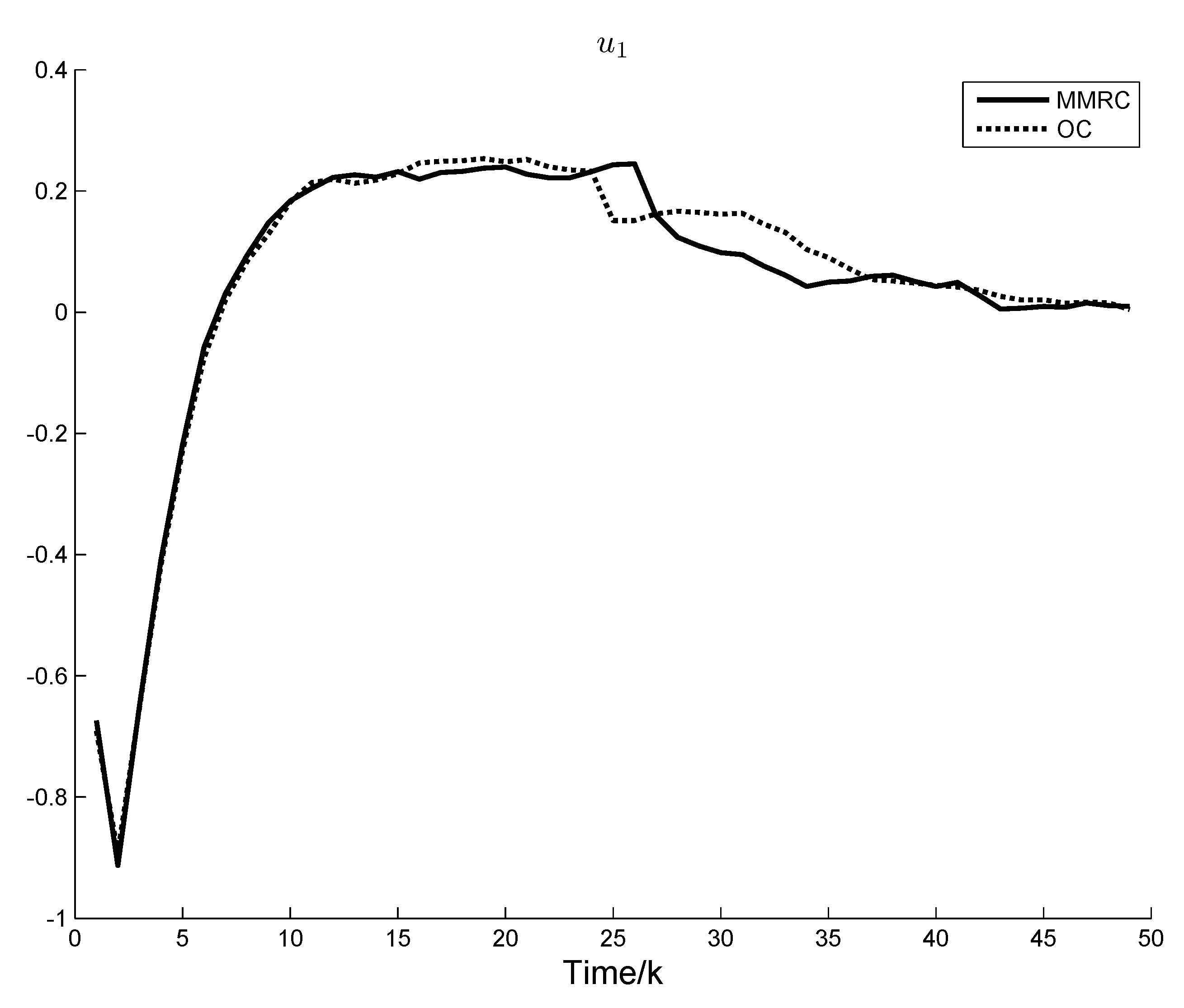
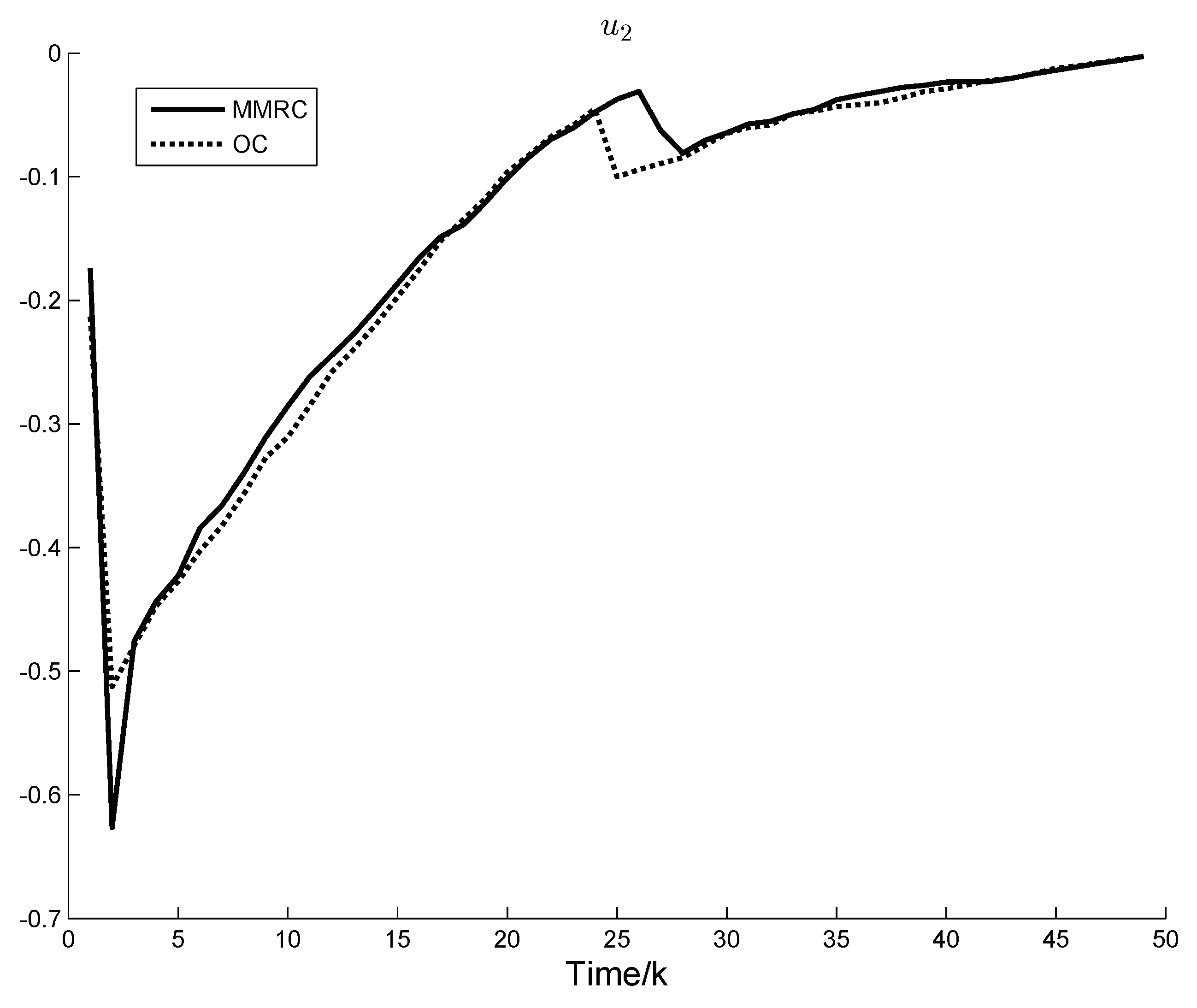
Figure 2 and
Figure 3 show the system control components under OC and MMRC, respectively.
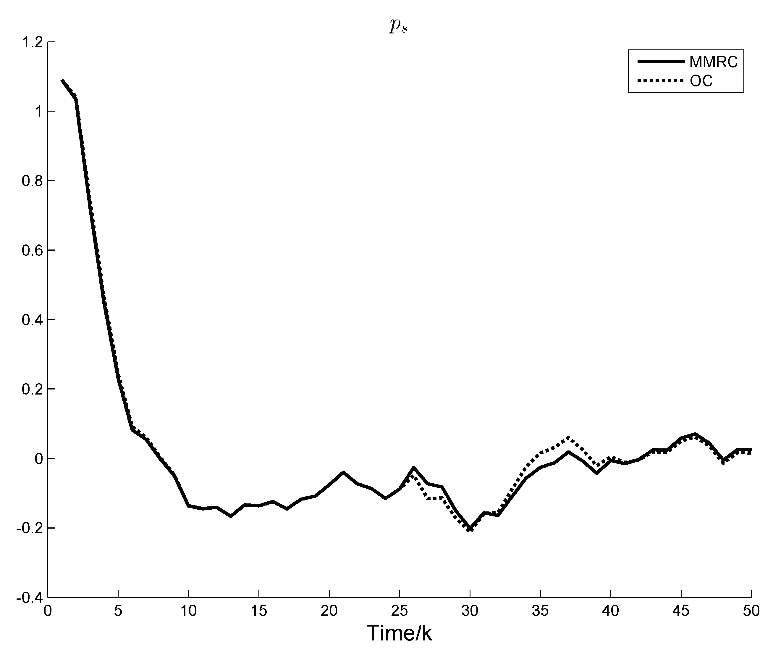
Figure 4 indicates the response curve of a representative system state. Performance index of the two control strategies are demonstrated in
Figure 5.
It is observed in
Figure 1 that in the above two stages the a posteriori probabilities of different system modes both have experienced change and stability. In the first stage, it is because the system is assumed with equal probability of
at the initial time, and, in the second stage, it is because a fault occurs in the system. As the system continuously obtains measurement results, the a posteriori probability of
tends to 1 and the a posteriori probabilities of
,
tend to 0 in the first stage, and in the second stage the a posteriori probability of
tends to 1 and the a posteriori probabilities of
,
tend to 0. It is noted that the change of the a posteriori probability of system is not 0 or 1, but varies between 0 and 1, which indicates that MMRC implements soft switching.
Figure 2 and
Figure 3 demonstrate that, in the first stage, MMRC follows closely OC except for the initial transient period. When fault occurs in the system in the second stage, a certain error lasts for a while, but then MMRC fluctuates around OC and eventually MMRC follows closely OC. It is observed in
Figure 4 that, in the first stage, there is only a slight difference in the state response curves under OC and MMRC, and, in the second stage, there is a deviation. However, the state response curve of MMRC finally follows closely that of OC in the control horizon.
Figure 5 demonstrates that only in the second stage is there a certain deviation between the performance index of MMRC and OC. These phenomena are due to two aspects. One is the switching of control law between multiple models, the other is the pursuit of control objective. Notice that it is an inevitable cost for MMRC.
5. Conclusions
In this paper, an MMRC, which is under the condition that the models are known, is given for controlling the variable fault system under LQG framework. The controller fuses the control law of each model by using their a posteriori probabilities as weight information. When the controller is in a deadlock state, a deadlock avoidance strategy is given and the convergence of the corresponding a posteriori probability is proved. The simulation results show that, when the system is normal, the controller is the optimal LQG control, and, when faults occur in the system, the controller is able to track optimal control quickly, which enables the performance of the fault system to closely follow the performance of that under OC. In addition, the controller neither needs to detect the system fault model, nor needs to detect the fault time. Soft switching strategy is implemented among the multiple models, which avoids the jitter caused by frequent hard switching to the system. If the system noise is non-Gaussian, extending the above algorithm to a non-Gaussian stochastic system will be future work.
