Article

Jet Features: Hardware-Friendly, Learned Convolutional Kernels for High-Speed Image Classification

Electrical and Computer Engineering, Brigham Young University, Provo, UT 84602, USA
*
Author to whom correspondence should be addressed.
Electronics 2019, 8(5), 588; https://doi.org/10.3390/electronics8050588
Submission received: 4 May 2019 / Revised: 21 May 2019 / Accepted: 22 May 2019 / Published: 27 May 2019

Abstract

:
This paper explores a set of learned convolutional kernels which we call Jet Features. Jet Features are efficient to compute in software, easy to implement in hardware and perform well on visual inspection tasks. Because Jet Features can be learned, they can be used in machine learning algorithms. Using Jet Features, we make significant improvements on our previous work, the Evolution Constructed Features (ECO Features) algorithm. Not only do we gain a 3.7× speedup in software without loosing any accuracy on the CIFAR-10 and MNIST datasets, but Jet Features also allow us to implement the algorithm in an FPGA using only a fraction of its resources. We hope to apply the benefits of Jet Features to Convolutional Neural Networks in the future.

1. Introduction

The field of computer vision has come a long way in solving the problem of image classification. Not too long ago, handcrafted convolutional kernels were a staple of all computer vision algorithms. With the advent of Convolutional Neural Networks (CNNs), however, handcrafted features have become the exception rather than the rule, and for good reason. CNNs have taken the field of computer vision to new heights by solving problems that used to be unapproachable or unthinkable. With deep learning, convolutional kernels can be learned from patterns seen in the data rather than pre-constructed by algorithm designers.
While CNNs are the most accurate solution to many computer vision tasks, they require many parameters and many calculations to achieve such accuracy. Efforts to reduce model size and operation complexity include binarization [1] and kernel separation [2]. In this work, we seek speed up image classification on simple tasks by leveraging some of the mathematical properties found in classic handcrafted kernels and applying them in a procedural way with machine learning. While this paper does not explore how these properties can be applied to CNNs using deep leering, we leave it for future work.
In this paper, we present Jet Features, a set of learned convolutional kernels. Convolutions with Jet Features are efficient to compute in both hardware and software. They take advantage of redundant calculations during convolutions and use only the simplest operations. We apply these features to our previous machine learning image classification algorithm, the Evolution Constructed Features (ECO Features) algorithm. We call this new version of the algorithm the Evolution Constructed Jet Features (ECO Jet Features) algorithm. It is accurate on simple image classification tasks, and can be efficiently run on embedded computer devices without the need for GPU acceleration. We specifically use Jet Features to allow the algorithm to be implemented in hardware.
We evaluate a software implementation and a hardware implementation of our algorithm to show the speed and compactness of the algorithm. Our hardware design is fully pipelined and gives visual inspection results as soon as an image reaches the end of the data pipeline. This hardware architecture was implemented on a Field Programmable Gate Array (FPGA), but could be integrated into a system on a chip in custom silicon, where it could perform at an even faster rate while using less power.
The original ECO Features algorithm [3,4] has been used in various industrial applications. Many of these applications require high-speed visual inspection, where speed is important but the identification task is fairly simple. In this work we speed up the ECO Features algorithm, allowing it to run 3.7 times faster in a software implementation, while maintaining the same level of accuracy on the MNIST and CIFAR-10 datasets. These improvements also make the algorithm suitable for full parallelization and pipelining in hardware, which runs over 70 times faster in an FPGA. The key innovations we make here are the development and use of Jet Features and development of a hardware architecture for our design.

Related Work

Convolutions are at the heart of almost all image processing techniques. FPGA platforms provide high parallelism, pipelining and distributed memory which has proved to be a good match for image convolutions and image processing in general [5,6,7,8,9]. In this work we use small, yet efficient, kernels for convolutions that use less memory then traditionally sized kernels.
Convolutions and other local image operators are commonly implemented by buffering an input steam of pixels, storing lines of the image [10,11,12,13]. Pixels from these buffers can be combined into sliding windows that form a neighborhood around a moving point from the image. This allows for image processing in local neighborhoods. Our work presented here explores the use of very small neighborhoods (2 × 1 and 1 × 2 windows) that are combined to efficiently process larger regions.
Efficient image processing on FPGAs has also been used to speed up image classification algorithms. Convolutional Neural Networks (CNNs) consist of sequences of convolutions that can be pipelined and performed in parallel with each other. While FPGAs can provide parallelism and pipelining to CNN algorithms, CNNs are traditionally trained with floating point values. FPGAs are not as well suited for floating point operations as GPUs and CPUs are. Courbariaux et al. explore the trade-offs in using fixed-point and low precision values over floating point values in deep learning [14]. They show that fixed-point and low precision values can be used in deep neural networks (DNNs) and achieve comparable accuracy as full precision floating point networks.
A variety of works have implemented CNNs in FPGAs with fixed-point values [15,16,17,18,19]. Not only do many FPGA implementations feature fixed-point values, but a class of CNNs focus on using low bit width values, called quantized neural networks [20,21,22].
Binarized Neural Networks (BNNs) are the most extreme form of quantized networks, where values are represented with a single bit for + 1 or 1 [1]. BNNs can utilize bitwise operations which make them well suited for FPGAs [23,24,25,26,27]. Xilinx Research Labs developed a framework for training BNNs and implementing them in and FPGA called FINN [28] with a follow called FINN-R for general fixed point precision [29]. Our method presented in this paper uses binarized weights similar to BNN, but uses full precision fixed-point pixel values and small convolutions. We also combine the results of our parallel image processing with a more traditional machine learning algorithm.

2. Jet Features

Jet Features are convolutional kernels with special structure that allow for efficient convolutions. They are meaningful features in the visual domain and allow for elegant hardware implementation. In fact, some of the most popular classical handcrafted convolutional kernels qualify as Jet Features, like the Gaussian, Sobel and Laplacian kernels. However, Jet Features are not handcrafted, they are learned features that leverage some of the intuition behind these classic kernels. Mathematically, they are related to multiscale local jets [30], which is reviewed in Section 2.2, but we introduce them here in a more informal manner.

2.1. Introduction to Jet Features

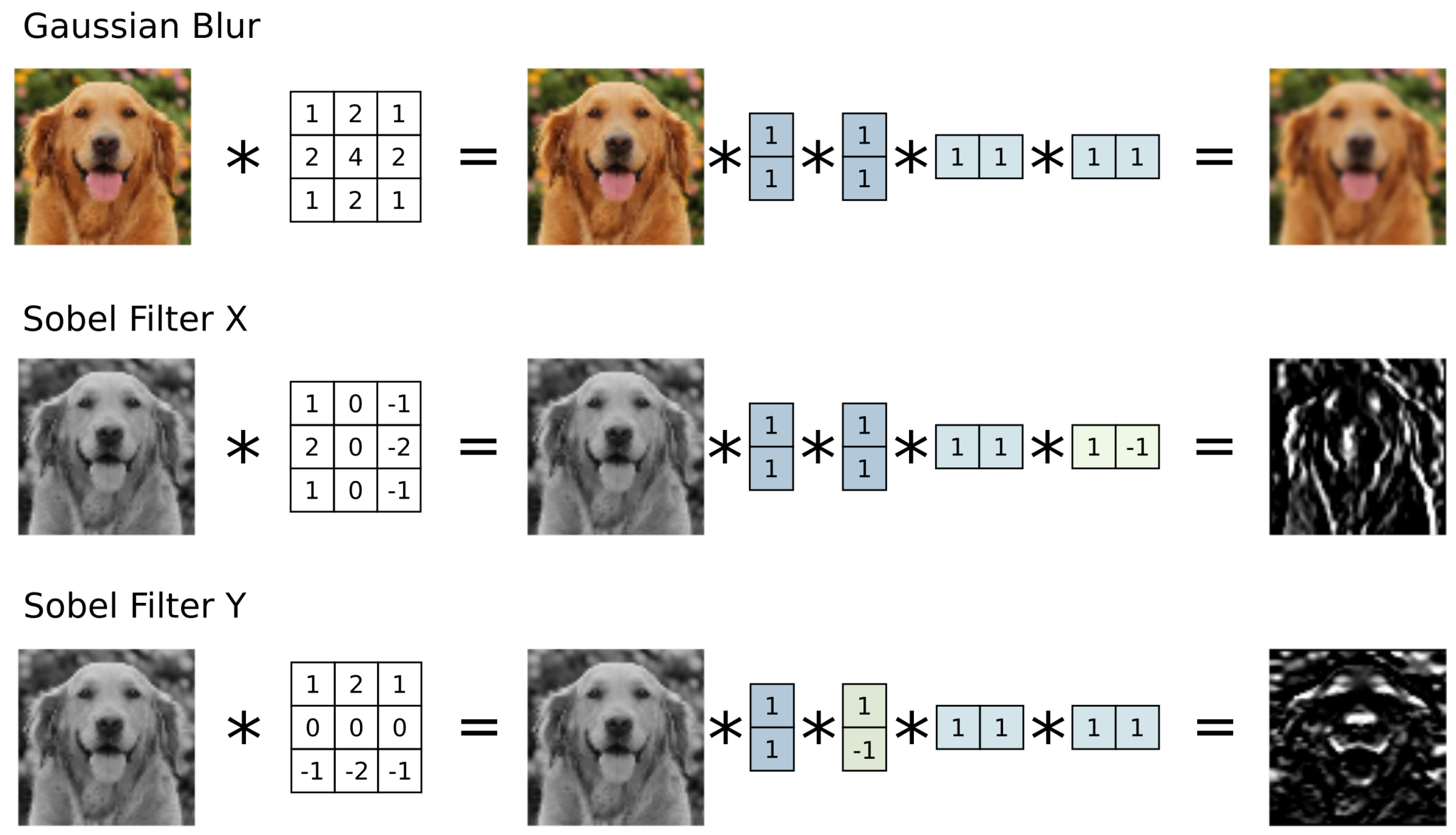
Jet Features are convolutional kernels that can be separated into a series of very small kernels. In general, separable kernels are kernels that perform the same operation as a series of convolutions with smaller kernels. Figure 1 shows an example of a 3 × 3 convolutional kernel that can be separated into a series of convolutions with a 3 × 1 kernel and a 1 × 3 kernel. Jet Features take separability to an extreme, being separated into the smallest meaningful sized kernels with only 2 elements. Specifically, all Jet Features can be separated into a series of convolutions with kernels from the set { [ 1 , 1 ] , [ 1 , 1 ] T , [ 1 , 1 ] and [ 1 , 1 ] T } , which are also shown in Figure 2. We will refer to these small kernels as the Jet Feature building blocks. Two of these kernels, [ 1 , 1 ] and [ 1 , 1 ] T , can be seen as blurring factors or scaling factors. We will refer to them as scaling factors. The other two kernels, [ 1 , 1 ] and [ 1 , 1 ] T , apply a difference between pixels in either the x or y direction and can be viewed as simple partial derivative operators. We will refer to them as partial derivative operators. All Jet Features are a series of convolutions with any number of these basic building blocks. With these building blocks, some of the most popular classic filters can be constructed. In Figure 3 we show how the Gaussian and Sobel filters can be broken down into Jet Feature building blocks.
It is important to note that the convolution operation is commutative and the order in which the Jet Feature building blocks are applied does not matter. Therefore, every Jet Feature is defined by the number of each building block it uses. For example, the 3 × 3 x-direction Sobel kernel can be defined as 1 x-direction and 2 y-direction scaling factors and 1 x-direction partial derivative operator (see Figure 3).

2.2. Multiscale Local Jets

We can more formally define a jet feature as an image transform that is selected from a multiscale local jet. All features for the algorithm are selected from the same multiscale local jet. Multiscale local jets were proposed by Florack et al. [30] as useful image representations that could capture both the scale and spatial information within an image. They have proven to be useful for various computer vision tasks such as feature matching, feature tracking, image classification and image compression [31,32,33]. Manzanera constructed a single unified system for several of these tasks using multiscale local jets and attributed its effectiveness to the fact that many other features are implcitly contained within a multiscale local jet [33]. Some of these popular features include the Gaussian blur, the Sobel operator and the Laplacian filter.
Multiscale local jets are a set of partial derivatives of a scale space of a function. Members of a multiscale local jet have been previously defined in [30,31,33] as
L x m y n σ ( A ) = A δ x m y n G σ ,
where A is an input image, δ x m y n is a differential operator to the degree of m with respect to x and degree n with respect to y and G σ is the Gaussian operator with a variance of σ . A multisacle local jet is the set of outputs L x m y n σ ( A ) for a given range of values for m, n and σ :
Λ x a y b [ σ c , σ d ] ( A ) = { L x 0 y 0 σ c ( A ) , , L x a y b σ d ( A ) } for all combinations between

3. The ECO Features Algorithm

We developed the original ECO Features algorithm in [3,4]. Its main purpose is to automatically construct good image features that could be used for classification. This eliminates the need for man experts to hand craft features for specific applications. This algorithm was developed as CNNs were gaining popularity, which solved similar problems [34]. We recognize that CNNs are able to achieve better accuracy than the ECO Features algorithm in most tasks, but ECO Features are smaller and generally less computationally expensive. In this paper we are interested in the effectiveness of Jet Features in the ECO Features algorithm. The impact of Jet Features are fairly straightforward to explore when working with the ECO Features algorithm. Exploration of Jet Features in CNNs is left for future work.
An ECO Feature is a series of image transforms performed back to back on an input image. Figure 4 shows an example of a hypothetical ECO Feature. Each transform in the feature can have a number of parameters that change the effects of the transform. The algorithm starts with a predetermined pool of transforms which are selected by the user. Table 1 shows the pool of transforms used in [4].
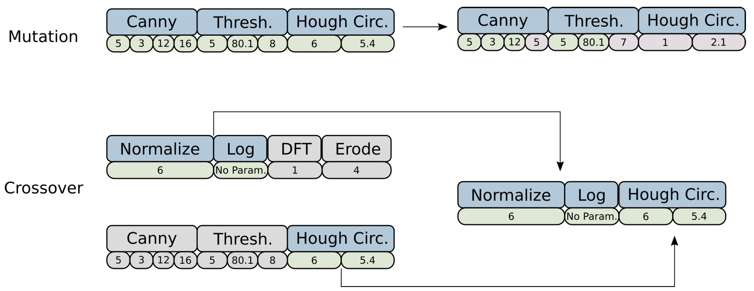
The genetic algorithm initially forms ECO Features by selecting a random series of transforms and randomly setting each of their parameters. The parameters of each transform are modified through the process of mutation in the genetic algorithm. New ordering of the transforms are also created as pairs of ECO Features are joined together in genetic crossover, where the first part of one series is spliced with the latter portion of a different series. A graphical representation of mutation and crossover are shown in Figure 5.
Each ECO Feature is paired with a classifier. An example is given in Figure 6. Originally, single perceptrons were used as the classifiers for each ECO Feature. Since perceptrons are only capable of binary classification, we seek to extend the algorithms capabilities to multiclass classification and we use a random forest [35] in this work. Inputs are fed through the ECO Feature transforms and the outputs are fed into the classifier. A hold set of images is then used to evaluate the accuracy of each ECO Feature. This accuracy is used as a fitness score when performing genetic selection in the genetic algorithm. ECO Features with high fitness scores are propagated to future rounds of evolution while weak ECO Features die off. The genetic algorithm continues until a single ECO Feature outperforms all others for a set number of consecutive generations. This ECO Feature is selected and saved while all others are discarded. The whole process is repeated for every ECO Feature produced by the genetic algorithm.
As the genetic algorithm selects ECO Features, they are combined to form an ensemble using a boosting algorithm. We use the SAMME [36] variation of AdaBoost [37] for multiclass classification. The boosting algorithm adjusts the weights of the dataset giving importance to harder examples after each ECO Feature is created. This leads to ECO Features tailored to certain aspects of dataset. Once the desired number of ECO Features have been constructed, they are combined into an ensemble. This ensemble predicts the class of new input images by passing the image through all of the ECO Feature learners, letting each one vote for which class should be predicted. Figure 7 depicts a complete ECO Features system.
Since the publications of [3,4] we have applied ECO Features to the problem of visual inspection where ECO Features were used to determine the maturity of date fruits [38]. This algorithm has also been used in industry to automate visual inspection for other processes.

4. The ECO Jet Features Algorithm

In this section we look at how Jet Features can be introduced into the ECO Features algorithm. We call this modified version the ECO Jet Features algorithm. This modification speeds up performance while maintaining accuracy on simple image classification. It was specifically designed to allow for easy implementation in hardware.

4.1. Jet Feature Selection

The ECO Jet Features algorithm uses a similar genetic algorithm to the one discussed in Section 3. Instead of selecting image transforms from a pool and combining them into a series, it simply uses a single Jet Feature. The amount of scaling and partial derivatives are the parameters that are tuned through evolution. These four parameters are bounded from 0 to a set maximum, forming the multiscale local jet, similar to Equation (2). We found that bounding the partial derivatives, δ x , δ y [ 0 , 2 ] , and scaling factors, σ x , σ y [ 0 , 6 ] , is effective at finding good features.
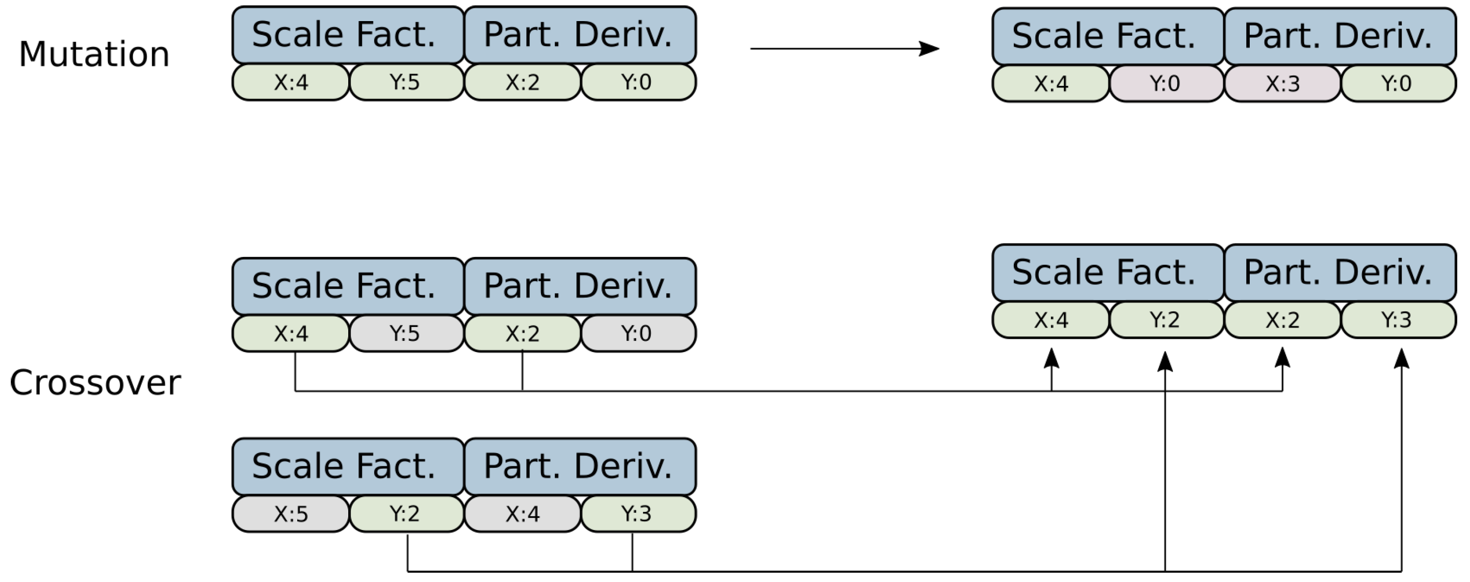
In order to accommodate the use of jet features, mutation and cross over are redefined. The four parameters of the jet feature, δ x , δ y , σ x and σ y , are treated like genes that make up the genome of the feature. During mutation, the values of these individual parameters are altered. During cross over, the genes of a child jet feature would each be copied from either the father or the mother genome. This selection is made randomly. This is illustrated in Figure 8.

4.2. Advantages in Software

The jet feature transformation can be calculated with a series of matrix shifts, additions and subtractions. Since the elements of the bases kernels for the transformations are either 1 or 1 , there is no need for general convolution with matrix multiplication. Instead, a jet transforms can be applied to image A by making a copy of A , shifting it in either the x or y directions by one pixel and then adding or subtracting it with the original. Padding is not used. Using jet transforms, there is no need for multiplication for division operations. We do recognize that a normalization is normally used with traditional kernels, however, since this normalization is applied to all elements equally of an input image and the output values are fed into a classifier, we argue that the only difference normalization makes is to keep the intermediate values of the image representation reasonably small. In practice, we see no improvement in accuracy by normalizing during the jet feature transform.
Another property of Jet Features that allows for efficient computation is the fact that one Jet Features of a higher order can be calculated using the result of a Jet Feature of a lower order. The outputs of the lowest order jet features can be used as an input to any other ECO Jet Feature that has parameters of equal or greater value. Calculating all of the jet features in an ensemble in the shortest amount of time can be seen as a optimization problem where the order of which features are calculated is optimized to require the minimum number of operations. We explored optimization strategies that would find the best order for a given ensemble of jet features. We did not see much improvement when employing complex scheduling strategies. The most effective and simple strategy was calculating features with the lowest sum of δ x , δ y , σ x and σ y first and working to higher ordered features, reusing lower ordered outputs where we could.

4.3. Advantages in Hardware

Jet features were developed to make calculations in hardware simpler for our new algorithm than the original ECO Features algorithm. The original ECO Features algorithm has several attributes that make it difficult to implement in hardware. Similar to the advantages discussed on Section 4.2, the jet features are even more advantageous in a hardware implementation.
First, the original algorithm forms features from a generic pool of image transforms. This is relatively straightforward to implement in software when a computer vision library is available, only requiring extra room in memroy for the library calls. In hardware however, physical space in silicon must be dedicated to units to perform each of these transforms. The jet feature transform utilizes a set of simple operations that are reused in every single jet feature.
Second, the transforms of the original algorithm are not commutative. The order they are executed effects the output. Intermediate calculations would need to have the ability to be routed from every transform to every other transform. This kind of complexity could be tackled with a central memory, a bus system, redundant transform modules and/or a scheduler. The jet transform is cumulative and the order of convolutions do not matter. Routing intermediate calculations becomes trivial.
Third, intermediate calculations from the original ECO Feature transformations can rarely be used in any other ECO Feature. On the other hand, jet features are cumulative. Using this property, the ECO Jet Features algorithm is easily pipelined and calculations for multiple features can be calculated simultaneously. In fact, instead of scheduling the order in which features are calculated, our architecture calculates every possible feature every time an input image is received. This allows for easy reprogrammability for different applications. The feature outputs required for that specific model are used and the others are ignored. Little extra hardware is required, and there is no need for a dynamic control unit.
Forth, calculating jet features in hardware requires only addition and subtraction operators in conjunction with pixel buffers. The transforms of the original ECO Features algorithm requires multiplication, division, procedural algorithm control, logarithm operators, square root operators and more to implement all of the transforms available to the algorithm. In hardware, these operations can require large spaces of silicon and can generate bottlenecks in the pipeline. As mentioned in Section 4.2, the Gaussian blur does require a division by two when normalizing. However, with a fixed base-two number system, this does not require any extra hardware. It is merely a left shift of the imaginary decimal place.

5. Hardware Architecture

The ECO Jet Features hardware architecture consists of two major parts, a jet feature unit and a classifier unit. A simple routing module connects the two, as shown in Figure 9. Input image data is fed into the jet features unit as a series of pixels, one pixel at a time. This type of serial output is common for image sensors, but we acknowledge that if the ECO Jet Features algorithm was embedded close to the image sensor, other more efficient types of data transfer would be possible. As the data is piped through the jet features unit, every possible jet feature transform is calculated. Only the features that are relevant to the specific loaded model are then routed to the classifier unit. The classifier unit contains a random forest for every ECO Jet Feature in the model and the appropriate output from the jet features unit is processed by the corresponding random forest.

5.1. The Jet Features Unit

The jet features unit calculates every feature for a given multiscale local jet. An input image is fed into the unit one pixel at a time, in row major order. As pixels are piped through the unit, it produces multiple streams of pixels, one stream for every feature in the jet.
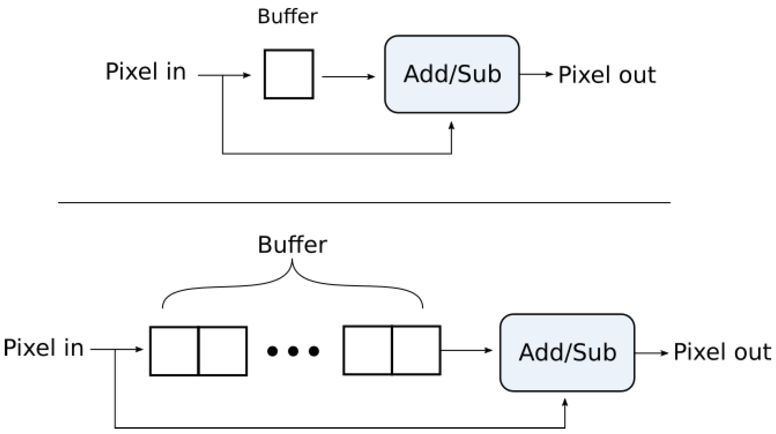
All convolutions in jet feature transforms require the addition or subtraction of two pixels. This is accomplished by feeding the pixels into a buffer, where the incoming pixel is added or subtracted from the pixel at the end of the buffer, as shown in Figure 10. Convolutions in the x direction (along the rows) require only a single pixel to be buffered due to the fact that the image sensor transmits pixels in row major order. Convolutions in the y direction, however, require pixel buffers to be the width of input image. A pixel must wait until a whole row of pixels is read in for its neighboring pixel to be fed into the system.
With units for convolution in both the x and y directions, an array of convolutional units are connected to produce every jet feature for a given multiscale local jet. Each ECO Jet Feature can consist of multiple scaling factors and partial derivatives in both the x and y directions. With these four basic types of building blocks, we construct the ECO Jet Features unit to produce every possible features with a four-dimensional array of convolution units, one dimension for each type of building block. A four-dimensional array can grow quite large as the maximum number of allowed multiples of each convolution type gets larger.
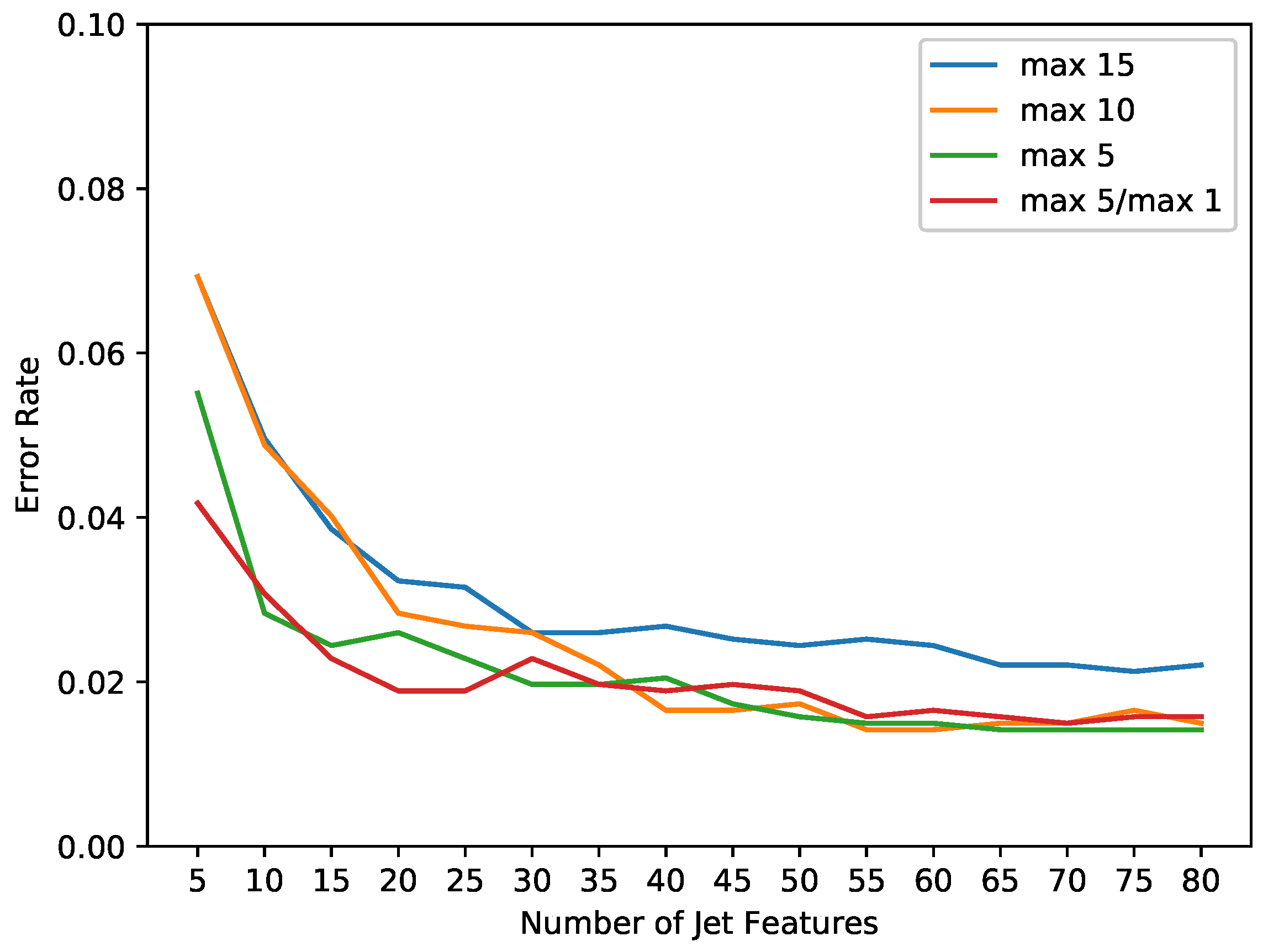
By restricting the multiscale local jet, there are fewer possible jet features. In order to see the effect of restricting the maximum allowed values for δ and σ , we tested various configurations of the BYU Fish Species dataset. This dataset is further explained in Section 6. We restricted both δ and σ to a maximum of 15, 10 and 5. Each of these configurations was trained and tested. We observed that the genetic algorithm often selected either 0 or 1 as values for δ and so a configuraction where δ 1 and σ 5 was tested as well. Figure 11 shows the average test accuracy for each of these configuration as the model is being trained. From these results we feel confident that restricting δ and σ does not hurt the algorithms accuracy significantly. It does, however, restrict the space significantly, which can mean a much more compact hardware design. In our hardware architecture we restrict δ 1 and σ 5 and only have 144 different possible jet features.
With restrictions on the maximum values for δ and σ , the size of the ECO Jet Features unit can be kept fairly small. The arrangement within the array can also help to reduce the size of the unit. Since the order of the convolutions does not matter, placing convolutional units for the y direction first, and reusing their outputs for all the other combinations requires less resources since the y direction convolutions require whole line buffers. Figure 12 shows how this array is arranged.
Computing every possible ECO Feature allows for a fully pipelined design that does not need to be reconfigured for different ECO Jet Feature models. If a new model is trained, the design does not need to be re-synthesized to use the ECO Jet Features of the new model. The newly selected features are simply routed to the classifiers instead of the old ones.

5.2. The Random Forest Unit

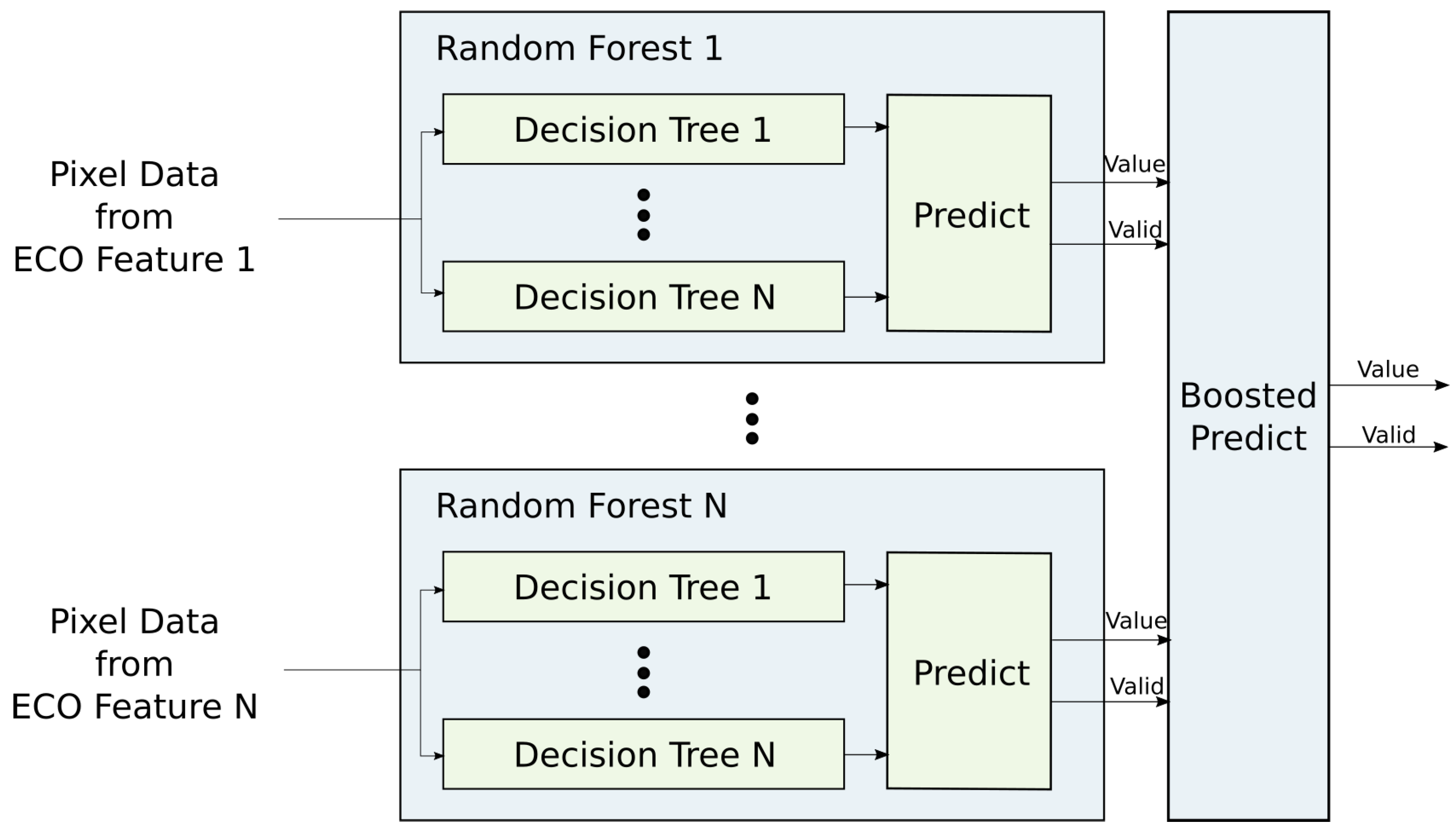
Each of the selected ECO Jet Features is connected to its own random forest. Figure 13 shows how pixel data from each ECO Jet Feature is sent to a random forest unit. Once enough pixel data is fed into a forest to make a valid prediction, a valid signal is asserted and the predicted value is sent to a prediction unit. With valid predictions from all random forest units, the prediction unit tabulates the votes and produces the a final prediction for the whole ECO Jet Features system. Votes from the random forests units are weighted inside the prediction unit according to the SAMME AdaBoost algorithm (see Section 3).
A random forest is a collection of decision trees. Figure 13 depicts individual tress inside each forest. Each tree votes individually for a particular class based on the values of specific incoming pixels. Nodes of these trees act like gates that pass their input to one of two outputs. Each node is accosted with a specific pixel location and value. If the actual value of that pixel is less than the value associated with node, the “left” output is opened. If the actual value is greater, the “right” output is opened. Each leaf node holds a prediction for the classification of the input image. Once a path is opened from the root of the tree to a leaf node, the prediction associated with that leaf is produced by the tree and a valid signal is asserted.
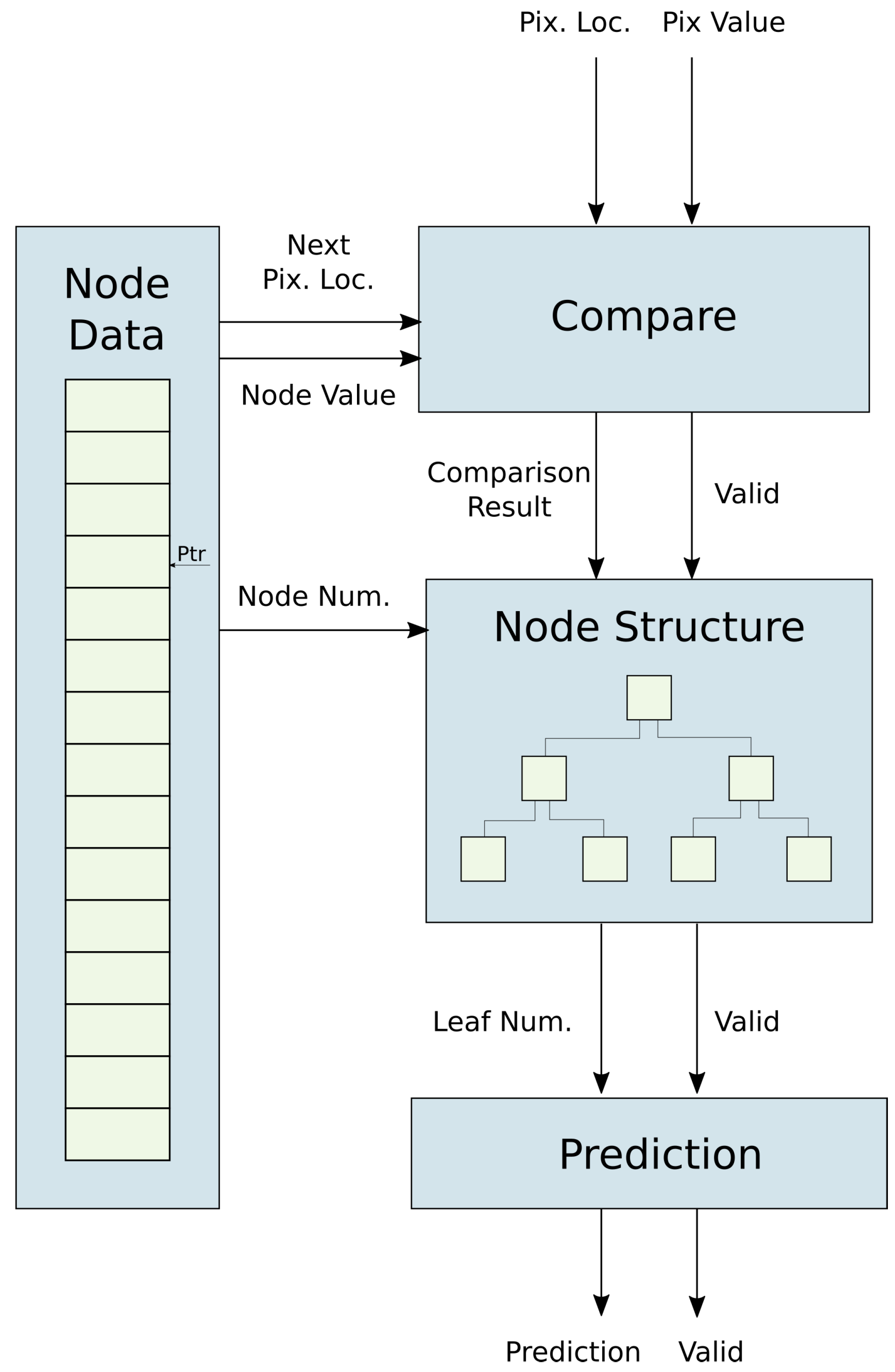
The hardware implementation for the decision tree splits the tree into four main components: node data (pixel values to compare with), pixel-node comparison unit, node structure unit and leaf prediction data, as shown in Figure 14.
The pixel value and pixel location information needed to evaluate every node in the tree is stored in the node data unit. Since pixels are streamed into the tree in row major order (left to right, top to bottom), the node data is stored in the order in which their associated pixels will arrive. The node data unit uses a pointer to note which node and pixel will arrive next. Once the pixel data arrives, the pixel-node comparison unit compares the pixel value with the value of the node. The pixel-node comparison unit then lets the tree structure know weather the pixel was greater or less than the value in the node. The tree structure unit keeps track of which nodes have been evaluated and which branches of the tree have been activated. Once a path from the root to a leaf have been activated, the prediction unit is signaled and a prediction value is sent to the output.
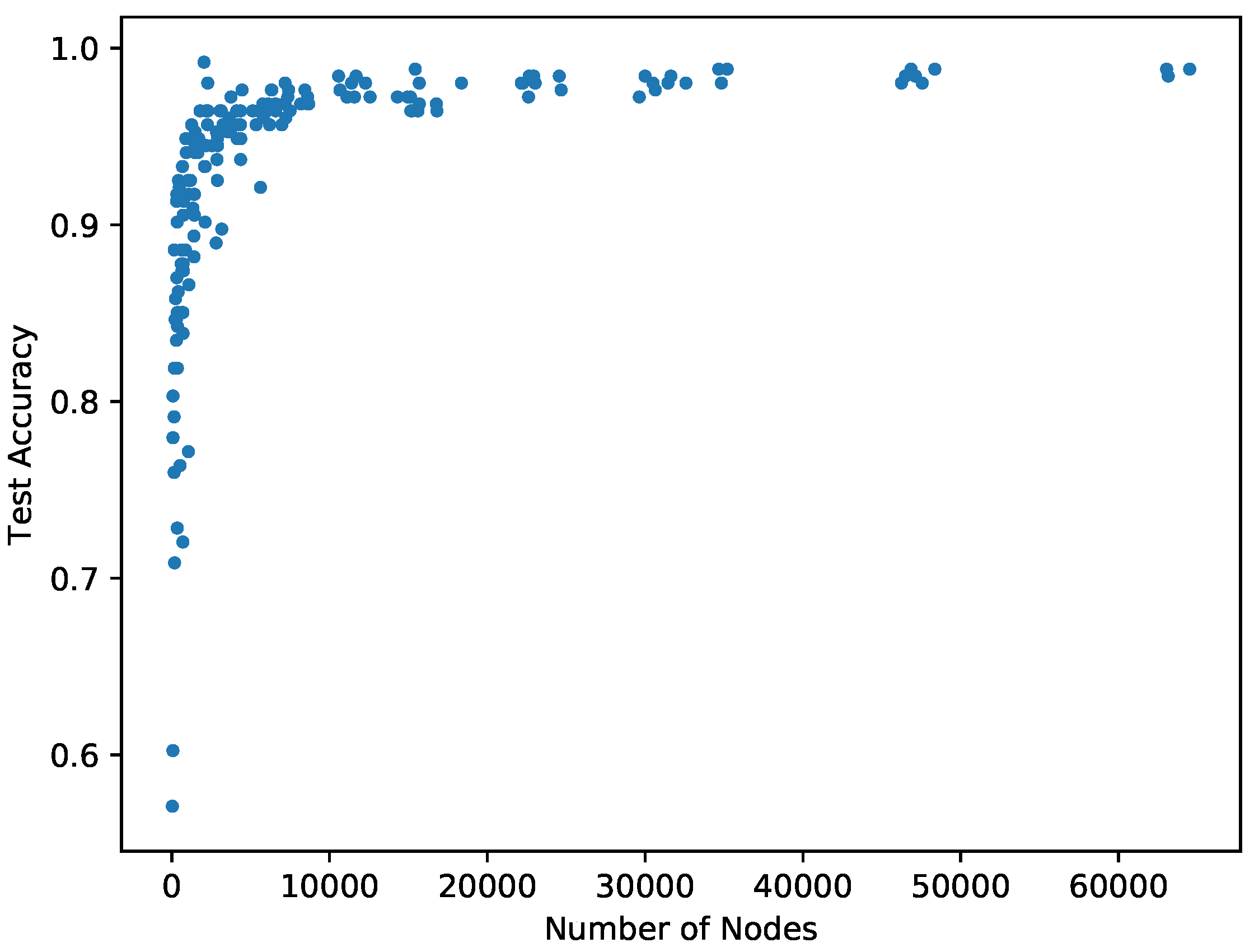
In order to select an efficient configuration, we experimented with different sizes of random forests and different numbers of jet features. We varied the number of trees in a forest, the maximum depth of each tree and total number of creatures, which corresponds with the number of forests. Figure 15 shows the accuracy of these different configurations compared with the total count of nodes in their forests. A pattern of diminished returns is apparent as models grow to be more then 3000 nodes. The models that performed best were ones with at least 10 creatures and a balance between tree count and tree depth. We used configuration of 10 features with random forests of 5 trees, each 5 levels deep. This setup requires 3150 nodes.

6. Results

6.1. Datasets

ECO Features was designed to solve visual inspection applications. These application typically involve fixed camera conditions where the objects being inspected are similar. This includes manufactured good that are being inspected for defects or agricultural produce that is being graded for size or quality. These applications usually are fairly specific and real world users do not have extremely large datasets.
We first explore the accuracy of ECO Features and ECO Jet Features on the MNIST and CIFAR-10 dataset. Both are is a common datasets used in deep learning with small images with only 10 different classes in each dataset. The MNIST dataset consists of 70,000 28 × 28 pixel images (10,000 reserved for testing) and the CIFAR-10 dataset consists of 60,000 32 × 32 pixel sized images (10,000 reserved for testing). The MNIST dataset features handwritten numerical examples and the CIFAR-10 images each consist of various objects. Examples are shown in Figure 16.
We also tested our algorithms on a dataset that is more typical for visual inspection tasks. MNIST and CIFAR-10 contain many more images than what is typically available to users solving specific visual inspection tasks. Visual inspection training sets also include less variation in object type and camera conditions than in the CIFAR-10 dataset. The MNIST and CIFAR-10 datasets consist of small images, which makes execution time atypically fast for visual inspection applications. For these reasons we also used the BYU Fish dataset in our experimentation.
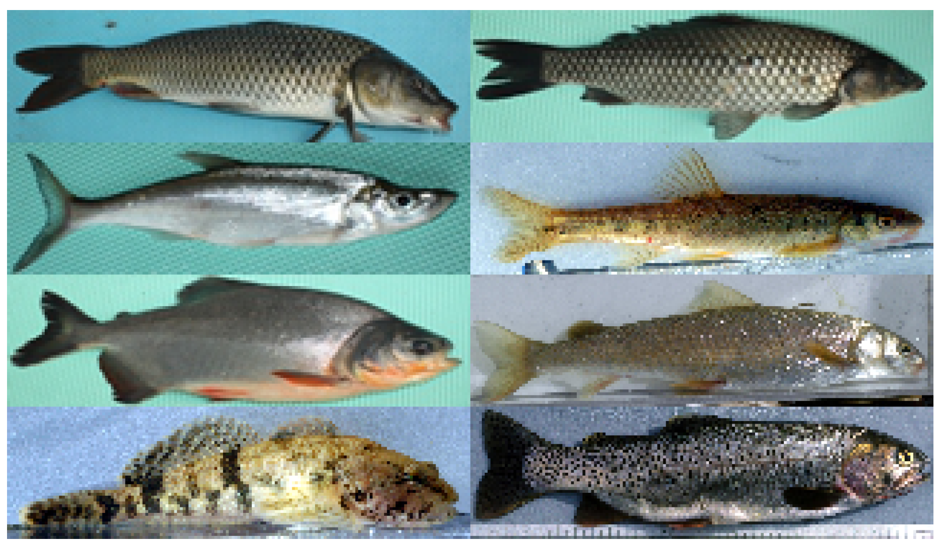
The BYU Fish dataset consists of images of fish from eight different species. The images are 161 pixels wide by 46 pixels tall. We split the dataset to include 778 training images and 254 test images. Images were converted to grayscale before being passed to the algorithm. Each specimen is oriented in the same way and the camera pose remains constant. This type of dataset is typical for visual inspection systems where camera conditions are fixed and a relatively small number of examples are available. Examples are shown in Figure 17.

6.2. Accuracy on MNIST CIFAR-10

To get a feel for how Jet Features changes the capacity of ECO Features to learn, we trained the ECO Features algorithm and the ECO Jet Features algorithm on the MNIST and CIFAR-10 datasets. These datasets have many images and were specifically designed for deep learning algorithms which can take advantage of such a large training set. We note that the absolute accuracy of these models does not compare well with the state of the art deep learning, but we use these larger datasets to fully test the capacity of our ECO Jet Features in comparison to the original ECO Features algorithm.
The images in the MNIST dataset have uniform scale and orientation. The images in the CIFAR-10 dataset are not as well conditioned. For this reason we see a higher error rate in the CIFAR-10 dataset than in the MNIST dataset. The ECO Jet Features algorithm is designed to classify images that are fairly uniform, like those in visual inspection applications where camera conditions are fixed. We include the CIFAR-10 dataset results as a means to compare the original ECO Features algorithm and the ECO Jet Features algorithm.
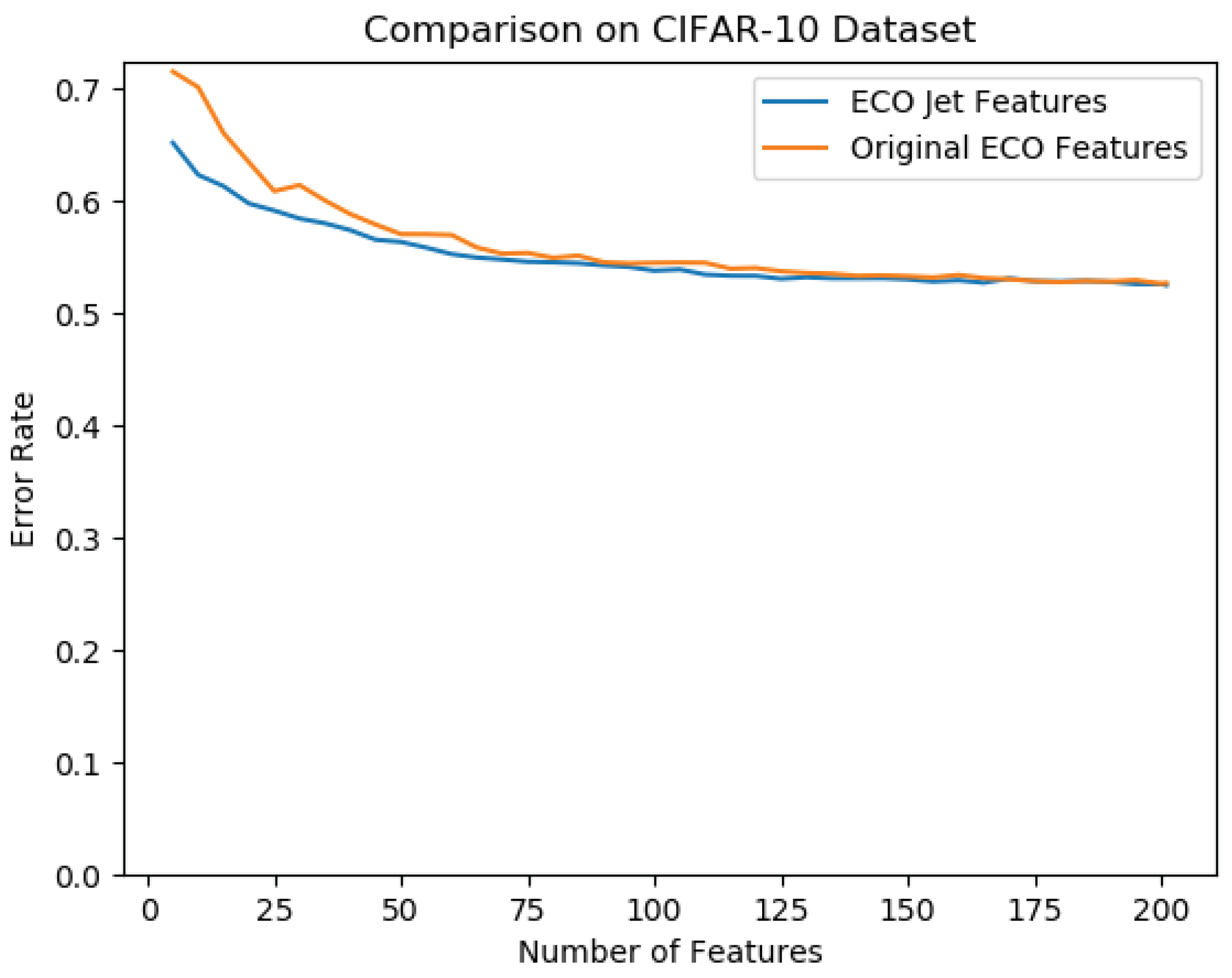
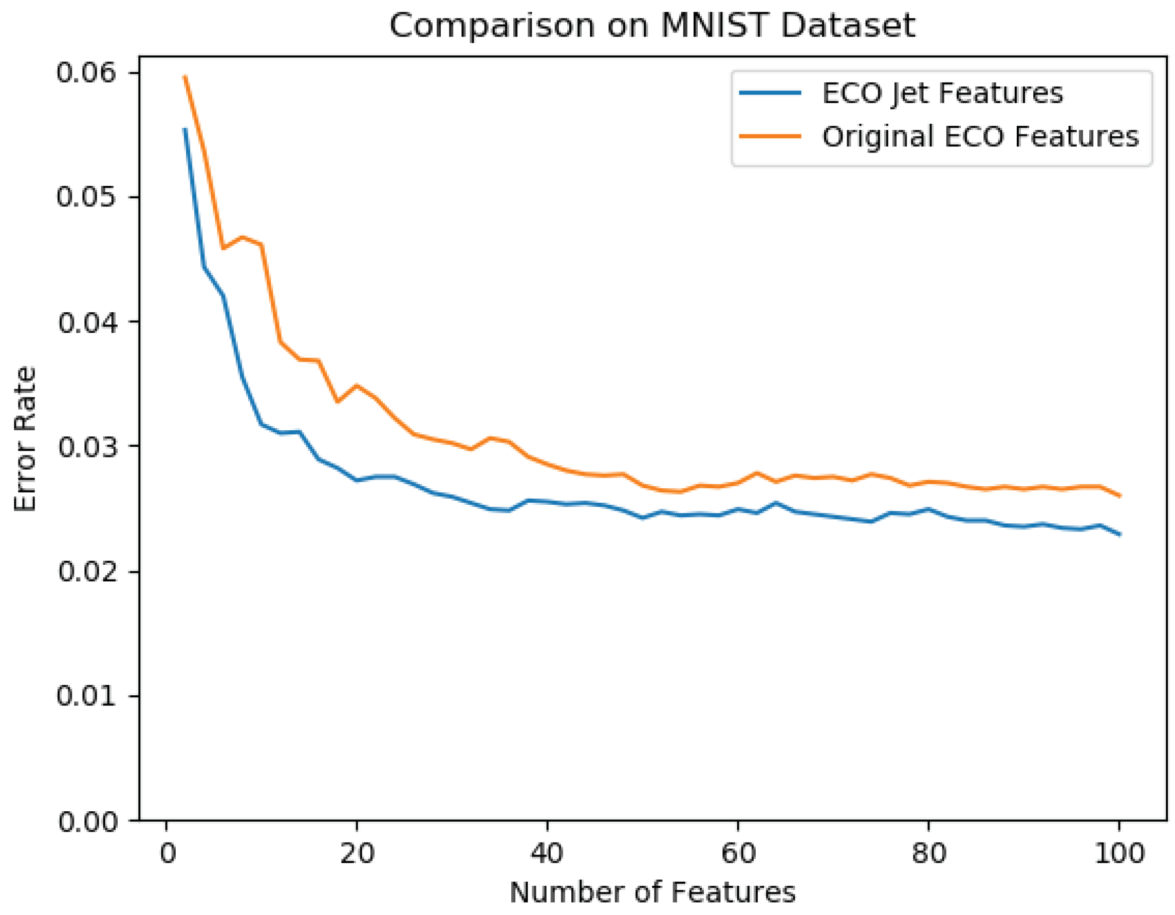
Each model was trained with random forests of 15 tress up to 15 levels deep. When testing on CIFAR-10, each model was trained 200 creatures and the accuracy as features were added is shown in Figure 18. The models were only trained to 100 creatures on MNIST where the models seem to converge, as shown in Figure 19. The CIFAR-10 results show that the models converge to similar accuracy while ECO Jet Features show a slight improvement ( 0.3%) over the original algorithm on MNIST. From these results we conclude that Jet Features introduce no noticeable loss in accuracy.

6.3. Accuracy on BYU Fish Dataset

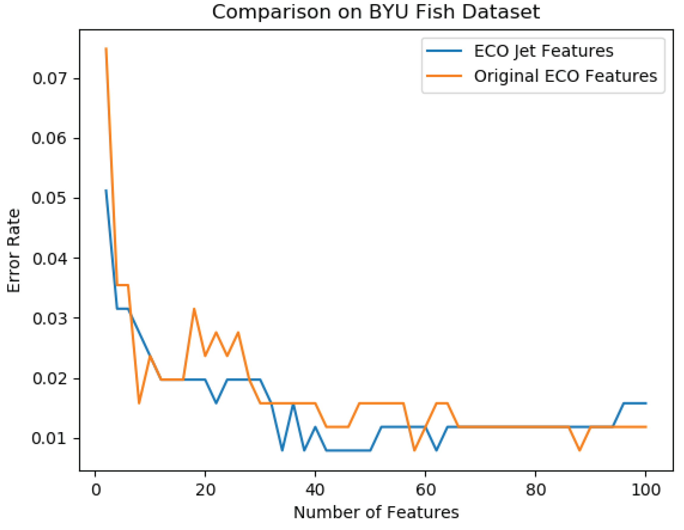
We also trained on the BYU Fish dataset with the same experamental set up that was used on the other datasets. The results are plotted in Figure 20. While the datasets do seem to converge to a similar accuracy, results from training using such a small dataset may not be quite as convincing as those obtained using larger datasets. These results were for completeness since this dataset was used in our procedure and meant for testing speed, efficiency and model size.

6.4. Software Speed Comparison

While the primary objective of the new algorithm is to be hardware friendly, it is interesting to explore the speedup gained in software. Each algorithm was implemented on a full-sized desktop PC running a Skylake i7 Intel processor, using the OpenCV library. OpenCV contains built-in functionality for most of the transforms from the original ECO Features algorithm. It also provides vectorization for Jet Feature operations.
We attempted to accelerate these algorithms using GPUs, but found this was only possible on images that were larger than 1024 × 768. Even using images that were this large did not provide much acceleration. The low computational cost of the algorithm does not justify the overhead of CPU to GPU data transfer.
A model of 30 features was created for both. The BYU Fish dataset was used because the image sizes are more typical to real world applications. The original algorithm averaged a run time of 10.95 ms and our new ECO Jet Features algorithm averaged and execution time of 2.95 ms, which is a 3.7 × speedup.

6.5. Hardware Implementation Results

Our hardware architecture was designed in SystemVerilog. It was synthesized and implemented for a Xilinx Vertex-7 FPGA using the Vivado design suite. From our analysis reported in Section 5, Figure 11 and Figure 15, we implemented a model with 10 features, 5 trees in each forest with a depth of 5, a maximum σ of 5 and maximum δ of 1. We used a round number of 100 pixels for the input image width. A model built around the BYU Fish dataset would have required only 46 pixels in its line buffers, but this length is small due to the oblong nature of fish. We feel a width 100 pixels is more representative of general visual inspection tasks.
The total utilization of available resources on the Xilinx Vertex-7 is reported in Table 2. One interesting point is that this architecture requires no Block RAM (BRAM) or Digital Signal Processing (DSPs) uints. BRAMs are dedicated RAM blocks that are built into the FPGA fabric. DSPs are generally used for more complex arithmetic operations, like general convolution. Our architecture, however, is compact enough and simple enough to not require either of these resources and instead host all of its logic in the main FPGA fabric. Look Up Tables (LUTs), make up the majority of the fabric area and are used to store all data and perform logic operations.
To give a quick reference of FPGA utilization for a CNN on a similar Vertex 7 FPGA, Prost-Boucle et al. [39] reported using 22 % to 74.4 % of the 52.6 Mb of total BRAM memory for various sizes of the model. Our model did not require the use of any of these BRAM memory units. When comparing the number of LUTs used as logic, Prost-Boucle et al. used 112 % more than our model in their smallest model and 769 % more on their larger more accurate model.
The pixel clock speed can safely reach 200 MHz. Since the design is fully pipelined around the pixel clock, images from the BYU Fish dataset could, in theory, be processed in 37 μ s. This is a 78.3× speedup over the software implementation on full sized desktop PC. A custom silicon design could be even faster than this FPGA implementation.
Table 3 shows the relative sizes for individual units of the design. Some FPGA logic slices are shared between units and the sum of the individual unit counts exceeds the totals listed in Table 2. With a setup of 10 creatures, 5 trees per forest with a depth of 5, the Jet Features Unit makes up about 70 % of the total design. However, since this unit is generating every jet in the muliscale local jet, it does not grow as more features are added to the model. We showed in Figure 11 that using a large local jet does not necessarily improve performance.
The Random Forest unit makes up less then 35 % percent of the design in all aspects other than LUT units that are used as memory, which is a subset of total LUTs. But, only 10 features were used and more could be added to increase accuracy as shown in Figure 20. Extrapolating out from these numbers, if all 144 possible features were added to this design, only 30 % of resources available to the Vertex-7 would be used and 87.9 % of them will be dedicated to the Random Forests Unit.
These results show how compact this architecture is. The simple operations and feed forward paths used in this design could very feasibly be implemented in custom silicon as well.

7. Conclusions

We have presented Jet Features, learned convolutional kernels that are efficient in both software and hardware implementations. We applied them to the ECO Features algorithm. This change to the algorithm allows faster software execution and hardware implementation. In software, the algorithm experiences a 3.7× speedup with no noticeable loss in accuracy. We also presented a compact hardware architecture for our new algorithm that is fully pipelined and parallel. On a FPGA, this architecture can process images in 37 μ s, a 78.3× speedup over the improved software implementation.
Jet Features are related to the idea of multiscale local jets. Large groups of these transforms can be calculated in parallel. They incorporate many other common image transforms such as the Gaussian blur, Sobel edge detector and Laplacian transform. The simple operators required to calculate jet features allows them to be easily implemented in hardware in a completely pipelined and parallel fashion.
With a compact classification architecture for visual inspection, automatic visual inspection logic can be embedded into image sensors and compact hardware systems. Visual inspection systems can be made smaller, cheaper and available to a wider range of visual inspection applications.

Author Contributions

Conceptualization, T.S. and D.-J.L.; Methodology, T.S.; Software, T.S.; Validation, T.S.; Formal Analysis, T.S.; Investigation, T.S.; Resources, D.-J.L.; Data Curation, T.S.; Writing—Original Draft Preparation, T.S.; Writing—Review and Editing, T.S. and D.-J.L.; Visualization, T.S.; Supervision, D.-J.L.; Project Administration, D.-J.L.; Funding Acquisition, D.-J.L.

Funding

This project was supported by the Small Business Innovation Research program of the U.S. Department of Agriculture, grant number #2015-33610-23786.

Conflicts of Interest

The authors declare no conflict of interest.

References

  1. Hubara, I.; Courbariaux, M.; Soudry, D.; El-Yaniv, R.; Bengio, Y. Binarized Neural Networks. In Advances in Neural Information Processing Systems 29; Lee, D.D., Sugiyama, M., Luxburg, U.V., Guyon, I., Garnett, R., Eds.; Curran Associates, Inc.: Dutchess County, NY, USA, 2016; pp. 4107–4115. [Google Scholar]
  2. Howard, A.G.; Zhu, M.; Chen, B.; Kalenichenko, D.; Wang, W.; Weyand, T.; Andreetto, M.; Adam, H. MobileNets: Efficient Convolutional Neural Networks for Mobile Vision Applications. arXiv 2017, arXiv:1704.04861. [Google Scholar]
  3. Lillywhite, K.; Tippetts, B.; Lee, D.J. Self-tuned Evolution-COnstructed features for general object recognition. Pattern Recognit. 2012, 45, 241–251. [Google Scholar] [CrossRef]
  4. Lillywhite, K.; Lee, D.J.; Tippetts, B.; Archibald, J. A feature construction method for general object recognition. Pattern Recognit. 2013, 46, 3300–3314. [Google Scholar] [CrossRef]
  5. Asano, S.; Maruyama, T.; Yamaguchi, Y. Performance comparison of FPGA, GPU and CPU in image processing. In Proceedings of the 2009 International Conference on Field Programmable Logic and Applications, Prague, Czech Republic, 31 August–2 September 2009; pp. 126–131. [Google Scholar] [CrossRef]
  6. Dawood, A.S.; Visser, S.J.; Williams, J.A. Reconfigurable FPGAS for real time image processing in space. In Proceedings of the 2002 14th International Conference on Digital Signal Processing, DSP 2002 (Cat. No. 02TH8628), Santorini, Greece, 1–3 July 2002; Volume 2, pp. 845–848. [Google Scholar] [CrossRef]
  7. Fahmy, S.A.; Cheung, P.Y.K.; Luk, W. Novel FPGA-based implementation of median and weighted median filters for image processing. In Proceedings of the International Conference on Field Programmable Logic and Applications, Tampere, Finland, 24–26 August 2005; pp. 142–147. [Google Scholar] [CrossRef]
  8. Birla, M.K. FPGA Based Reconfigurable Platform for Complex Image Processing. In Proceedings of the 2006 IEEE International Conference on Electro/Information Technology, East Lansing, MI, USA, 7–10 May 2006; pp. 204–209. [Google Scholar] [CrossRef]
  9. Jin, S.; Cho, J.; Pham, X.D.; Lee, K.M.; Park, S.; Kim, M.; Jeon, J.W. FPGA Design and Implementation of a Real-Time Stereo Vision System. IEEE Trans. Circuits Syst. Vid. Technol. 2010, 20, 15–26. [Google Scholar] [CrossRef]
  10. Amaricai, A.; Gavriliu, C.; Boncalo, O. An FPGA sliding window-based architecture harris corner detector. In Proceedings of the 2014 24th International Conference on Field Programmable Logic and Applications (FPL), Munich, Germany, 2–4 September 2014; pp. 1–4. [Google Scholar] [CrossRef]
  11. Qasaimeh, M.; Zambreno, J.; Jones, P.H. A Modified Sliding Window Architecture for Efficient BRAM Resource Utilization. In Proceedings of the 2017 IEEE International Parallel and Distributed Processing Symposium Workshops (IPDPSW), Orlando, FL, USA, 29 May–2 June 2017; pp. 106–114. [Google Scholar] [CrossRef]
  12. Mohammad, K.; Agaian, S. Efficient FPGA implementation of convolution. In Proceedings of the 2009 IEEE International Conference on Systems, Man and Cybernetics, San Antonio, TX, USA, 11–14 October 2009; pp. 3478–3483. [Google Scholar] [CrossRef]
  13. Chang, C.J.; Huang, Z.Y.; Li, H.Y.; Hu, K.T.; Tseng, W.C. Pipelined operation of image capturing and processing. In Proceedings of the 5th IEEE Conference on Nanotechnology, Nagoya, Japan, 11–15 July 2005; Volume 1, pp. 275–278. [Google Scholar] [CrossRef]
  14. Courbariaux, M.; Bengio, Y.; David, J.P. Training deep neural networks with low precision multiplications. arXiv 2014, arXiv:1412.7024. [Google Scholar]
  15. Sun, W.; Zeng, H.; Yang, Y.E.; Prasanna, V. Throughput-Optimized Frequency Domain CNN with Fixed-Point Quantization on FPGA. In Proceedings of the 2018 International Conference on ReConFigurable Computing and FPGAs (ReConFig), Cancun, Mexico, 3–5 December 2018; pp. 1–8. [Google Scholar] [CrossRef]
  16. Zhou, Y.; Jiang, J. An FPGA-based accelerator implementation for deep convolutional neural networks. In Proceedings of the 2015 4th International Conference on Computer Science and Network Technology (ICCSNT), Harbin, China, 19–20 December 2015; Volume 1, pp. 829–832. [Google Scholar] [CrossRef]
  17. Zhu, M.; Kuang, Q.; Lin, J.; Luo, Q.; Yang, C.; Liu, M. A Z Structure Convolutional Neural Network Implemented by FPGA in Deep Learning. In Proceedings of the IECON 2018—44th Annual Conference of the IEEE Industrial Electronics Society, Washington, DC, USA, 21–23 October 2018; pp. 2677–2682. [Google Scholar] [CrossRef]
  18. Farabet, C.; Poulet, C.; Han, J.Y.; LeCun, Y. CNP: An FPGA-based processor for Convolutional Networks. In Proceedings of the 2009 International Conference on Field Programmable Logic and Applications, Prague, Czech Republic, 31 August–2 September 2009; pp. 32–37. [Google Scholar] [CrossRef]
  19. Zhang, C.; Li, P.; Sun, G.; Guan, Y.; Xiao, B.; Cong, J. Optimizing FPGA-based Accelerator Design for Deep Convolutional Neural Networks. In Proceedings of the 2015 ACM/SIGDA International Symposium on Field-Programmable Gate Arrays (FPGA ’15), Monterey, CA, USA, 22–24 February 2015; ACM: New York, NY, USA, 2015; pp. 161–170. [Google Scholar] [CrossRef]
  20. Ding, R.; Liu, Z.; Blanton, R.D.S.; Marculescu, D. Quantized deep neural networks for energy efficient hardware-based inference. In Proceedings of the 2018 23rd Asia and South Pacific Design Automation Conference (ASP-DAC), Jeju Island, Korea, 22–25 January 2018; pp. 1–8. [Google Scholar] [CrossRef]
  21. Natsui, M.; Chiba, T.; Hanyu, T. MTJ-Based Nonvolatile Ternary Logic Gate for Quantized Convolutional Neural Networks. In Proceedings of the 2018 IEEE SOI-3D-Subthreshold Microelectronics Technology Unified Conference (S3S), Burlingame, CA, USA, 15–18 October 2018; pp. 1–2. [Google Scholar] [CrossRef]
  22. Zhou, S.; Ni, Z.; Zhou, X.; Wen, H.; Wu, Y.; Zou, Y. DoReFa-Net: Training Low Bitwidth Convolutional Neural Networks with Low Bitwidth Gradients. arXiv 2016, arXiv:1606.06160. [Google Scholar]
  23. Nakahara, H.; Fujii, T.; Sato, S. A fully connected layer elimination for a binarized convolutional neural network on an FPGA. In Proceedings of the 2017 27th International Conference on Field Programmable Logic and Applications (FPL), Gent, Belgium, 4–6 September 2017; pp. 1–4. [Google Scholar] [CrossRef]
  24. Guo, P.; Ma, H.; Chen, R.; Li, P.; Xie, S.; Wang, D. FBNA: A Fully Binarized Neural Network Accelerator. In Proceedings of the 2018 28th International Conference on Field Programmable Logic and Applications (FPL), Dublin, Ireland, 27–31 August 2018; pp. 51–513. [Google Scholar] [CrossRef]
  25. Fukuda, Y.; Kawahara, T. Stochastic weights binary neural networks on FPGA. In Proceedings of the 2018 7th International Symposium on Next Generation Electronics (ISNE), Taipei, Taiwan, 7–9 May 2018; pp. 1–3. [Google Scholar] [CrossRef]
  26. Nurvitadhi, E.; Sheffield, D.; Sim, J.; Mishra, A.; Venkatesh, G.; Marr, D. Accelerating Binarized Neural Networks: Comparison of FPGA, CPU, GPU, and ASIC. In Proceedings of the 2016 International Conference on Field-Programmable Technology (FPT), Xi’an, China, 7–9 December 2016; pp. 77–84. [Google Scholar] [CrossRef]
  27. Yonekawa, H.; Nakahara, H. On-Chip Memory Based Binarized Convolutional Deep Neural Network Applying Batch Normalization Free Technique on an FPGA. In Proceedings of the 2017 IEEE International Parallel and Distributed Processing Symposium Workshops (IPDPSW), Orlando, FL, USA, 29 May–2 June 2017; pp. 98–105. [Google Scholar] [CrossRef]
  28. Umuroglu, Y.; Fraser, N.J.; Gambardella, G.; Blott, M.; Leong, P.; Jahre, M.; Vissers, K. FINN. In Proceedings of the 2017 ACM/SIGDA International Symposium on Field-Programmable Gate Arrays—FPGA ’17, Monterey, CA, USA, 22–24 February 2017; ACM Press: New York, NY, USA, 2017; pp. 65–74. [Google Scholar] [CrossRef] [Green Version]
  29. Blott, M.; Preußer, T.B.; Fraser, N.J.; Gambardella, G.; O’brien, K.; Umuroglu, Y.; Leeser, M.; Vissers, K. FINN-R: An End-to-End Deep-Learning Framework for Fast Exploration of Quantized Neural Networks. ACM Trans. Reconfig. Technol. Syst. 2018, 11, 1–23. [Google Scholar] [CrossRef]
  30. Florack, L.; Ter Haar Romeny, B.; Viergever, M.; Koenderink, J. The Gaussian Scale-space Paradigm and the Multiscale Local Jet. Int. J. Comput. Vis. 1996, 18, 61–75. [Google Scholar] [CrossRef]
  31. Lillholm, M.; Pedersen, K.S. Jet based feature classification. In Proceedings of the 17th International Conference on Pattern Recognition (ICPR 2004), Cambridge, UK, 23–26 August 2004; Volume 2, pp. 787–790. [Google Scholar]
  32. Larsen, A.B.L.; Darkner, S.; Dahl, A.L.; Pedersen, K.S. Jet-Based Local Image Descriptors. In Proceedings of the 12th European Conference on Computer Vision, Florence, Italy, 7–13 October 2012; Fitzgibbon, A., Lazebnik, S., Perona, P., Sato, Y., Schmid, C., Eds.; Springer: Berlin/Heidelberg, Germany, 2012; pp. 638–650. [Google Scholar] [Green Version]
  33. Manzanera, A. Local Jet Feature Space Framework for Image Processing and Representation. In Proceedings of the 2011 Seventh International Conference on Signal Image Technology Internet-Based Systems, Dijon, France, 28 November–1 December 2011; pp. 261–268. [Google Scholar] [CrossRef]
  34. Krizhevsky, A.; Sutskever, I.; Hinton, G.E. ImageNet Classification with Deep Convolutional Neural Networks. In Proceedings of the 25th International Conference on Neural Information Processing Systems (NIPS’12); Curran Associates Inc.: Dutchess County, NY, USA, 2012; Volume 1, pp. 1097–1105. [Google Scholar]
  35. Breiman, L. Random Forests. Mach. Learn. 2001, 45, 5–32. [Google Scholar] [CrossRef] [Green Version]
  36. Zhu, J.; Rosset, S.; Zou, H.; Hastie, T. Multi-class AdaBoost. Stat. Interface 2009, 2, 349–360. [Google Scholar] [CrossRef] [Green Version]
  37. Freund, Y.; Schapire, R.E. A Decision-Theoretic Generalization of On-Line Learning and an Application to Boosting. J. Comput. Syst. Sci. 1997, 55, 119–139. [Google Scholar] [CrossRef] [Green Version]
  38. Zhang, M.; Lee, D.J.; Lillywhite, K.; Tippetts, B. Automatic quality and moisture evaluations using Evolution Constructed Features. Comput. Electron. Agric. 2017, 135, 321–327. [Google Scholar] [CrossRef] [Green Version]
  39. Prost-Boucle, A.; Bourge, A.; Pétrot, F.; Alemdar, H.; Caldwell, N.; Leroy, V. Scalable high-performance architecture for convolutional ternary neural networks on FPGA. In Proceedings of the 2017 27th International Conference on Field Programmable Logic and Applications (FPL), Ghent, Belgium, 4–8 September 2017; pp. 1–7. [Google Scholar] [CrossRef]
Figure 1. An example a separable filter. A 3 × 3 Gaussian kernel can be separated into two convolutions with smaller kernels.
Electronics 08 00588 g001
Figure 2. The four basic kernels of all Jet Features. The top two kernels can be thought of as scaling or blurring factors. The bottom two perform derivatives in the either the x or y direction. Every Jet Feature is simply a series of convolutions with any number of each of these kernels. The order does not matter.
Electronics 08 00588 g002
Figure 3. These examples demonstrate how the Gaussian kernel and Sobel kernels are examples of Jet Features. These 3 × 3 kernels can be broken down into a series of four convolutions with the two cell Jet Feature kernels. The Sobel kernels are similar to the Gaussian, but one of the scaling factors is replaced with a partial derivative.
Electronics 08 00588 g003
Figure 4. An example of a hypothetical ECO Feature made up of three transforms. The top boxes represent the type of each transform. The boxes below show each transform’s associated parameters. The number of transforms, transform types and parameters of each transforms are randomly initialized and then evolved through a genetic algorithm.
Electronics 08 00588 g004
Figure 5. An example of mutation (top) and crossover (bottom). Mutation will only change the parameters of a given ECO Feature. Crossover takes the first part of one feature and appends the latter part of another feature to it.
Electronics 08 00588 g005
Figure 6. A example paring of an ECO Feature with a random forest classifier. Every ECO Feature is paired with its own classifier. Originally, perceptrons were used, but in our work, random forests are used which offer multiclass classification.
Electronics 08 00588 g006
Figure 7. A system diagram of the original ECO Features Algorithm. Each classifier has its own ECO Feature transform. The outputs of each classifier are collected into a weighted summation to determine the final prediction.
Electronics 08 00588 g007
Figure 8. How mutation (top) and crossover (bottom) are defined for Jet Features.
Electronics 08 00588 g008
Figure 9. System diagram for the ECO Jet architecture. The Jet Features Unit computes every feature for a given multiscale local jet on an input image. A router connects only the ones that were selected during training to a corresponding random forest. The forests each vote on a final prediction.
Electronics 08 00588 g009
Figure 10. Convolution units. The top unit shows only a single buffer needed for convolution along rows in the x direction. The bottom unit shows a large buffer used for convolution along the columns in the y direction.
Electronics 08 00588 g010
Figure 11. Comparison of multiscale local jets. The maximum allowable variance in Gaussian blur and order of differentiation was limited by 15, 10 and 5. A fourth case was tested where variance in Gaussian blur was bounded by 5 and order of differentiation and was bounded by 1.
Electronics 08 00588 g011
Figure 12. The array of convolutions in the ECO Jet Features unit. The first dimension consists of five scaling factor units ( σ 5 ) that use addition convolutions as shown in Figure 10. The second dimension consists of a single partial derivative factor for each of the outputs of the previous dimension and the input ( δ 1 ). The angled blocks represent further convolutions, suggesting the third and forth dimensions.
Electronics 08 00588 g012
Figure 13. The arrangement of forests and trees for ECO Jet Feature predictions. Each ECO Jet Feature drives in input of a random forest. Each random forest is made up of multiple decision trees. Predictions of tree are tabulated to make the decision of a single forest. The votes from forests are weighted and tabulated to form the prediction for the entire system.
Electronics 08 00588 g013
Figure 14. The hardware structure of a decision tree. The node data unit holds the pixel value and pixel location information for the pixel each nodes is compared to. It outputs the data for the next pixel that will be streamed in. The node-pixel comparison unit waits for a match from the incoming pixel location from the input and the next pixel location from the node data unit. The pixel and node values are compared. The result is sent to the node structure unit. Once a leaf is activated in the tree structure, the prediction unit is signaled and a prediction is issued from the tree.
Electronics 08 00588 g014
Figure 15. Comparison of test accuracy to the number of total nodes the random forests. Various number of trees, forests and depths of trees were tested.
Electronics 08 00588 g015
Figure 16. Examples from the MNIST dataset (top) with handwritten digits. Examples from the CIFAR-10 dataset (bottom). Classes include airplane, bird, car, cat, deer, dog, frog, horse, ship and truck.
Electronics 08 00588 g016
Figure 17. Examples from the BYU Fish dataset. Each image is of a different fish species.
Electronics 08 00588 g017
Figure 18. Accuracy comparison between the original ECO Features algorithm and the ECO Jet Features algorithm on CIFAR-10. Once the models seem to converge, there is no evidence of lost accuracy in the ECO Jet Features model.
Electronics 08 00588 g018
Figure 19. Accuracy comparison between the original ECO Features algorithm and the ECO Jet Features algorithm on MNIST. Once the models seem to converge, ECO Jet Features seem to have a slight edge in accuracy, about 0.3%.
Electronics 08 00588 g019
Figure 20. Accuracy comparison between the original ECO Features algorithm and the ECO Jet Features algorithm on the BYU Fish dataset.
Electronics 08 00588 g020
Table 1. The pool of possible image transforms used in the ECO Features Algorithm.
TransformParametersTransformParameters
Gabor filter6Sobel operator4
Gradient1Difference of Gaussians2
Square root0Morphological erode1
Gaussian blur1Adaptive thresholding3
Histogram1Hough lines2
Hough circles2Fourier transform1
Normalize3Histogram equalization0
Log0Laplacian Edge1
Median blur1Distance transform2
Integral image1Morphological dilate1
Canny edge4Harris corner strength3
Rank transform0Census transform0
Resize1Pixel statistics2
Table 2. ECO Jet Features architecture total hardware usage on a Kintex-7 325 FPGA using 10 creatures, 5 trees at a depth of 5.
ResourceNumber UsedPercent of Available
Total Slices10,8684.9%
Total LUTs34,5524.9%
LUTs as Logic31,6444.4%
LUTs as Memory29081.0%
Flip Flops17,1321.2%
BRAMs00%
DSPs00%
Table 3. The hardware usage for individual design units.
UnitSlicesTotal LUTsLUTs as LogicLUTs as MemoryFlip Flops
Jet Features Unit759323,25322,37787611,411
Random Forests Unit374111,080908020005080
Individual Random Forests3741108908200508
Individual Decision Trees732101714093
Feature router4940400520
AdaBoost Tabulation6118014832121