Article

Dynamic Network Topology Control of Branch-Trimming Robot for Transmission Lines

1
School of Power and Mechanical Engineering, Wuhan University, Wuhan 430072, China
2
School of Mechanical Engineering and Automation, Wuhan Textile University, Wuhan 430073, China
3
State Grid Jilin Electric Power Co., Ltd., Baishan Power Company, Baishan 134300, China
*
Authors to whom correspondence should be addressed.
Electronics 2019, 8(5), 549; https://doi.org/10.3390/electronics8050549
Submission received: 13 March 2019 / Revised: 2 May 2019 / Accepted: 9 May 2019 / Published: 15 May 2019

Abstract

:
With the development of engineering technology, the distributed design-based Branch-Trimming Robot (BTR) has been used to ensure the power supply security of transmission lines. However, it remains difficult to combine distributed BTRs with a wireless sensor network to build an efficient multi-robot system. To achieve this combination, a dynamic network topology control method was proposed, combining the motion characteristics of robots with the structure of a distributed wireless sensor network. In addition, a topology-updating mechanism based on node signal strength was adopted as well. To achieve efficient data transmission for distributed multi-robot systems, the present study focused on the design of a distributed network model and a dynamic network topology control strategy. Several simulation and test scenarios were implemented, and the changes of network performance under different parameters were studied. Furthermore, the real scene-based dynamic topology control method considers the relationship between network performance and antenna layout.

1. Introduction

A normal power supply is one of people’s basic needs. Overhead transmission lines are often affected by trees, especially when their branches enter the safety area of energized transmission lines, the risk of blackouts and bush firing will increase [1]. Power utilities, despite the significant expenditure in tree trimming, trim trees to minimize the tree-caused power outages [2]. Due to the possibility of contact with the energized power lines, work at height, and the tools used, there is a huge risk when trimming around overhead power lines. Robotic systems, especially distributed multi-robot systems, can help significantly increase productivity and create a safe environment to perform tasks.
In recent decades, multi-robot, distributed robot, and distributed network systems have become hot topics [3,4]. Multi-robot systems controlled in distributed intelligent network systems have been used for surveillance, exploration, and transmission line monitoring [5,6]. To address the problems related to power supply security caused by the rapid growth of vegetation around transmission lines, a multi-robot system called the Branch-Trimming Robot (BTR) was developed. To adapt to the complex and changeable vegetation coverage around transmission lines, the distributed control system was adopted in the BTR, thereby expanding the mobile space and widening the operational scope of the robot.
Transmission lines are used to transmit electric energy along large distances, which usually traverse virgin forest and unmanned areas [7]. The BTR was designed to address power supply security problems related to the rapid growth of vegetation by trimming around transmission lines. Due to the special environments and insulation requirements around energized transmission lines, wireless communication was adopted in the BTR. However, the use of public networks such as 4G and 5G is limited in virgin forest and unmanned area [6]. Additionally, a spatially discrete multi-robot system also makes it difficult to achieve robot information interaction and cooperative control. In summary, there are still challenges to achieve intelligent monitoring and improve the efficiency of the BTR.
Wireless sensor networks (WSNs) constitute a practical remote monitoring technique that has received extensive attention. WSNs are beneficial for analyzing and optimizing the network performance of the BTR, and provide a theoretical basis and development for researching the BTR and other distributed control systems. Topology is a major concern of WSNs, since it has a close relation to network performance, e.g., packet delivery ratio, end-to-end delay, etc. However, since the components of the BTR exhibit spatial dispersion and mobility, a fixed topology may no longer satisfy the network performance requirements of the BTR. Accordingly, it is vital to research intelligent topology control for the BTR.
A multi-robot system named the BTR was developed to achieve the detection and trimming of tree branches around energized transmission lines based on reference [8]. The BTR controlled in a distributed network system works in a single span to trim hazard tree branches. This robot transits the acquired videos and images to a Base Station (BS) on the ground. According to the data sent from the multi-robot system, the BS instructs the multi-robot system to trim the hazard tree branches. The communication between the BTR and BS is achieved via Wi-Fi (IEEE 802.11 n) based on directional antennas installed in each component of the multi-robot system and BS. The BTR program was tested in Jilin Province of China, and the project is shown in Figure 1. However, some communication errors between the BTR and BS occurred when the BTR operated in a span between two towers. The use of a fixed topology of the multi-robot network system led to the low communication capabilities between the multi-robot system and BS.
The packet delivery ratio and end-to-end delay are two crucial indices when manipulating the BTR to detect and trim tree branches. However, the mobility of the components of the BTR and the use of directional antennas makes it difficult to confirm a suitable network topology to ensure the mentioned indices.
To solve the problems in the BTR’s detection and trimming of tree branches for transmission lines, the Distributed Branch-Trimming Robot Network (DBTRN) and Dynamic Network Topology Control Strategy (DNTCS) are proposed in this study. The DBTRN is a model to analyze the BTR, which consists of a network deployment model, mobility model, Received Signal Strength (RSS) mathematical model, and discrete time mathematical model. The network deployment model ensures that the multi-robot system is capable of detecting and trimming hazard tree branches; the mobility model classifies the process through which the BTR approaches hazard tree branches into simple motions; the RSS mathematical model predicts the RSS of each component of the BTR by combining the mobility model of the BTR and characteristics of directional antennas; lastly, the discrete time mathematical model selects the optimal path from a mobile node to the BS. Besides, the DNTCS confirms the topology of the DBTRN to improve the network performance and reliability of the DBTRN before the BTR performs a certain motion. The DNTCS ensures that the DBTRN exhibits the best network performance when the BTR approaches target hazard branches. This is achieved by the process through which each mobile node finds an optimal path to the BS, and the set of the optimal paths form the network topology of the DBTRN. The DNTCS calculates the weight of each wireless link by combining the mobility model, RSS mathematical model, and discrete time mathematical model. By comparing the values of the available weight, the optimal path from each node to the BS is selected.
In brief, a distributed network model, DBTRN, was introduced in the BTR, and a dynamic network topology control method, DNTCS—based on a discrete-time mathematic model of distributed network nodes—was proposed to improve the wireless network performance of distributed multi-robot systems. The major contributions of this study are as follows:
  • The DBTRN was developed to interpret the communication between the BS and components of the multi-robot system; components of the BTR and the BS correspond through communication nodes in the DBTRN. The DBTRN was designed to help the BTR effectively detect and trim hazard tree branches. It can also be referenced for developing other distributed multi-robot system network models.
  • Combined with the mobility model and RSS mathematical model of each node in the DBTRN, a mathematic model in accordance with graph theory was presented to interpret the interactive relationship between nodes in the multi-robot systems.
  • A novel network topology control method for multi-robot systems was introduced based on the weight calculation of each wireless link to improve the packet delivery ratio and reduce end-to-end delay. The DNTCS refers to a pre-action before the BTR performs a certain motion.
The rest of this study is organized as follows. Important relevant studies about the topology control of WSNs are presented in Section 2. The method and algorithm are shown in Section 3. The simulation and experiment results are proposed in Section 4. The results are discussed and analyzed in Section 5. Finally, conclusions are drawn in Section 6.

2. Related Work

A distributed control system and its wireless sensor network topology control technology have been extensively developed. Many multi-robot systems have been proposed to solve a broader set of complex cooperative tasks [5]. The multi-robot system has employed Unmanned Ground Vehicles (UGVs) to achieve the treasure hunt [9] and exploration [10]. Combining multi-robot systems with WSNs can improve the real-time performance of multi-robot systems.
The topology of WSNs is the set of communication links between pairs of nodes used by a routing mechanism; networks that do not employ topology control may increase packet end-to-end delay, decrease the packet delivery ratio, and reduce the robustness to nodes failures [11]. Thus, topology is vital for WSNs to ensure Quality of Service (QoS), minimize latency, and prolong the network lifetime.
Various types of topologies in WSNs (e.g., flat topology, cluster-based topology, tree-based topology, and chain-based topology) were presented in [12]. A flat-based topology is unstructured, which can cause unreliability and high end-to-end delay. A cluster-based topology is especially useful for WSNs in the case of high scalability, which can be identified by cluster selecting, cluster formation set up, and data transmission. However, the connectedness of the network may not be ensured. Chain-based topology is deployed by the selection of a header of a chain, and all the sensor nodes communicate along the chain. In this type of topology, the network lifetime is prolonged, whereas the network delay is high. When the WSN is deployed by tree-based topology, leaf nodes and root nodes will be selected, and data will flow from leaf nodes to root nodes.
The topology of WSNs can vary due to the mobility of sensor nodes. A mobility prediction model for the topology control of Mobile Ad hoc Network (MANET) based on a neural network was proposed in [13]. By forecasting the locations of mobile nodes, optimal topology was achieved by minimizing interference and reducing transmission powers. A topology control algorithm acting as a trade-off between a delay-constrained environment and minimum interference was proposed in [14], and a node is capable of adjusting transmission power if the estimated delay reaches a threshold. A method that adaptively adjusts the node transmit powers in response to topological changes and attempts to maintain a connected topology using minimum power was presented in [11,15].
Besides, topology control is usually used to offer a stable communication system for Unmanned Aerial Vehicles (UAVs). Communication structures of networks for networking UAVs were discussed in [16,17]. One of the first flight experiments with Flying Ad-Hoc Networks (FANET) architecture was performed by Stanford Research Institute (SRI) International [18]. In this study, Topology Broadcast was based on Reverse-Path Forwarding (TBRPF) [19]. A topology control protocol inspired by the potential field approach was proposed in [20], and the strength of the interconnections of UAVs was calculated, depending on both Received Signal Strength Value Indicators (RSSI) and distances between UAVs, RSSI values, and Global Positioning System (GPS) information, which was used in the topology control strategy. In [21], Proximity-Sensitivity Routing (PSR) was developed to manage the topology of the proposed network. PSR provided the selection of possible optimized routes between the ground station and the aerial nodes.
Most proposed algorithms hypothesized that isotopic antennas were used in sensor nodes, whereas mobile sensor nodes are frequently outfitted with directional antennas in practice. To address such problems, in [22], a distributed topology control mechanism for networks with directional antennas that adjusts antenna orientation in addition to transmission power was proposed, which used information about the sector of arrival instead of angle of arrival. Moreover, an optimization framework for topology control in wireless networks was introduced, and a practical and efficient distributed protocol using sectorized antennas was developed based on the RSS and interference of each node [23]. Accordingly, topology control was achieved by minimizing a function regarding the received signal strength of a communication node. Furthermore, graph connectivity is a commonly used theoretical basis in the topology control of a network system consisting of mobile robots [24,25].
An extensive application of a WSN topology control, multi-robot system inspired us to design a topology control method to improve the efficiency of BTR. In this study, our algorithm uses ideas from some of the strategies presented in this section. It can be considered a topology control strategy of a network system made up of mobile robots to maximize the data delivery ratio and minimize network delay. This strategy is based on a mobility model of mobile nodes [13,25]; link availability is achieved by estimating the RSS when using directional antennas [23], and graph theory is used to describe the network model [26,27]. More details will be given in the next section.

3. Models and Method

This section introduces a new type of Distributed Branch-Trimming Robot Network (DBTRN) model and proposes a new Dynamic Network Topology Control Strategy (DNTCS). To make this network model work efficiently, this study introduces the BTR, analyzes the movement of each part of the BTR when the BTR walks along the ground wire or works in the area below the transmission lines. In addition, the mathematic model of the DBTRN is proposed in accordance with graph theory and features of the DBTRN model. To make the calculation more accurate, the mathematical model of the RSS of each wireless node is proposed based on the characteristics of directional antennas and the mobility of each node. Finally, the DNTCS is proposed for application of the BTR.

3.1. Preliminary

Over the past decades, many types of devices have been employed to trim trees around overhead transmission lines. Vehicles, Unmanned Aerial Vehicles (UAVs), and helicopters have been used to carry apparatuses to trim branches, which may negatively affect energized transmission lines. Numerous studies have discussed the applications of branch trimming for transmission lines [1,2,28,29]. They can be separated as ground-based robots and airborne robots supported by helicopters or UAVs. However, these applications have many drawbacks:
  • Ground-based robots cannot reach remote areas (e.g., ravines and mountains).
  • The development of airborne robots is limited by high costs, low battery life, and stability.
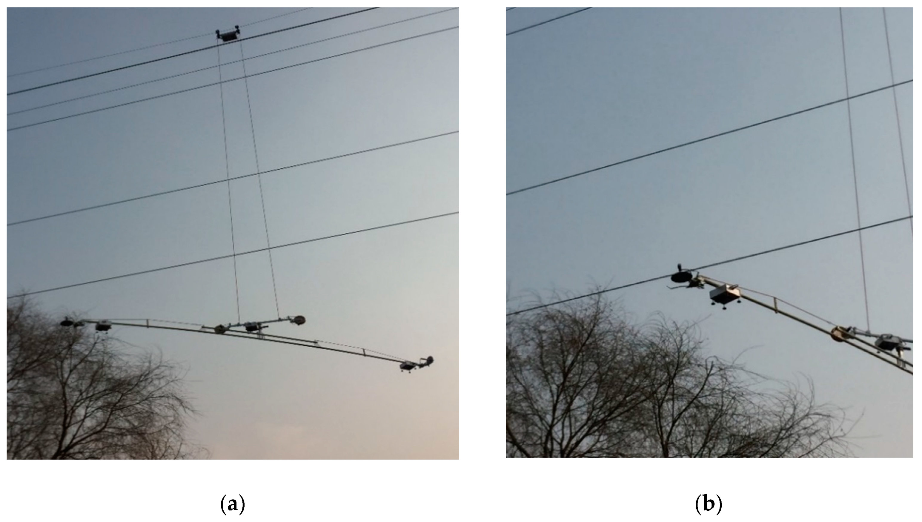
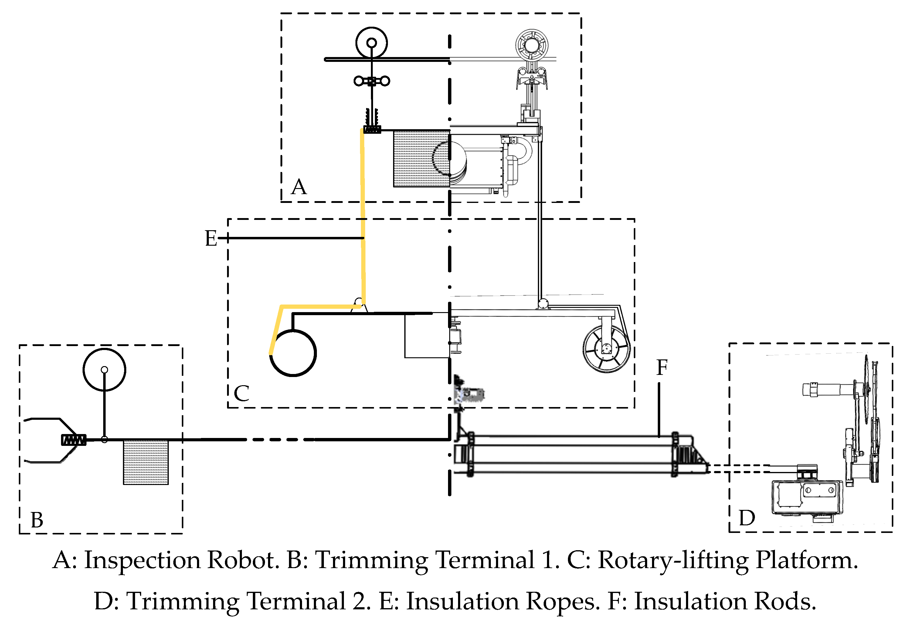
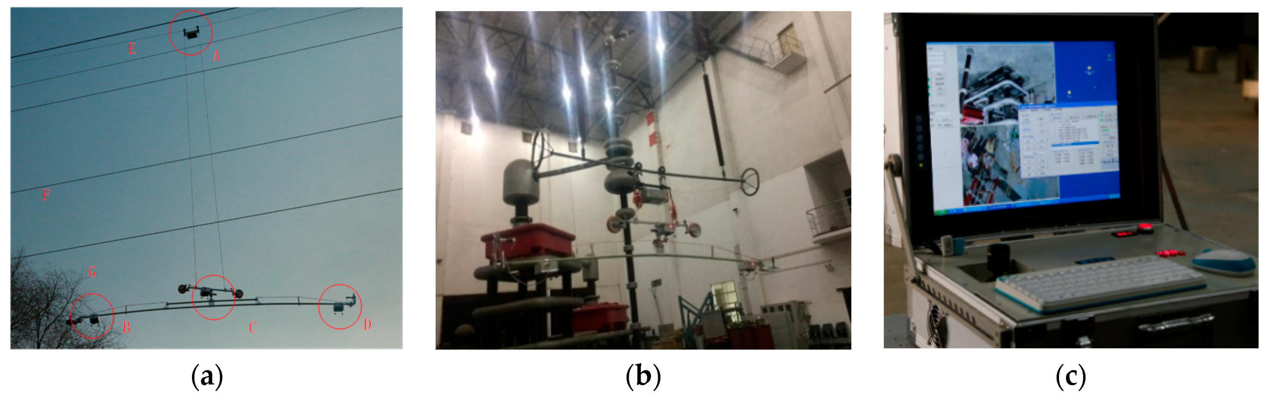
In this section, a BTR for trimming the trees around transmission lines is introduced. An abbreviated drawing of the BTR is given in Figure 2. The BTR consists of four components, including an Inspection Robot (IR), a rotary-lifting platform, and two trimming terminals. The role of the IR in the BTR is the same as that of the vehicle in a ground-based robot and that of the helicopter in an airborne robot. The IR carries the rotary-lifting platform and two trimming terminals (together known as executing mechanisms). The IR collaborates with executing mechanisms to detect and trim hazard tree branches, and the IR moves along the ground wire as a carrier of BTR. Its combined mechanism, non-collision overcoming mechanism, and inspection method were presented in [7,30]. Additionally, the IR is capable of detecting hazard branches using two Pan–Tilt–Zoom (PTZ) cameras [31].
The capabilities of the rotary-lifting platform allow the two trimming terminals to rotate around a fixed point and move in the vertical direction. The two trimming terminals were designed to detect and trim the hazard branches, and cameras also enable the detection of hazard branches. As the BTR detects and trims the hazard branches between two power towers, the IR moves along the ground wire, while the executing mechanisms work without penetrating the safety area of the energized transmission lines. Besides, it is vital to isolate the BTR from the high-voltage energized lines. Since the BTR was designed to trim branches around energized lines, insulating materials must be used in the BTR to prevent accidents (e.g., blackouts and apparatus damage) [32]. Accordingly, insulation ropes and insulation rods are introduced in the BTR; insulation ropes are used to connect the IR and executing mechanism, and insulation rods are used to connect the rotary-lifting platform and two trimming terminals. Thus, the BTR can be considered a set of sub-robots that disperse spatially in an area around transmission lines.
The detection of hazard branches is achieved by cameras installed on the IR and two trimming terminals, and the trimming of branches is performed by trimming terminals. Therefore, the reasons why the BTR can be considered a multi-robot system are as follows.
  • Each component of the BTR is an independent robot that performs a certain task in the group. Moreover, the components of BTR are outfitted with sophisticated sensors and actuators to collect information around the transmission lines and perform different types of motions, respectively.
  • The branch-trimming task is overly complex for a single robot. The trimming task is inherently distributed, and it can be separated into a set of tasks, which can be performed by the components of the BTR.
  • Branching trimming tasks can be implemented intelligently and easily based on the cooperation between the sub-robots of the BTR.
However, how the sub-robots of the BTR interact with each other is hard to explain. Among the sub-robots of the multi-robot system, the IR walks along the ground wire, and the executing mechanisms operate under the phase lines. Energized high-voltage transmission lines are parallelly distributed between the IR and the other sub-robots of the multi-robot system. Due to the voltage and current of the running transmission lines, a strong electromagnetic field and an electric field would be produced in its nearby environment. Wired communication is limited in the multi-robot system for the following reasons.
  • The phase lines that traverse the IR and the other sub-robots of the multi-robot system significantly limit the system’s use of wired communication. When the cable approaches the energized transmission line, the electromagnetic field generated by the energized transmission lines would interfere with the data running on the cable [33,34,35]. Otherwise, according to the standards for overhead transmission lines in China, no conductors will be allowed into the safety area of high-voltage energized transmission lines.
  • Using wired communication may increase the difficulty of cable management. Distances between the IR and other sub-robots vary due to the mobility of each sub-robot. Although the distances between the rotary-lifting platform and trimming terminal are fixed, the rotation of the Rotary-Lifting Platform (RP) may cause the cables to wind.
Accordingly, the capabilities of the sub-robots of the multi-robot system are limited; trimming branches around transmission lines requires the cooperation of each sub-robot. Additionally, wireless communication is used in the multi-robot system, which leads to a high packet loss rate and network delay if the network topology is not suitable. Packet loss and network delay cause errors in information collecting and motion controlling, which may decrease the efficiency of the BTR when detecting and trimming hazard tree branches. Therefore, a dynamic network topology control method is proposed to solve the network optimization problem of the BTR, which is based on a distributed network model.

3.2. Distributed Branch Trimming Robot Networks (DBTRN) Model

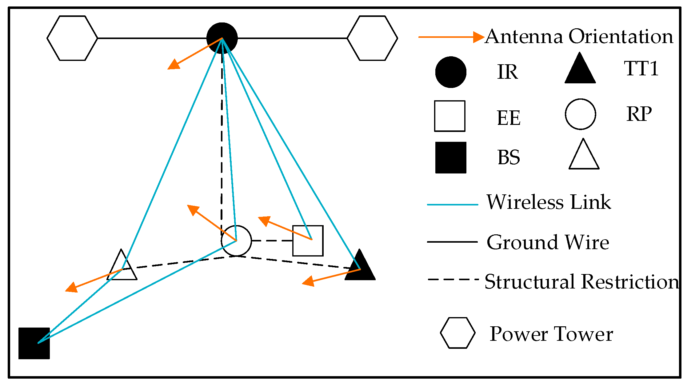
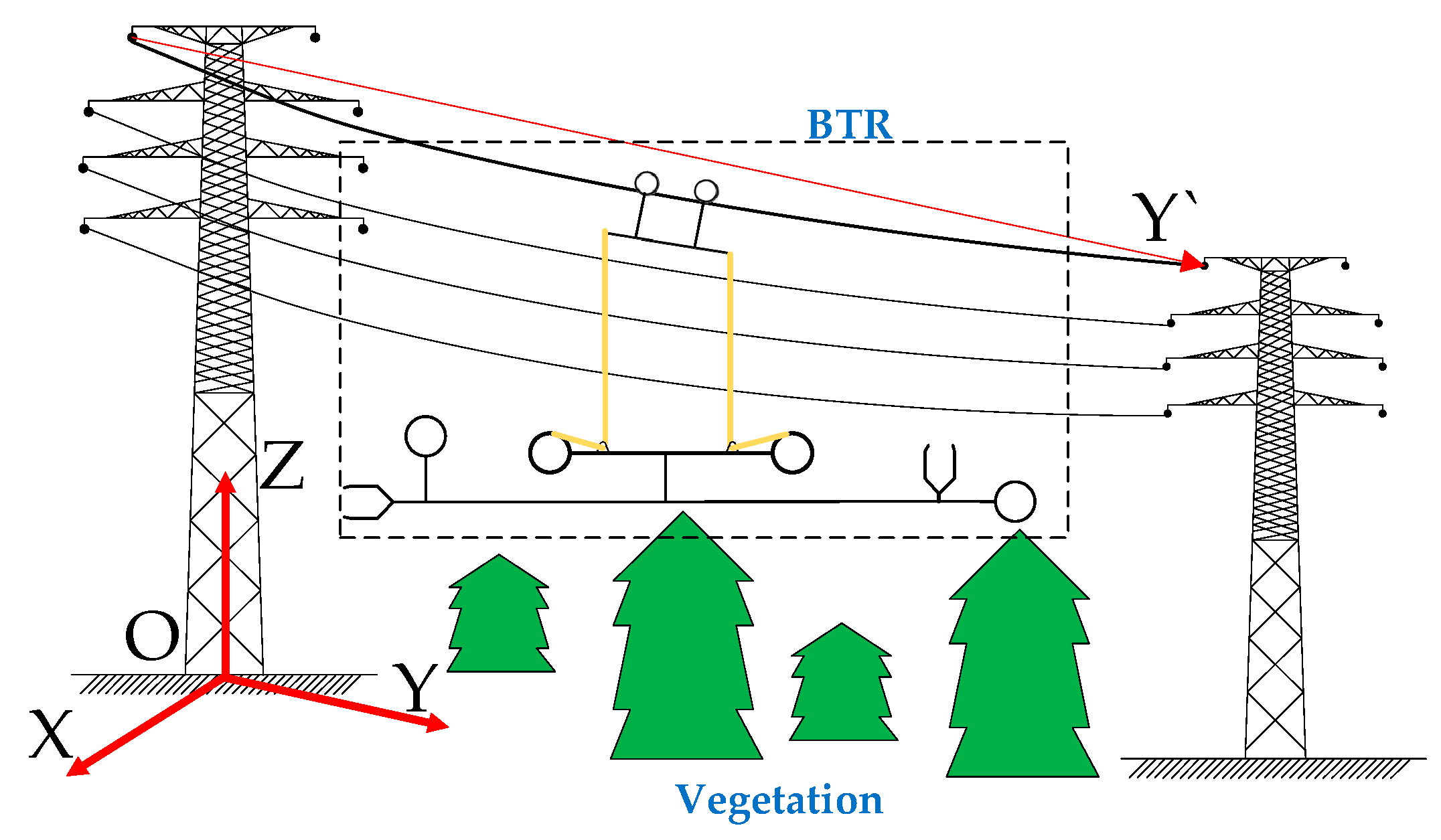
The DBTRN model is established in this section, which is shown in Figure 3. The BTR and its components are deployed along a ground wire of a single span between two power towers. The IR is deployed along the ground wire; the other components are deployed in the three-dimensional area in the transmission line corridor of a single span. The communication nodes in the DBTRN include the IR, BS, Rotary-Lifting Platform (RP), Trimming Terminal 1 (TT1), Trimming Terminal 2 (TT2), and Emergency Equipment (EE). Among these nodes, the IR, RP, TT1, and TT2 correspond to the sub-robots of the BTR; the EE is deployed inside the RP to restart the RP in case of emergency; lastly, the IR, RP, TT1, TT2, and EE are mobile nodes, while the BS is static. All the nodes above are equipped with directional antennas. In Figure 3, structural restriction represents the structure of the BTR that limits the distance and angle of some pairs of nodes. For instance, the distance between TT1 and TT2 is a fixed value owing to structural restriction, and the RP is directly below the IR, even though the distance is adjustable between the IR and the RP. These nodes form a wireless sensor network with dynamic network topology. The DBTRN has the following properties.
  • The nodes of the DBTRN have heterogeneous communication capabilities due to the movement of each node; directional antennas make the communication capabilities of mobile nodes change over time and space.
  • Each node regulates velocity (speed and direction) according to the location of target branches, surroundings, maximum motion range, etc.
  • The data delivered by these nodes have heterogenous capacity, packet delivery ratios, and network delay requirements.

3.2.1. Variable Distances between Nodes

In the DBTRN, the RSS of each node is one of the metrics of network performance. The major parameters affecting the signal strength include the distance between pairs of nodes and the orientation of the directional antenna equipped on each node. When the BTR is operating in a span, the distances between the BS and other nodes of the multi-robot system, and the distances of pairs of mobile nodes in the multi-robot system, are variable. In this section, taking the BTR working in a span as an example, the distances between the BS and mobile nodes in the multi-robot system, and the distances between pairs of nodes are discussed.
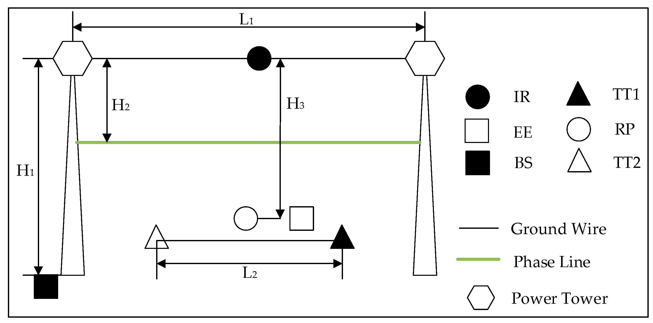
By querying the line parameters table provided by the local electric department, the distance between two towers, the maximum height of the tower, the height of the ground wire, and the height of the phase line can be obtained. The BS is placed at a point on the ground within the span, the coordinates of which are determined by the terrain between towers. The distance between the IR and other mobile nodes can be determined by the workspace and structural design of the BTR. The distribution of the DBTRN in a span is shown in Figure 4. Here, L1 denotes the horizontal distance between the two towers; L2 is the distance between the two trimming terminals; H1 is the height of the tower; H2 is the height difference between the ground wire and the phase line; and H3 is the height difference between the node IR and other sub-robots in the multi-robot system. Among these parameters, L1, L2, H1, and H2 are determined by the fixed parameters of the transmission lines, towers, terrains in the span, and the structure parameters of the BTR. In addition, H3 is determined by the locations of the trees and branches around the phase line and the length of the insulation ropes.
Table 1 gives the range of each distance. The table also describes the range of distances between pairs of mobile nodes derived from the parameters presented above.

3.2.2. Mobility Model of DBTRN

The distances between the nodes affect the network performance of the DBTRN network. When the BTR detects and trims the branches in a span between two power towers, the distances between the BS and the other nodes will change. Also, distance is a vital parameter affecting network performance. To quantify the distances between nodes, this section relies on the mobility model of the DBTRN to calculate the position coordinates of each node.
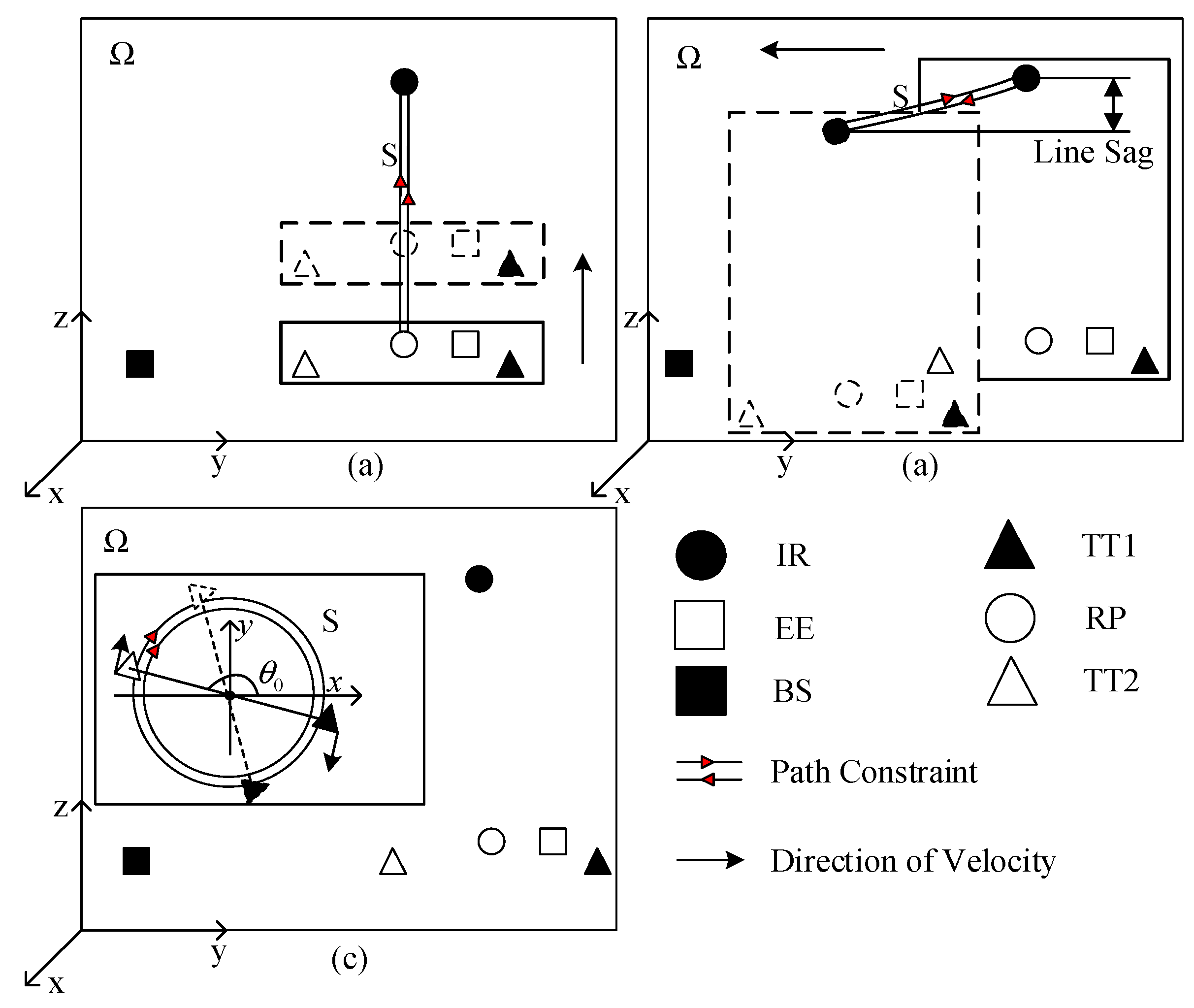
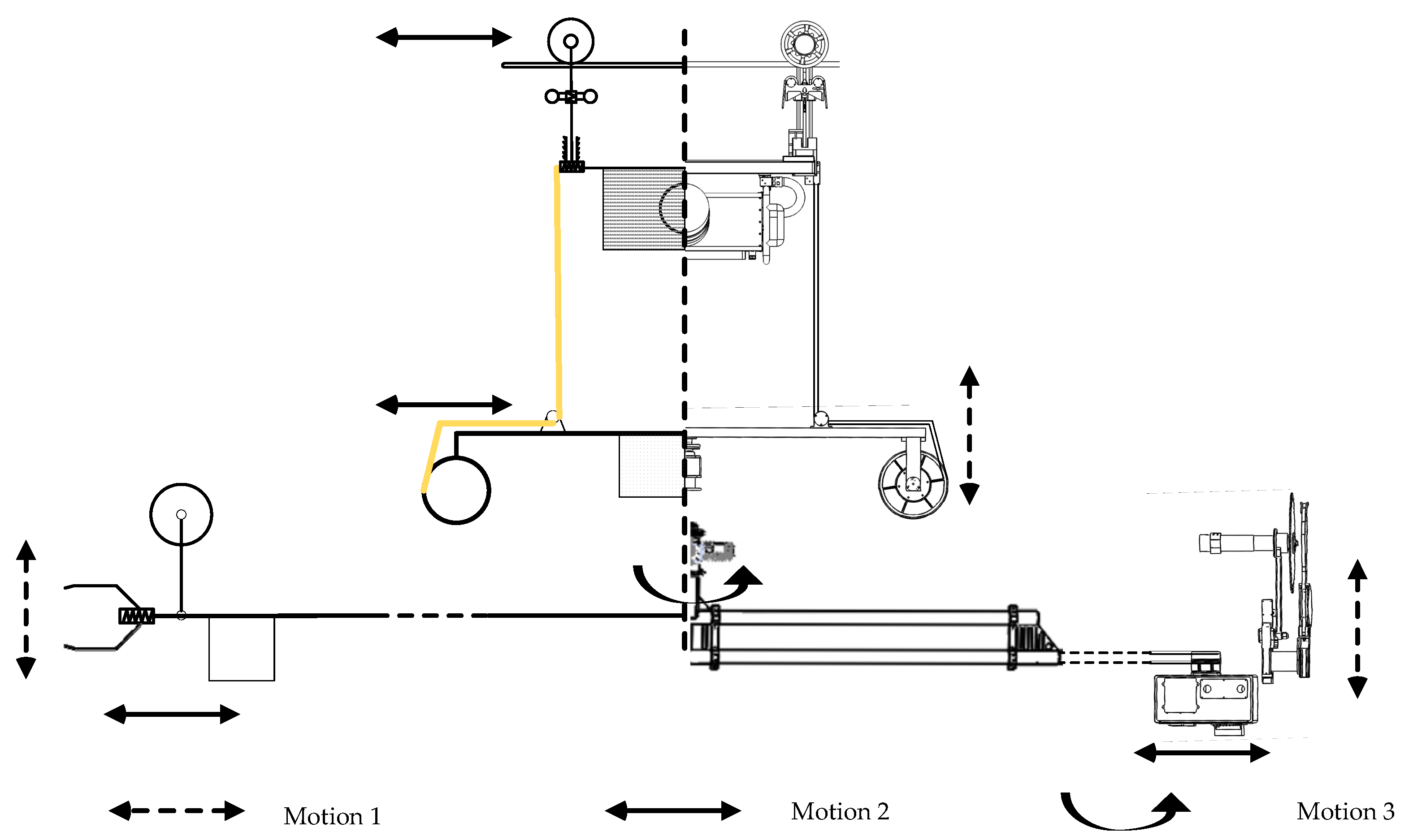
In the network model, all the nodes are deployed in a three-dimensional space in the transmission line corridor. Generally, the purpose of the BTR after it is deployed in the transmission line corridor is to find hazardous tree branches and carry out the trimming task. The mobility model of the BTR is designed and analyzed from its practical application. Motions of mobile nodes when the BTR is approaching target branches and performing trimming tasks can be classified as simple motions. The simplified BTR and mobile nodes’ movement rules are presented in this section. The movement of nodes in different motions is given in Figure 5.
  • Motion 1. The RP, EE, TT1, and TT2 move in the vertical direction, which corresponds to the lifting or the declining of the executing mechanisms. The path constraints of these nodes are vertical lines, as shown in Figure 5a. In this motion, these above nodes get a velocity vector ( 0 , 0 , ν z ) , where v z ( v m a x , v m a x ) .
  • Motion 2. The IR walks along the ground wire, and all mobile nodes move in the horizontal direction with the IR; these nodes get a velocity vector ( 0 , v y , 0 ) , where v y ( v m a x , v m a x ) . The path constraint is the ground wire. In addition, each node decline is caused by the line sag of the ground wire when the IR moves along the ground wire.
  • Motion 3. TT1 and TT2 rotate around the center of the RP, and the coordinate of the center is changeable. The velocity vectors of TT1 and TT2 are ( cos ( θ 0 + ω t ) , sin ( θ 0 + ω t ) , 0 ) and ( cos ( θ 0 + ω t ) , sin ( θ 0 + ω t ) , 0 ) , respectively, where θ 0 denotes the initial angle of the line segment of TT1 and TT2, which is positive on the X-axis; ω is the rotational angular velocity of the two nodes, and ω ϵ ( ω m a x , ω m a x ) ; t is time, as the two terminals have been rotating. During Motion 3 of the performing BTR, the path constraint of TT1 and TT2 is a circle, which is shown in Figure 5c.
  • Motion 4. All the mobile nodes stay stationary while the BTR is trimming tree branches. When the BTR is performing a trimming task, only one joint of one trimming terminal is moving. Furthermore, mobile nodes determined by the locations of nodes are dynamic until the trimming terminal finishes the trimming task or the BTR finds it unlikely to trim hazard tree branches. In this motion, the trimming task is performed by TT1.
  • Motion 5. All the mobile nodes stay stationary to trim tree branches. In this motion, the trimming task is performed by TT2.
In Figure 5, Ω denotes the maximum range of mobile nodes, which is a three-dimensional area that is determined by the safety distance of the energized conductors on the transmission line, the length of span, and the height of the power tower. The path constraint is determined by the ground wire and the structural restriction of the BTR.
The initial positions of each node are known, which are determined by fixed parameters such as the height of the power tower, the terrain around the power tower, the weight of the BTR, the length of the span of the BTR, and the structural size of the BTR. At the beginning of the trimming task, all of the noted parameters and angle of the directional antennas are set.
Equation (1) shows a simplified calculation of the positions of nodes in the DBTRN, in which ( x i ( t ) , y i ( t ) , z i ( t ) ) are the coordinates of node N i , the coordinate system is shown in Figure 6, and denotes a set of variables that determine the initial positions of nodes in the DBTRN. is a set of motions and durations of motions of mobile nodes before time t .
N i ( x i ( t ) , y i ( t ) , z i ( t ) ) = G ( , )

3.2.3. RSS Mathematical Model

The packet delivery ratio and network delay are major concerns of the WSNs. A high RSS generally corresponds to high packet delivery ratio and low network delay [36,37]. At low signal strength, the packet delivery performance is easily affected by the significant variability caused by the receiver performance and noise in the environment. Accordingly, the estimation and prediction of the RSS is vital to estimate and improve the network performance. A method is proposed in this section to improve the network performance of the DBTRN, which is achieved by assessing the RSS value of each mobile node from other nodes before the BTR performs a certain motion.
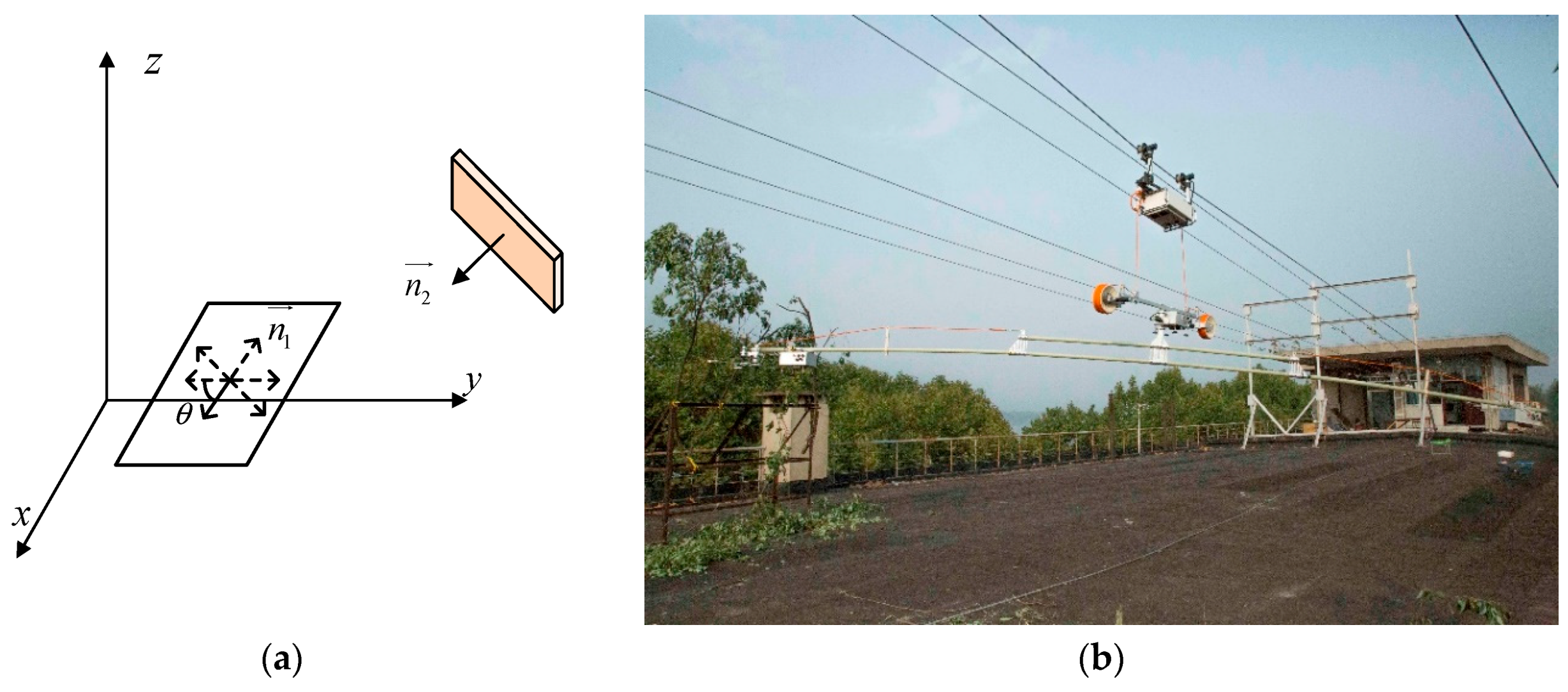
Each node in the BTR is outfitted with a directional antenna to enhance the signal strength. It makes the quantification of the RSS more complex. The RSS value is an estimate of the signal energy at the receive node [23], which is related to the antenna gains of the receiver node and the transmitter node. As mobile nodes in the DBTRN perform a motion, changes to the antennas’ angles of arrival and the distance between nodes cause changes of antenna gains, which change with a resulting change in the signal energy level at the receiver. Thus, to ensure a good packet delivery performance, wireless nodes should predict the RSS value of each mobile node before the BTR starts to perform a motion. Assume that N i ( x i , y i , z i ) denotes the coordinate of the node N i , and n i = ( a i , b i , c i ) is the unit normal vector of the antenna plane. The RSS between any pair of nodes N i and N j can be calculated by the equations below.
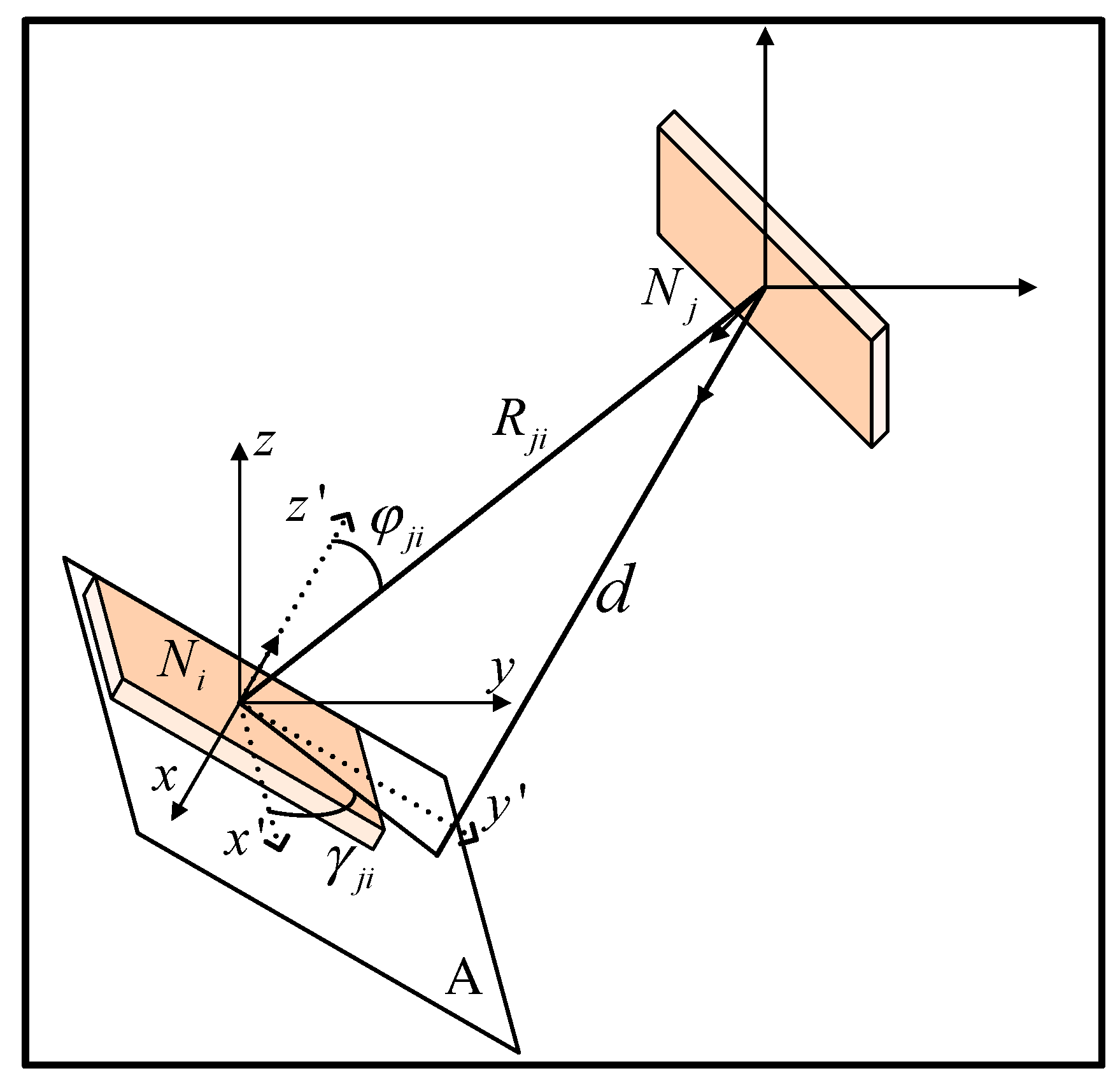
Two directional antennas of nodes with different antenna orientations are shown in Figure 7. R j i denotes the distance between node N j and node N i ; d is the distance from node N j to the antenna plane A ; φ j i is the angle measured off the Z-axis; and γ j i is the angle measured counterclockwise off the X-axis. φ j i and y j i are correlated with the positions of node N j and node N i , as well as the initial angles between directional antennas in a geodetic coordinate system. The variables above can be determined by the coordinates of nodes and the unit normal vectors of antenna planes, as calculated by Equation (2) to Equation (5).
R j i = ( x j x i ) 2 + ( y j y i ) 2 + ( z j z i ) 2
d = a i · ( x j x i ) + b i · ( y j y i ) + c i · ( z j z i )
cos φ j i = d R j i
sin γ j i = y j y i R j i 2 d 2
The gain of an antenna is related to the directivity and radiation efficiency, and the directivity is determined merely by the radiation pattern of an antenna [38]. In this study, the radiation efficiency is considered a constant, and the antenna gain is expressed in Equation (6), where φ j i denotes the angle measured off the Z-axis, and γ j i is the angle measured counterclockwise off the X-axis. φ j i and γ j i are related to the positions of node N j and node N i , and the initial angles between directional antennas in a geodetic coordinate system.
G j i = F ( φ j i , γ j i )
P j i = ( P L F ) · P i G j i G i j c 2 ( 4 π R i j f ) 2
The RSS value can be calculated by Equation (7), which is the derivation of frees transmission [39], where P j i denotes the RSS value of node N j received from node N i , P L F is the polarization loss factor (PLF) which describes power loss due to the inconsistency in polarization between a pair of antennas, G j i is the antenna gain of node N j in the direction of the antenna of node N i , G i j is the antenna gain of node N i in the direction of the antenna installed at node N j , c is the propagation speed of electromagnetic waves in vacuum, R j i is the distance between node N i and node N j , and f is the frequency of the electromagnetic waves.
Combining Equations (1) to (7), the RSS of node N j received from node N i at time t can be calculated. Equation (1) shows the calculation of coordinates of a node at time t ; Equations (2) to (7) calculate the RSS value by the coordinates of nodes and the unit normal vectors of the current direction of the antenna plane. Based on the above equations, the expression is then simplified. The RSS of node N j received from node N i can be calculated by Equation (8), where P j i ( t ) denotes the RSS of N j received from N i , is a set of variables that determine the initial position of nodes in DBTRN, is a set of motions and durations of motions before time t , and n i = ( a i , b i , c i ) is the unit normal vector of the antenna plane.
P i j ( t ) = G 1 ( , , n i , n j )

3.2.4. Discrete Time Mathematical Model

An optimal solution of how to determine the best network topology is proposed in this section for points at which the BTR is approaching target branches or trimming hazard tree branches. The solution is performed based on the statistical methods of RSS and motions of the BTR.
For the DBTRN, as the nodes move to perform trimming tasks, the network topology is unreliable and varying constantly. The movement of nodes not only changes the distances between pairs of nodes, it also changes the angle of arrival of directional antennas. Both variables above change the RSS of each node, which may significantly affect the packet delivery performance between nodes [36,37]. In order to meet the requirements of the mobile wireless nodes (RP, IR, TT1, TT2, and EE) to transmit information to the BS, this section draws on references [25,26,27], and introduces graph theory to describe the network model. Additionally, the mathematical model is designed for a mobile node in the DBTRN to find an optimal path to the BS.
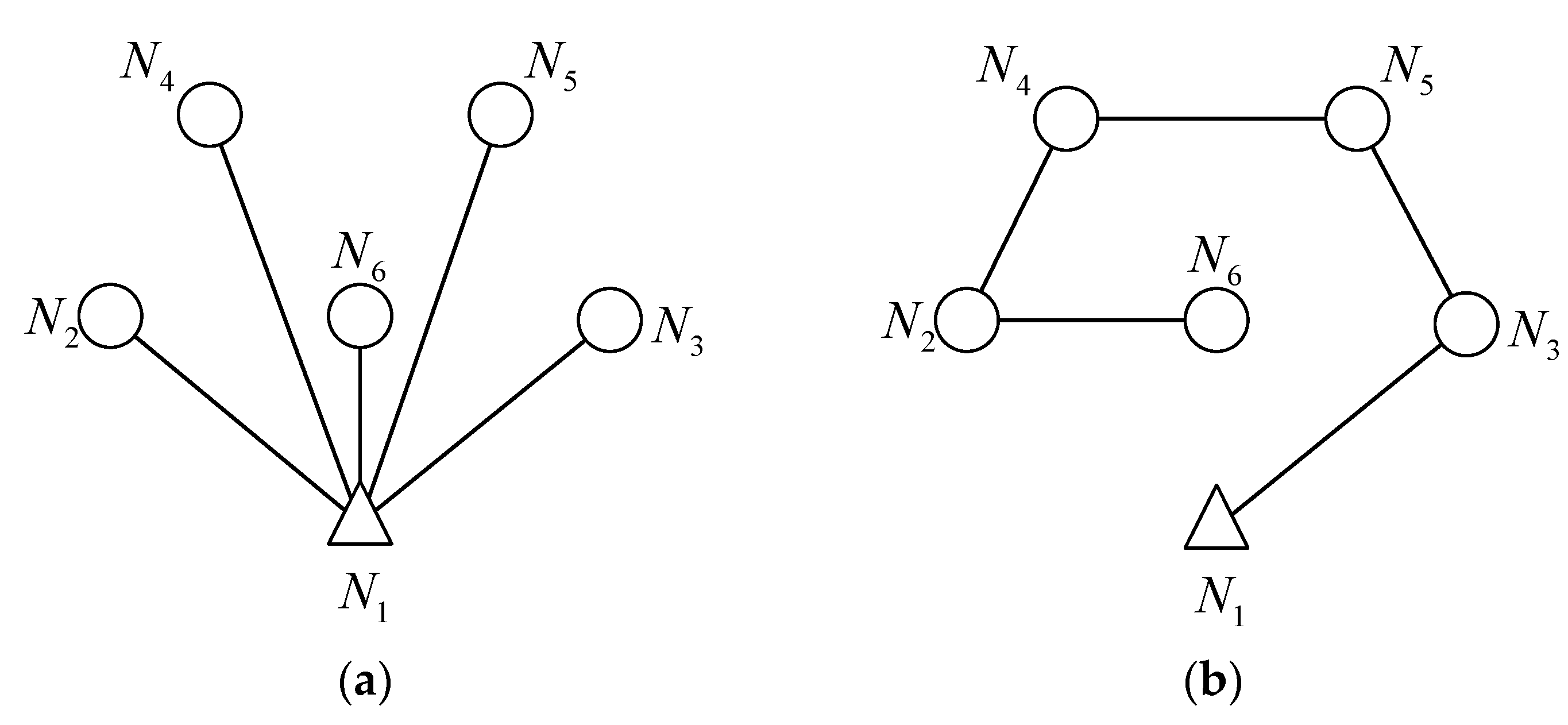
In the network mathematical model, the nodes and the information of the network can be represented by graph G ( t ) = ( V , E ) at time t , where each vertex represents the corresponding node in the DBTRN with a unique ID. The graph G ( t ) is illustrated in Figure 8. An edge represents a wireless link between vertices if the corresponding nodes are within the transmission range of each other. At time ( t + 1 ) , graph G changes, which may be represented by graph G ( t + 1 ) = ( V , E ) , and G ( t + 1 ) represents an extension of G ( t ) . All the information of the network is contained in Graph G . Besides, the weight function a i j ( t ) of each edge in graph G is calculated by Equation (9). Equation (9) expresses the law of weight variation over time. The network changes the network topology based on the weight calculation of each wireless link. Node N i decides to be connected to N j or disconnected with N j based on a i j ( t ) .
a i j ( t ) = α g i j ( t ) + β m i j ( t )
The equation above illustrates the calculation of the weight of the wireless link between node N i and node N j at time t , where a i j ( t ) denotes the weight of the wireless link between pairs of nodes, g i j ( t ) is the parameter related to RSS, which corresponds to the RSS between node N i and node N j . m i j ( t ) is the correlation coefficient between node N i and node N j when the BTR is performing a motion at time t . In Equation (10), the objective function of the network mathematical model is proposed. As shown in the description of Equation (10), the weights of all the possible paths from node N i to node N j are compared. This comparison ensures that node N i connects to node N j with the maximum weight of the wireless links, which leads to a high packet delivery ratio and low network delay. a i k i ( t ) denotes the weight of the wireless link between node N i and node N k i , where node N k i can be a relay node or does not exist; if node N k i does not exist, that means that node N i connects to node N j directly. The constraints of the wireless links between nodes are shown in Equations (11) and (12). Equation (11) demonstrates that the number of relay nodes of the path cannot exceed the number of nodes in the network except for those in node N i and node N j . n denotes the number of relay nodes, while N is the number of nodes in the DBTRN. Equation (12) shows that the relay nodes are different in the process of a packet delivering from N i and node N j .
Objective function:
max ( a i k 1 ( t ) + a k 1 k 2 ( t ) + + a k n j ( t ) ) n + 1
Constraints:
n N 2
N i k i k j N j

3.3. Dynamic Network Topology Control Strategy (DNTCS)

This section introduces the DNTCS. The DNTCS primarily aims to provide the DBTRN with the most suitable network topology. The DNTCS is a network topology control strategy that is designed for the DBTRN, which is unique regarding its mobility model, QoS requirement, and operational style. The BTR mainly aims to achieve the specific goal of detecting and trimming the branches that threaten the transmission line security. Accordingly, the goal of the DNTCS is to allow the DBTRN to have the best network performance in the process of approaching and trimming branches. In Section 3.2.2, the process of the BTR approaching and trimming branches is simplified to a few simple motions, and as shown in the description in Section 3.2.3, every motion of the BTR may result in the poor network performance of the DBTRN. Thus, the DNTCS in this study is based on the DBTRN model and the motion model of the BTR to make the BTR more efficient in the task of detecting and trimming branches.
To achieve the above objectives, the DNTCS follows the ideas below:
  • Estimate the weight value of each wireless link accurately in the DBTRN before each motion of the BTR is performed, which will ensure the continuity of the BTR during the execution of the motion. It is stipulated that the DBTRN is not allowed to switch the network topology when the BTR performs a motion, because the initialization time of the switching network topology is uncertain. This indefinite time will cause unpredictable errors in the BTR’s execution. Accordingly, switching the topology of the DBTRN before each motion of the BTR is important. However, this will definitely result in taking BTR motions into consideration when the weight of wireless links is calculated. In this section, the BTR motions are quantified and modeled to make the calculation simpler.
  • The principle for switching the topology is decided by the weight value of each wireless link in the DBTRN. Since the network topology consists of a set of wireless links, the network topology of the DBTRN is determined by selecting a suitable wireless link between a mobile node and the BS.
The DNTCS primarily seeks to confirm a proper network topology before the BTR start a motion, which is based on the prediction of the weight of each wireless link, a i j ( t ) . In the DNTCS, before the BTR starts a motion, the weight a i j ( t ) of each wireless link is calculated precisely. The weight a i j ( t ) is determined by the RSS-related parameter g i j ( t ) and the correlation coefficient m i j ( t ) , as expressed in Equation (9). The g i j ( t ) is determined by the RSS value of the corresponding vertex of the wireless link. g i j ( t ) is determined by the RSS of the nodes in the wireless networks [25]. When the RSS of node N i received from node N j reaches a certain threshold, P t , g i j ( t ) is equal to 1, as expressed in Equation (13). If the RSS is smaller than the threshold P t , g i j ( t ) is calculated by Equation (14). This value stresses the distance between node N i and node N j and the angle of arrivals of the directional antennas installed on node N i and node N j . For instance, if the distance between node N i and node N j is too high, or the antenna gains of node N i and node N j are relatively low, the RSS-related parameter g i j ( t ) will be small. P i j ( t ) can be calculated by Equation (8):
g i j ( t ) = 1 , P i j ( t ) P t
g i j ( t ) = l o g 10 ( P t / 1 m W ) l o g 10 ( P i j ( t ) / 1 m W ) , P i j ( t ) < P t
Another important parameter when calculating the weight of the wireless link is m i j ( t ) , which denotes the correlation coefficient between node N i and node N j as the BTR is performing a certain motion at time t . To improve the calculation of the equations, each node needs to be numbered. The sequential representation of nodes is shown in Table 2.
m i j ( t ) is valued based on the necessity of being monitored when the BTR is performing motion l , as expressed in Equation (15).
L i j = [ 1 1 1 1 1 0 1 0 0 0 1 0 1 0 0 1 0 1 0 0 1 1 1 1 0 1 1 1 0 1 ] , K i j = [ η η η η η 1 η η 1 η 1 η 1 η η 1 η η 1 η 1 η η 1 η η 1 η 1 η η η η η 1 η η η η 1 η η ]
In Equation (15), l i j (elements of Matrix L i j ) denotes the necessity of node N i being monitored when the BTR is performing motion j . For instance, when the BTR is performing motion 3, the IR should not be monitored for being static, so the necessity of it equals 0. k i j (elements of matrix K i j ) is a derivative of l i j , representing the connectivity of a node in the network topology. k i j represents the connectivity of N i when the BTR is performing motion j . m i j ( t ) can be calculated by Equation (16), representing the correlation coefficient between N i and node N j .
m i j ( t ) = k i l ( t ) + k j l ( t )
Before the BTR starts to perform a motion, the motion range of mobile nodes can be calculated by the following equations. In Equation (17), D denotes the duration of the BTR performing motion l ; v i is the velocity of node N i when the BTR is performing motion l ; N i ( x i , y i , z i ) is the location before the BTR performs motion l ; Ω i D is the location of node N i when the BTR has been performing motion l for a period of D . In Equation (18), Ω i l denotes the motion range of node N i when the BTR is performing motion l ; and Ω is the maximum motion range of the mobile nodes.
Ω i D = v i · D + N i ( x i , y i , z i )
Ω i l = ( Ω i D ( 0 < D < ) ) Ω
In addition, this section combines the DNTCS with the mathematical model introduced in Section 3.2.4. Based on the mathematical model and the calculation methods presented in this study, a mobile node in the DBTRN can find an optimal path to the BS through the calculations. The weight value of each wireless link is determined by the historical information of the DBTRN, the motion to be performed by the BTR, and the location information of each node and the orientation information of the antenna. After the weight values are settled, the appropriate path from the mobile node to the BS is selected according to the objective function and constraints in Section 3.2.4. After the appropriate path from each mobile node to the BS is determined, the network topology of the DBTRN is then confirmed. The process of the optimal path solution is presented below.
  • First, check whether the necessity of the node N i being monitored equals 1 or not. If the necessity equals 1, the following steps need to be executed. If the necessity equals 0, the following steps will not be executed.
  • Second, calculate weight a i j ( t ) of the wireless links between node N i and the other wireless nodes depended on the motion range Ω i l , g i j ( t ) , and m i j ( t ) . The interval of a i j ( t ) can be obtained, a i j ( t ) [ a m i n , a m a x ] ; let a i j ( t ) = a m i n .
  • Finally, find the best path from node N i to the BS based on the objective function and constraints presented in Section 3.2.4.
After the optimal path from a mobile node to the BS is determined, the process of the proper network topology deployment is presented as follows.
  • First, set a motion that the BTR will perform in the subsequent time.
  • Second, select the optimal path from the mobile nodes to the BS if the necessity of the node being monitored in this motion equals 1.
  • Finally, the best deployment of network topology is obtained by combining the optimal paths from the mobile nodes to the BS.
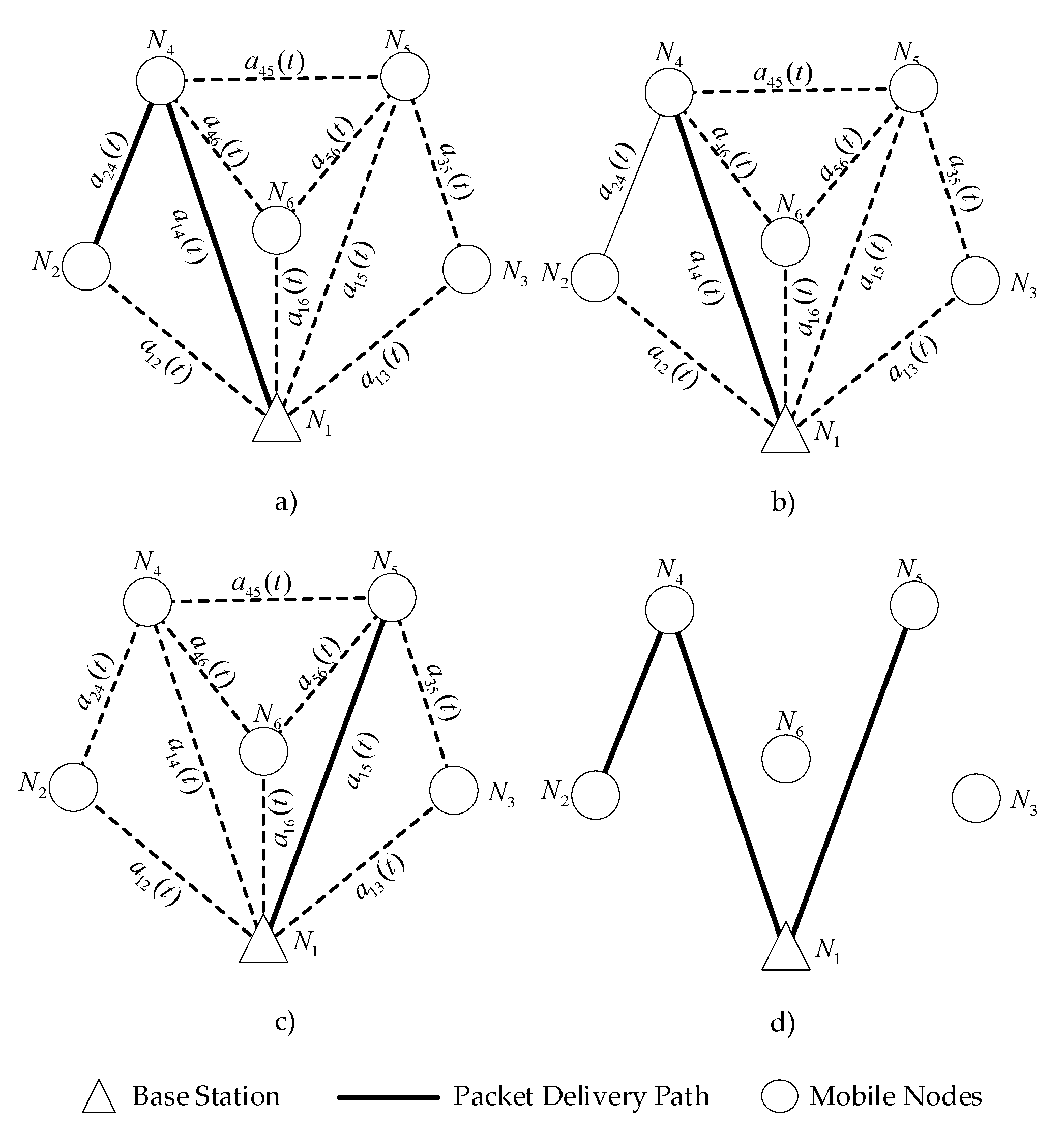
Figure 9 gives an example of the DNTCS at work. The BTR will perform motion 2 at time ( t + n ) . The information of nodes N 2 , N 4 , and N 5 must be transmitted to N 1 . The dynamic network topology is determined by the path selection from N 2 to N 4 and N 5 to N 1 . The network topology before the BTR performs motion 2 can be verified by the following steps.
  • Step 1: Calculate the weight of each wireless link in the DBTRN.
  • Step 2: Based on the calculated statistics, node N 2 , node N 4 , and node N 5 select the optimal path to the BS through the proper wireless links as shown in Figure 9a–c, respectively.
  • Step 3: The network topology of the DBTRN when the BTR performs motion 2 is determined by the optimal paths presented in Step 2, as shown in Figure 9d.
The DNTCS solves the problem of deploying the best network topology of the DBTRN before the BTR performs a certain motion, which is performed by the optimal path selection from the mobile nodes to the BS with the objective function and constraints. The DNTCS enables calculating methods of variables in the mathematical model and a method to choose a proper network topology. The Dynamic Network Topology Control Strategy (DNTCS) is represented as pseudo-code, as shown in Algorithm 1.
Algorithm 1. DNTCS
1:{path} = main (M, v)  %M: motion type, v: velocity of nodes
2:load locations  %locations of nodes before performing a motion
3:set matrix L, α, β, η
4:for(i = 2: N)  %N: number of nodes in the DBTRN
5:{predict locations(a)
6:connectivity update(b)
7:for (0 < j < i)
8:{update P i j (c)
9:update g i j (d)
10:update m i j (e)
11:update a i j }(f)
12:path N i -BS ()}
13: path
Algorithm 1 runs iteratively for increasing N values, where N is the size of a node set in the DBTRN. Table 3 shows the time complexity of the main steps of Algorithm 1.
The function path N i –BS is designed to compare the weights of all the possible paths from node N i to BS; the time complexity of this function using the brute force algorithm is shown in Equation (19). The brute force algorithm is a general technique that consists of enumerating all the possible candidates for the objective function and selecting the best solution to satisfy the problem statement [40]. Obviously, due to the time complexity of the function path N i –BS, the application of the DNTCS to the DBTRN will be extensively affected as the value of N increases.
T ( N ) = i = 0 N 3 A N 2 i
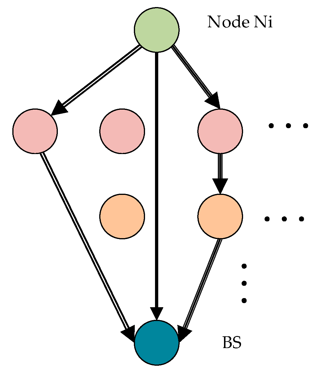
We use the ant colony optimization (ACO) algorithm to optimize the objective function in a short execution time. The paths of the objective function are shown in Figure 10; each ant tries to find a path from node N i to the BS. The other ants follow one of the paths at random, laying pheromone trails, which denotes the average weights of the paths.
ACO is a biologically inspired technique simulating the foraging process of social insects [41,42]. ACO uses a graph G ( t ) = ( V , E ) . V denotes the nodes in the DBTRN, and E denotes the undirected edges, respectively. Two nodes N i , N j V are neighbors, and ( N i , N j ) E . Each edge is annotated with weights. A path is a sequence of nodes and edges between a source and destination. The objective of ACO is to find a path between the source and destination with minimal weights.
To solve the objective function in Equation (10), a path-selecting algorithm for the DBTRN based on ACO is proposed by selecting the edge with the maximum weight when an ant arrives at a node. A complete iteration of the optimized path-selecting algorithm based on ACO consists of the following steps:
Step 1: Initialization
During initialization, each edge of graph ( N i , N j ) E in graph G is associated with the initial pheromone weight a i j , as shown in Equation (20):
a i j = a 0 , ( N i , N j ) E
Step 2: Construct a probabilistic solution
Constructing a path is based on stepwise estimation for each edge ( N i , N j ) according to Equation (21), where Β i k denotes the neighbors of the k-th ant at node N i , and τ is a parameter that controls the influence of a i j .
p i j k = { a i j τ l Β i k a i l τ N j Β i k 0 N j Β i k
Step 3: Pheromone update
After the ant arrives at the destination node, a path is found. On this path, loops are eliminated by checking whether a path includes the same node. Additionally, the ant updates the pheromone level for all the edges on the path. The new pheromone is updated according to Equation (22), where Δ a k is the amount of pheromone deposited by the k-th ant.
a i j = a i j + Δ a k
Step 4: Pheromone evaporation
In order to make the algorithm robust in dynamic networks, the pheromone needs to be evaporated over time for all the edges. The pheromone is decremented over time, as shown in Equation (23), where ρ ( 0 , 1 ] is the pheromone evaporation coefficient.
a i j = ( 1 ρ ) · a i j , ( N i , N j ) E
The algorithm converges if a solution reaches a certain quality level or if no more changes are performed. The pseudo-code of the optimized method based on ACO is shown in Algorithm 2.
Algorithm 2. Optimized Method
1:path Ni-BS ( a i j )
2:graph_edges = a i j
3:construct objective functions
4:initialize pheromone trails and parameters
5:set iteration number M
6:for (i = 1: M)
7:{construct a solution
8:update local pheromone
9:compute solution quality}
10M = M + 1
11Path = candidate to be optimal solution
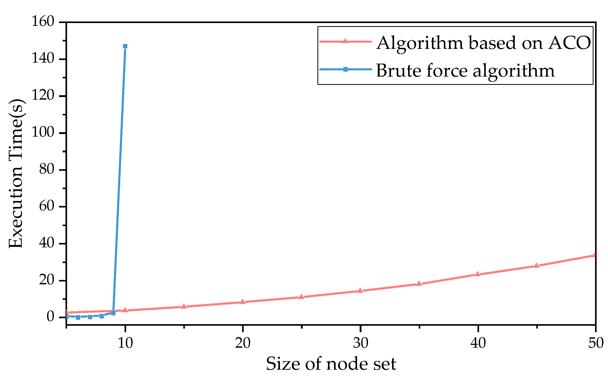
Since the size of the node set in the DBTRN is not specified, the algorithm runs iteratively for increasing N values and has a run time of O ( N 2 ) , where N is the size of the node set of the DBTRN. In comparison, a brute force algorithm would take O ( ( N n ) ) . Compared with a traditional algorithm, the path-selecting algorithm based on ACO can reduce execution.

4. Experiment and Results

This section uses the BTR prototype developed by Wuhan University to achieve the results of the DNTCS in the DBTRN. The results are achieved by three experiments, namely the RSS mathematical model experiment, the experiment for testing the DNTCS applied to the DBTRN, and the experiment for testing the DNTCS in other networks. The RSS mathematical model experiment was designed to verify the RSS mathematical model presented in Section 3.2.3. Experiments for testing the DNTCS were designed to obtain the network performance of the DBTRN when the DNTCS was used. Furthermore, the effects of the DNTCS applied in other networks were obtained by experiments.

4.1. Results for RSS Mathematical Model

RSS prediction is an important part of the DNTCS. To verify the RSS mathematical model presented in Section 3.2.3, the BTR and the BS with directional antennas were used in this experiment. The BTR was deployed at a fixed point on a simulated transmission line, which was built on the roof of a building in Wuhan University, as shown in Figure 10b; the BS was static, and the direction of its antenna was adjustable.
In this experiment, a geodetic coordinate system was adopted; different RSS values were recorded as the plane normal vector of the directional antenna changed. As shown in Figure 11a, n 1 denotes the plane normal vector of the directional antenna of BS, and n 2 is the plane normal vector of the directional antenna of IR. To make the measurement concise and clear, the plane normal vector of the directional antenna of BS was parallel to the XOY plane of the geodetic coordinate system. Ten different RSS values of the BS received from the IR were recorded depending on the different plane normal vectors of the directional antenna. A comparison between the experimental and theoretical values is shown in Figure 12. θ represents the angle between the plane normal vector and the positive X-axis; theoretical values are calculated by Equation (7), and the measured values are the average values of each of the 10 recorded values.
The errors between the theoretical values and recorded values are shown in Table 4, and the analysis and discussion of test errors are given in Section 5.1.

4.2. Results for Optimized Path Selecting Algorithm

The optimized path-selecting algorithm is an important part of the DNTCS to solve the objective function in Equation (10). The execution time of path selecting affects the efficiency of the trimming task of the BTR. To investigate the execution time of the path-selecting algorithm based on ACO, experiments were performed in this section. In the experiments, comparison was performed on the effect of the node set of the DBTRN when the brute force algorithm and algorithm based on ACO are adopted. The proposed method is implemented in Matlab; the experiments are conducted on a laptop with 2.4 GHz CPU and 8 GB memory running Windows 10. The main ACO initialization parameters are configured as follows: τ = 1 and ρ = 0.5 . Figure 13 shows the execution time of the brute force algorithm and path-selecting algorithm based on ACO, where the ACO uses 200 ants and 20 iterations.
As shown in Figure 13, the execution time of the algorithms above increases with the growth of size of the node set. When the size of the node set exceeds 10, the solution candidates of the best paths exceed the upper bound of the memory. Therefore, the brute force algorithm is not applicable for the path selecting when the size of the node set exceeds 10. Compared with the brute force algorithm, the path-selecting algorithm based on ACO takes less time, and it is suitable for the path selecting of the DNTCS. Additionally, the optimized path-selecting algorithm based on ACO is capable of maximizing the objective function in less time. Since the execution time of the path selection takes less than 30 s, the normal trimming of the BTR will not be affected by the execution time of the algorithm.

4.3. Experiment and Results for DNTCS

4.3.1. Experiment Explanation and Parameters

This section describes experiments to investigate the variation of network performance when the DBTRN adopts the DNTCS. The experiments were performed in a single span of a 220-kV high-voltage transmission line, and the BTR underwent relevant 220-kV AC high-voltage breakdown and withstand tests in Jilin Province, China. Figure 14 suggests that the ground line, phase lines, and trees are abbreviated as E, F, and G, respectively. Moreover, A, C, and D are the abbreviations of IR, TT1, and TT2, respectively. It is noteworthy that RP and EE are too close to distinguish from the figure, so C refers to the abbreviation of RP and EE. The default parameters of the single span, movement rate of the mobile nodes, and antenna orientations are listed in Table 5.
In this experiment, the BTR approached the target branches in a single span after it was assembled. As the BTR approached the target branches, the approaching of the BTR is split into several motions. The different motions of the BTR are shown in Figure 15. In motion 1, the RP, EE, TT1, and TT2 moved in the vertical direction, which corresponded to the lifting or declining of the executing mechanisms. In motion 2, the IR walked along the ground wire, and all the mobile nodes moved in the horizontal direction with the IR. Two trimming terminals (TT1 and TT2) rotated around a fixed point in motion 3. Figure 5 shows the mobility of each node when the BTR performs different motions. According to the motions of the BTR, the experiment was performed in different scenarios. The scenarios are presented below.
Scenario 1. The BTR performs motion 1; the RP, EE, TT1, and TT2 are lifted in the vertical direction, and the IR remains static. The RP and EE are responsible for receiving commands from the BS in the wireless network. The RP choose to start the motion or stop the motion according to the messages received from the BS; the EE must be reachable for the BS for any emergency in which the RP is out of control. Also, TT1 and TT2 can easily trim the target branches if they are able to communicate with the BS.
Scenario 2. The BTR performs motion 2; the IR walks along the ground line, and all of the other nodes follow the IR. The IR receives messages from the BS. To easily sensor the location of the target branches, TT1 and TT2 must be reachable for the BS.
Scenario 3. The BTR performs motion 3. The rotating mechanism works; TT1 and TT2 rotate around a fixed point on the rotary platform. The mobile node RP receives messages from the BS to decide when to start the motion or stop the motion. This scenario is separated into two scenarios including Scenario 3.1 and Scenario 3.2. In Scenario 3.1, images and videos from TT1 and TT2 are not transmitted to the BS. In Scenario 3.2, TT1 and TT2 transmit images and videos to the BS, and the BS decides to send a command to stop the rotating mechanism according to the images and videos transmitted from TT1 and TT2. In these two scenarios, TT1, TT2, RP, and EE must be monitored.
To compare with the DNTCS, two other fixed topologies are deployed. Experimenting with the fixed topologies presented above implies that the DBTRN network topology is not optimized by the DNTCS when performing these motions. Two fixed topologies are classified into topology 1 and topology 2. Topology 1 uses a star topology, which is similar to the tree-based topology in WSNs and centralized communication architecture in UAV networks [16,43]. Topology 2 uses a chain topology; the chain topology is a commonly used Chain-based topology in WSNs, which are all connected with each other along a chain [12]. The implementation of the fixed topologies of the DBTRN is illustrated in Figure 16.
The experiments primarily aim to collect information about the network performance of each mobile node when the BS is communicating with it under different topologies. For this end, the experiments adopted a ping command from the BS to each mobile node. The ping command is used to test the reachability of a mobile node in the DBTRN network. It measures the Round-Trip Time (RTT) for each message sent from the BS to a mobile node in the DBTRN that is echoed back to the BS. It is operated by the BS sending Internet Control Message Protocol (ICMP) echo request packets to the mobile nodes and waiting for an ICMP echo reply. The ping command reports the packet loss rate, and a statistical summary of the results, e.g., the minimum, maximum, and mean round-trip times [44]. The RTT can be expressed by a function of network delay [45].
The ping statistics from the BS to each mobile node under different deployments of network topologies when the BTR approaches target branches were recorded. A comparison was performed on the ping statistics for fixed topologies and the dynamic topology deployed by the DNTCS.

4.3.2. Performance Metrics

The packet loss rate and network delay—the indicators of DBTRN network performance—affect the efficiency and success rate of the BTR execution. To better evaluate the network performance of the DBTRN adopting fixed topologies and the DNTCS, the packet loss rate and network delay are graded in this section.
The real-time requirement of the BTR for the packet loss rate is that the packet loss rate is not allowed to affect the normal execution of the BTR actions and data transmission, e.g., instructions, images, and videos. According to the performance metrics presented in [46,47], the packet loss rate requirement of the DBTRN is graded, as listed in Table 6.
The network delay requirement of the DBTRN is determined by the structure design and fault tolerance of the BTR. Here, we take a specific motion of the BTR as an example to explain the effect of the network delay on the execution of the BTR motions. First, we assume that the BTR is performing motion 2, which was presented in Section 3.2.2. At time T , the trimming terminal detects hazard branches. At time ( T + T 1 ) , images and videos are transmitted to the BS. At time ( T + T 1 + T 2 ) , the commands to stop motion 2 are transmitted by the BS. At ( T + T 1 + T 2 + T 3 ) , the commands arrive at the mobile node. ( T 1 + T 3 ) can be replaced by the RTT of a packet. The network delay requirement of the DBTRN is expressed in Equation (24):
v · R T T S
where v denotes the velocity of the mobile node when performing a motion, and S is the maximum value of error that the mobile node can bear. S is determined by the structural design and fault tolerance of the BTR. Thus, we have the following requirements for RTT when operating the BTR based on the structural design of the BTR and the experience of operating the BTR.
To better express the RTT from the BS to a mobile node, the following parameters are used: minimum RTT, maximum RTT, average RTT, and standard variance of RTT. These parameters are graded in Table 6.

4.3.3. Results

This section studies the network performance differences between the DBTRN with DNTCS and the DBTRN with fixed network topologies. The experiment is classified into different scenarios. In each scenario, the network performance of the DBTRN is represented by recorded statistics regarding the packet loss rate and network delay, and the network delay is represented by the RTT of a packet from the BS and mobile nodes. The results of the experiment are shown in Figure 17, Figure 18, Figure 19, and Figure 20. In each figure, the packet loss rate and RTT are shown in (a) and (b) of the figure, respectively, and (c) shows the network performance of the mobile nodes after normalization. The normalized standards are listed in Table 6. Furthermore, in each figure displaying the results, I, II, III, IV, and V denote the packet loss rate, minimum RTT, maximum RTT, average RTT, and standard variance of RTT, respectively.
For Scenario 1 of the DBTRN, Figure 17 suggests that the DNTCS and fixed topologies exhibit a similar network performance as that in Scenario 1. Compared to the DBTRN with the fixed network topologies, the DBTRN using the DNTCS has a slightly improved packet loss rate, whereas its other performances are not improved.
For Scenario 2 of the DBTRN, Figure 18 shows that all of network performance metrics of the DBTRN with DNTCS have significantly improved. Compared to the fixed topologies, each mobile node has the best packet loss rate and network delay performance when the DBTRN adopts the DNTCS.
For Scenario 3.1, the results are shown in Figure 19. For the RP and EE mobile nodes, the DNTCS exhibits the optimal network performance, and topology 1 and topology 2 are similar regarding all the network performance metrics. For the TT1 and TT2 mobile node, the DNTCS has a significantly improved packet loss rate, average RTT, and standard variance of RTT, whereas the DNTCS with fixed topologies is similar regarding its minimum RTT and maximum RTT. Furthermore, topology 1 and topology 2 are similar in all their network performances for all of the mobile nodes.
Figure 20 shows the difference of network performance in Scenario 3.2. For all the mobile nodes, the DNTCS increases the packet loss rate performance significantly; topology 1 is the worst among the three proposed topologies regarding the network performance metrics. However, for all of the mobile nodes, the maximum RTT and average RTT of the DNTCS is worse than those of topology 2, but better than those of topology 1.

5. Discussion

In this study, the experiments of the RSS mathematical model and multiple scenarios based on the DBTRN motions are performed for the DNTCS. All of the obtained results are analyzed and presented in this section.

5.1. Analysis of Results of RSS Mathematical Model

Adjusting the angle θ means changing the plane normal vector of the directional antenna of mobile node 1. As a result, the antenna gains of two directional antennas will be changed, which will affect the RSS of the BS received from the IR. Figure 12 shows that the theoretical values are bigger than the measured values. With the increase in the angle θ from −180° to 150°, the trend of the lines of the theoretical values and measured values are almost the same. Besides, the error between the theoretical values and measured values are listed in Table 4; the mean value of the error is 10.78 dBm, the standard deviation is 2.73 dBm, the minimum error is 6.11 dBm, and the maximum error is 15.31 dBm.
Considering the effect of environment variables including humidity, temperature, obstruction, and signal noise, it is reasonable that the theoretical value is bigger than the measured value. Besides, the position of the node on the transmission line can be affected by the swinging of the line, which may affect the distance between the two nodes and the arrival angles between the directional antennas of the two nodes. Accordingly, the received signal power of the BS received from the IR can be affected by the swinging of the line.
Regarding the effect of the mentioned environment variables, the received signal power calculated by the RSS mathematical model is consistent with the measured received signal power if the theoretical value of each point is not constant. Assume that the theoretical value is 10.78 dBm; the maximum error will be 4.53 dBm. As shown in Equations (13) and (14), g i j ( t ) is affected by the errors between the measured value and the theoretical value of the RSS. When the theoretical value equals the threshold of the RSS, the difference of g i j ( t ) reaches the maximum value. As shown in Figure 12, when the error between the theoretical value and measured value equals 4.53 dBm, the maximum error of g i j ( t ) equals 0.094. The maximum error of g i j ( t ) has a negligible effect on the accuracy of the DNTCS.

5.2. Analysis of Results of DNTCS

When the BTR performs different motions, the distances between the pairs of nodes and the orientations of the directional antennas installed at the nodes will affect the RSS of the wireless links. The mechanism of the DNTCS is to choose the proper wireless link from the mobile node to the BS according to the motions of the BTR. Figure 18, Figure 19 and Figure 20 show that the DNTCS significantly improves the performance of the packet loss rate and average RTT of each node in Scenario 2, Scenario 3.1, and Scenario 3.2, respectively. As for the minimum RTT, maximum delay, and standard variance of the RTT, the DNTCS is not as effective at increasing the performance of the packet loss rate and average RTT.
The BTR performs motion 1 in Scenario 1, where the executing mechanism of the BTR is lifted and declined; the height difference is not sufficiently large to significantly affect the RSS of the wireless links. Thus, the DNTCS does not obviously improve the network performance compared to topology 1 and topology 2, as shown in Figure 17. In Scenario 2, where the IR walks along the ground wire, the maximum range of its motion exceeds the distance that the BTR performs in Scenario 1. Also, the change of antenna orientation is more significant. Accordingly, the DNTCS improves the network performance better in Scenario 2 than in Scenario 1.
In Scenario 3.1 and Scenario 3.2, the DNTCS significantly improves the network performance of TT1 and TT2, as shown in Figure 19 and Figure 20. When TT1 and TT2 are rotating around a center, the rotation changes the orientations of the antennas, which significantly affects the RSS value of the wireless links. Topology 1 and topology 2 provide unstable wireless links from TT1 and TT2 to the BS, where the RSS of the wireless link is low and unstable. Introducing the DNTCS to the DBTRN significantly improves the network performance of TT1 and TT2 by choosing a better path from the mobile node to the BS, thereby greatly improving the efficiency and accuracy of the BTR. Thus, compared to the fixed topologies, the DNTCS can improve the network performance of the DBTRN and improve the efficiency and accuracy of the BTR.

6. Conclusions

This study proposes a novel method of wireless network topology control for distributed multi-robot systems e.g., the BTR using a distributed network model (DBTRN) and a topology control method in accordance with graph theory (DNTCS). The main conclusions are summarized as follows.
(1)
The DBTRN is a novel distributed wireless network system for intelligently detecting and trimming tree branches around energized transmission lines. The components of the BTR are deployed on the ground wire and in an area under the energized transmission lines. Hazard branches can be detected by images and videos transmitted from each node of the DBTRN. As the components of the BTR collaborate with each other to trim detected branches, labor intensity and unnecessary dispute have been reduced.
(2)
The proposed method primarily consists of two parts, namely the DBTRN model and the network topology control of the DBTRN. In the first part, the characteristics of the mobile nodes and the static node were introduced, and the structure of the network was presented. Subsequently, the mobility model of the BTR motions was analyzed. Next, the RSS mathematical model between pairs of nodes was proposed based on the characteristics of directional antennas installed in each node and the mobility model of the BTR motions. Finally, a mathematical model for the DBTRN was introduced in accordance with graph theory. The proposed model fully considers the structure and mobility model of the BTR, and a scheme was designed to improve the data delivery ratio and reduce network delay. In the second part, the topology control algorithm for the DBTRN was presented. The essence of the DNTCS is the optimal path selection from a mobile node to the BS. The optimal path selection is found by the weight of each wireless link, which is calculated using historic information, an RSS mathematical model, and the future motion of the BTR.
(3)
In the experiments, three experimental scenarios were performed, including the RSS prediction experiment and the effect of applying the DBTRN. According to the experimental results, the RSS mathematical model of the DBTRN can calculate the RSS between pairs of nodes accurately, which is vital for the DNTCS. According to the comparative experiment between the topology deployed by the DNTCS and fixed topologies, the DNTCS obviously improves the data delivery ratio and the network delay when the BTR performs the motions of approaching target branches. Besides, the DNTCS improves the network performance of the MRCPS, which has proven the applicability of the DNTCS.
Subsequent studies should focus on two aspects. One is that the degree to which the network links of distributed multi-robot systems change frequently in dynamic topology control; the stability of the network ought to be further analyzed. The other is to research the co-channel signal interference of the proposed multi-robot system.

Author Contributions

M.W. proposed and developed the research design, designed the experiment, collected the experimental data, performed the data analysis, interpreted the results, and wrote the manuscript. G.W. assisted with developing the research design and interpreting the results. F.F. assisted with refining the manuscript writing and coordinating the revision activities. Q.J. and W.H. assisted with designing the experiment and collecting the experiment data. Q.C. assisted with processing the experiments.

Funding

This work was supported by a State Grid Jilin Electric Power Co., Ltd. Project, China (52230015002F) and a State Grid Jilin Electric Power Co., Ltd. Project, China (JDK2015-21).

Acknowledgments

The authors wish to thank the anonymous reviewers, each of whom provided comments that made important improvements to the manuscript.

Conflicts of Interest

The authors declare no conflict of interest.

Abbreviations

The following abbreviations are used in this manuscript:
BTRBranch-Trimming Robot
WSNWireless Sensor Networks
DBTRNDistributed Branch-Trimming Robot Networks
DNTCSDynamic Network Topology Control Strategy
IRInspection Robot
RPRotary-Lifting Platform
TT1Trimming Terminal 1
TT2Trimming Terminal 2
EEEmergency Equipment
RSSReceived Signal Strength
RTTRound-Trip Time
PLFPolarization loss factor
ACOAnt colony optimization
Symbols
L1horizontal distance between two towers
L2distance between two trimming terminals
H1height of tower
H2height difference between the ground line and phase line
H3height difference between node IR and other sub-robots in the multi-robot system
v z velocity of mobile nodes in the vertical direction
v y velocity of nodes when IR walks along the ground line
θ 0 initial angel of line segment of TT1 and TT2, positive X-axis
ω rotational angular velocity of TT1 and TT2
a set of variables that determine the initial positions of nodes in the DBTRN
a set of motions and the durations of the motions of mobile nodes before time t
N i ( x i , y i , z i ) coordinate of the node N i
n i = ( a i , b i , c i ) unit normal vector of the antenna plane
R j i distance between node N j and node N i
d distance from node N j to the antenna plane A
φ j i angle measured off the Z-axis
γ j i angle measured counterclockwise off the X-axis
G i j antenna gain of node N i in the direction of the antenna installed at node N j
c propagation speed of the electromagnetic waves in vacuum
f frequency of the electromagnetic waves
P j i RSS value of node N j received from node N i
P j i ( t ) RSS of node N j received from node N i at time t
a i j ( t ) weight of wireless link between pairs of nodes
g i j ( t ) parameter related to RSS
m i j ( t ) correlation coefficient between node N i and node N j at time t
P t threshold of RSS value
l i j necessity of node N i being monitored when the BTR is performing motion j
k i j connectivity of N i when the BTR is performing motion j
Ω i D locations of node N i when the BTR has been performing motion l for a period of D
D the duration of the BTR performing motion l
Ω i l motion range of node N i when the BTR is performing motion l
Β i k neighbors of the kth ant at node N i
τ a parameter to control the influence of a i j
Δ a k the amount of pheromone deposited by the kth ant
ρ the pheromone evaporation coefficient
v velocity of mobile node when performing a motion
S maximum value of error that the mobile node can bear

References

  1. Azami, N.; Zarafshan, P.; Kermani, A.M.; Khashehchi, M.; Kouravand, S. Design and Analysis of an Armed-Octorotor to Prune Trees near the Power Lines. In Proceedings of the 16th International Conference of Iranian Aerospace Society, Terhan, Iran, 21–23 February 2017; pp. 1–6. [Google Scholar]
  2. Siebert, L.C.; Toledo, L.F.R.B.; Block, P.A.B.; Bahlke, D.B.; Roncolatto, R.A.; Cerqueira, D.P. A survey of applied robotics for tree pruning near overhead power lines. In Proceedings of the 3rd International Conference on Applied Robotics for the Power Industry, Foz do Iguassu, Brazil, 14–16 October 2014; pp. 1–5. [Google Scholar]
  3. Parker, L.E. Multiple mobile robot systems. In Springer Handbook of Robotics; Springer: Midtown Manhattan, NY, USA, 2008; pp. 921–941. [Google Scholar]
  4. Kolling, A.; Walker, P.; Chakraborty, N.; Sycara, K.; Lewis, M. Human interaction with robot swarms: A survey. IEEE Trans. Hum. Mach. Syst. 2016, 46, 9–26. [Google Scholar] [CrossRef]
  5. Rizk, Y.; Awad, M.; Tunstel, E.W. Cooperative Heterogeneous Multi-Robot Systems: A Survey. ACM Comput. Surv. 2019, 52, 1–31. [Google Scholar] [CrossRef]
  6. Fan, F.; Wu, G.; Wang, M.; Cao, Q.; Yang, S. Multi-Robot Cyber Physical System for Sensing Environmental Variables of Transmission Line. Sensors 2018, 18, 3146. [Google Scholar] [CrossRef] [PubMed]
  7. Wu, G.; Zheng, T.; Xiao, H.; Li, C. Navigation, location and non-collision obstacles overcoming for high-voltage power transmission-line inspection robot. In Proceedings of the International Conference on Mechatronics and Automation, Changchun, China, 9–12 August 2009; pp. 2014–2020. [Google Scholar]
  8. Zhi-Xiang, X.U.; Gong-Ping, W.U.; Liu, X.Z. Research of Power Line Corridor Tree-Trimming Robot. Mach. Des. Manuf. 2014, 9, 204–207. [Google Scholar]
  9. Jones, E.G.; Browning, B.; Dias, M.B.; Argall, B.; Veloso, M.; Stentz, A. Dynamically formed heterogeneous robot teams performing tightly-coordinated tasks. In Proceedings of the IEEE International Conference on Robotics and Automation, Orlando, FL, USA, 15–19 May 2006; pp. 570–575. [Google Scholar]
  10. Dai, X.; Jiang, L.; Zhao, Y. Cooperative exploration based on supervisory control of multi-robot systems. Appl. Intell. 2016, 45, 18–29. [Google Scholar] [CrossRef]
  11. Ramanathan, R.; Rosales-Hain, R. Topology control of multihop wireless networks using transmit power adjustment. In Proceedings of the IEEE INFOCOM 2000. Conference on Computer Communications. Nineteenth Annual Joint Conference of the IEEE Computer and Communications Societies (Cat. No.00CH37064), Tel Aviv, Israel, 6 August 2000; pp. 404–413. [Google Scholar]
  12. Mamun, Q. A qualitative comparison of different logical topologies for wireless sensor networks. Sensors 2012, 12, 14887–14913. [Google Scholar] [CrossRef] [PubMed]
  13. Manohari, D.; An, G.; An, K. Fault tolerant topology control with mobility prediction in MANETs for clinical care data transmission. Biomed. Res. 2017, 28, S36–S43. [Google Scholar]
  14. Zhang, X.M.; Zhang, Y.; Yan, F.; Vasilakos, A.V. Interference-based topology control algorithm for delay-constrained mobile ad hoc networks. IEEE Trans. Mob. Comput. 2015, 14, 742–754. [Google Scholar] [CrossRef]
  15. Deniz, F.; Bagci, H.; Korpeoglu, I.; Yazıcı, A. An adaptive, energy-aware and distributed fault-tolerant topology-control algorithm for heterogeneous wireless sensor networks. Ad Hoc Networks 2016, 44, 104–117. [Google Scholar] [CrossRef]
  16. Li, J.; Zhou, Y.; Lamont, L. Communication architectures and protocols for networking unmanned aerial vehicles. In Proceedings of the 2013 IEEE Globecom Workshops (GC Wkshps), Atlanta, GA, USA, 9–13 December 2013; pp. 1415–1420. [Google Scholar]
  17. Gupta, L.; Jain, R.; Vaszkun, G. Survey of important issues in UAV communication networks. IEEE Commun. Surv. Tutor. 2016, 18, 1123–1152. [Google Scholar] [CrossRef]
  18. Bellur, B.; Lewis, M.; Templin, F. An ad-hoc network for teams of autonomous vehicles. In Proceedings of the First Annual Symposium on Autonomous Intelligent Networks and Systems, Los Angeles, CA, USA, 5–8 Feburary 1997; pp. 1–6. [Google Scholar]
  19. Bellur, B.; Ogier, R.G. A reliable, efficient topology broadcast protocol for dynamic networks. In Proceedings of the 18th Annual Joint Conference of the IEEE Computer and Communications Societies, New York, NY, USA, 21–25 March 1999; pp. 178–186. [Google Scholar]
  20. Zhao, Z.; Braun, T. Topology control and mobility strategy for uav ad-hoc networks: A survey. In Proceedings of the Joint ERCIM eMobility and MobiSense Workshop, Bern, Switzerland, 1 January 2012; pp. 27–32. [Google Scholar]
  21. Sharma, V.; Kumar, R.; Rathore, N. Topological Broadcasting Using Parameter Sensitivity-Based Logical Proximity Graphs in Coordinated Ground-Flying Ad Hoc Networks. J. Wirel. Mob. Netw. Ubiquitous Comput. Dependable Appl. 2015, 6, 54–72. [Google Scholar]
  22. Huang, Z.; Shen, C.-C.; Srisathapornphat, C.; Jaikaeo, C. Topology control for ad hoc networks with directional antennas. In Proceedings of the 7th International Conference on Computer Communications and Networks, Miami, FL, USA, 16 October 2002; pp. 16–21. [Google Scholar]
  23. Salonidis, T.; Subramanian, A.P.; Lundgren, H.; Towsley, D. Method for Topology Control Using Sectorized Antennas in Wireless Networks. U.S. Patent 9,281,887, 8 March 2016. [Google Scholar]
  24. Zavlanos, M.M.; Pappas, G.J. Distributed connectivity control of mobile networks. IEEE Trans. Robot. 2008, 24, 1416–1428. [Google Scholar] [CrossRef]
  25. Fan, F.; WU, G.; Wang, M.; Cao, Q.; Yang, S. Robot Delay-Tolerant Sensor Network for Overhead Transmission Line Monitoring. Appl. Sci. 2018, 8, 847. [Google Scholar] [CrossRef]
  26. Boukerche, A. Algorithms and Protocols for Wireless Sensor Networks; Wiley-IEEE Press: Piscataway, NJ, USA, 2009; pp. 116–125. [Google Scholar]
  27. Velásquez-Villada, C.; Donoso, Y. Delay/disruption tolerant network-based message forwarding for a river pollution monitoring wireless sensor network application. Sensors 2016, 16, 436. [Google Scholar] [CrossRef]
  28. Iii, W.C. Tree Trimming Apparatus with Safety Boom. U.S. Patent 13,858,987, 9 October 2014. [Google Scholar]
  29. Grant, S.A. Tree Trimming and Pruning Machine. U.S. Patent 5,430,999, 11 July 1995. [Google Scholar]
  30. Wu, G.; Xiao, H.; Xiao, X.; Huang, Z.; Li, Y. Transmission line inspection robot and deicing robot: Key technologies, prototypes and applications. In Proceedings of the 1st International Conference on Applied Robotics for the Power Industry, Montréal, QC, Canada, 5–7 October 2010; pp. 1–6. [Google Scholar]
  31. Jiang, W.; Wu, G.; Fan, F.; Wang, W.; Zhang, J.; Ye, X.; Zhou, P. Autonomous location control of a robot manipulator for live maintenance of high-voltage transmission lines. Ind. Robot 2017, 44, 671–686. [Google Scholar] [CrossRef]
  32. Administration, B.P. Living and Working Safely around High-Voltage Power Lines; Bonneville Power Administration: Portland, OR, USA, 2007.
  33. Zhou, Q.; Sun, C.; Liu, L.; Sima, W.; An, W. Electromagnetic environment of the EHV transmission line and its effect. In Proceedings of the International Symposium on Electrical Insulating Materials (ISEIM 2001), Himeji, Japan, 22 November 2001; pp. 229–232. [Google Scholar]
  34. Abdel-Gawad, N.M.K. An Investigation into Magnetic Field Management under Power Transmission Lines using Delta Configurations. Open Environ. Eng. J. 2009, 2, 50–67. [Google Scholar] [CrossRef]
  35. Media, I. Electromagnetic Interference in the Data Center: To Shield or Not to Shield. Available online: https://interferencetechnology.com/electromagnetic-interference-in-the-data-center-to-shield-or-not-to-shield/ (accessed on 5 September 2011).
  36. Zhang, J. Understanding packet delivery performance in dense wireless sensor networks. In Proceedings of the International Conference on Embedded Networked Sensor Systems, Los Angeles, CA, USA, 5–7 November 2003; pp. 1–13. [Google Scholar]
  37. Khalili, R.; Salamatian, K. A new analytic approach to evaluation of packet error rate in wireless networks. In Proceedings of the 3rd Conference on Communication Networks and Services Research (CNSR), Halifax, NS, Canada, 16–18 May 2005; pp. 333–338. [Google Scholar]
  38. Stutzman, W.L.; Thiele, G.A. Antenna Theory and Design, 3rd ed.; John Wiley & Sons: Hoboken, NJ, USA, 2013. [Google Scholar]
  39. Bevelacqua, P.J. Antenna Theory. Available online: http://www.antenna-theory.com/basics/friis.php (accessed on 26 December 2018).
  40. Al-Kaff, A.; García, F.; Martín, D.; De La Escalera, A.; Armingol, J. Obstacle detection and avoidance system based on monocular camera and size expansion algorithm for UAVs. Sensors 2017, 17, 1061. [Google Scholar] [CrossRef] [PubMed]
  41. Dorigo, M.; Birattari, M.; Stützle, T. Ant Colony Optimization. IEEE Comput. Intell. Mag. 2006, 1556, 28–39. [Google Scholar] [CrossRef]
  42. Ducatelle, F.; Di Caro, G.A.; Gambardella, L.M. Principles and applications of swarm intelligence for adaptive routing in telecommunications networks. Swarm Intell. 2010, 4, 173–198. [Google Scholar] [CrossRef]
  43. Velmani, R.; Kaarthick, B. An efficient cluster-tree based data collection scheme for large mobile wireless sensor networks. IEEE Sens. J. 2015, 15, 2377–2390. [Google Scholar] [CrossRef]
  44. Contributors. Ping. Available online: https://en.wikipedia.org/wiki/Ping_(networking_utility) (accessed on 19 January 2019).
  45. Abdou, A.; Matrawy, A.; Van Oorschot, P.C. Accurate one-way delay estimation with reduced client trustworthiness. IEEE Commun. Lett. 2015, 19, 735–738. [Google Scholar] [CrossRef]
  46. Elakkiya, A.; Krishnan, B.S.; Ramaswamy, M. Performance Evaluation of QoS Based Improved Rumour Routing Scheme for WSN. Int. J. Wirel. Commun. Netw. Technol. 2016, 5, 1–6. [Google Scholar]
  47. Bera, S.; Misra, S.; Roy, S.K.; Obaidat, M.S. Soft-WSN: Software-defined WSN management system for IoT applications. IEEE Syst. J. 2018, 12, 2074–2081. [Google Scholar] [CrossRef]
Figure 1. The Branch-Trimming Robot (BTR) program running in Jilin, China. (a) Transmission lines, BTR, and hazard trees; (b) process of BTR trimming tree branches.
Electronics 08 00549 g001
Figure 2. A typical coverage graph of a BTR.
Electronics 08 00549 g002
Figure 3. Distributed Branch-Trimming Robot Network (DBTRN).
Electronics 08 00549 g003
Figure 4. Deployment of the DBTRN in a span and distances between nodes.
Electronics 08 00549 g004
Figure 5. Movement of nodes. (a) Motion 1; (b) Motion 2; and (c) Motion 3.
Electronics 08 00549 g005
Figure 6. Working principle of the BTR.
Electronics 08 00549 g006
Figure 7. Calculation of the Received Signal Strength (RSS) between antennas.
Electronics 08 00549 g007
Figure 8. Network representation. (a) Graph of two nodes; (b) graph of six nodes (not all edges are shown in this picture).
Electronics 08 00549 g008
Figure 9. Dynamic network topology control strategy.
Electronics 08 00549 g009
Figure 10. Paths from node N i to the BS.
Electronics 08 00549 g010
Figure 11. Received Signal Strength (RSS) prediction experiment. (a) Illustration of experiment; (b) photographs of the testing site.
Electronics 08 00549 g011
Figure 12. Theoretical value and measured value of the RSS of the BS received from the IR.
Electronics 08 00549 g012
Figure 13. The execution time of the objective function with increasing N values with the brute force algorithm and path-selecting algorithm based on ant colony optimization (ACO).
Electronics 08 00549 g013
Figure 14. Field experiment and withstand voltage test. (a) BTR and mobile nodes in the field experiment; (b) BTR and mobile nodes in the withstand voltage test; (c) BS and antennas.
Electronics 08 00549 g014
Figure 15. Different motions of the BTR when the experiment was performed.
Electronics 08 00549 g015
Figure 16. Implementations of fixed topologies in the experiment. (a) Star topology; (b) chain topology.
Electronics 08 00549 g016
Figure 17. Results for Scenario 1 in the DBTRN regarding the network performances of the mobile nodes. (a) Packet loss rate; (b) RTT; (c) normalized performance metrics.
Electronics 08 00549 g017
Figure 18. Results for Scenario 2 regarding the network performances of the mobile nodes. (a) Packet loss rate; (b) RTT; (c) normalized performance metrics.
Electronics 08 00549 g018
Figure 19. Results for Scenario 3.1 regarding the network performances of the mobile nodes. (a) Packet loss rate; (b) RTT; (c) normalized performance metrics.
Electronics 08 00549 g019
Figure 20. Results for Scenario 3.2 regarding the network performances of the mobile nodes. (a) Packet loss rate; (b) RTT; (c) normalized performance metrics.
Electronics 08 00549 g020
Table 1. Distances of parameters shown in Figure 4 and derivations. IR: Inspection Robot, BS: Base Station, TT1: Trimming Terminal 1, TT2: Trimming Terminal 1.
ParameterValue Interval (m)
L1[200, 600]
L2[9, 15]
H1[35, 75]
H2[19, 35]
H3[38, 80]
Distance between IR and BS[75, 605]
Distance between RP and BS[10, 603]
Distance between TT1 and BS[10, 603]
Distance between TT2 and BS[10, 603]
Distance between IR and TT1[20, 85]
Table 2. Sequential representation of nodes in the DBTRN. EE: Emergency Equipment.
NodeComponents of DBTRN
N1BS
N2IR
N3RP
N4EE
N5TT1
N6TT2
Table 3. Time complexity of each step.
StepsTime Complexity
(a) O ( N )
(b) O ( N )
(c) O ( N 2 )
(d) O ( N 2 )
(e) O ( N 2 )
(f) O ( N 2 )
Table 4. Statistic parameter of the errors between the theoretical and measured values.
ParameterMeanStandard VarianceMinimumMaximum
Value (dBm)10.782.736.1115.31
Table 5. Default parameters of the field experiment.
ParameterDefault Value
Network area size (m × m × m)300 × 40 × 9
Test time (h)5
Destination nodesMobile nodes
Source nodeBS
Message size20 M
Buffer size2000 M
Movement rate of motion 1 (m/s)1–1.2
Movement rate of motion 2 (m/s)0.8–1
Movement rate of motion 3 (rad/s)0.1
Antenna initial plane normal vector of BS(0.354, 0.467, 0.467)
Antenna initial plane normal vector of IR(0, −0.5, −0.866)
Antenna initial plane normal vector of RP(0, 0.707, 0.707)
Antenna initial plane normal vector of EE(0, −0.707, 0.707)
Antenna initial plane normal vector of TT1(0, 0, 1)
Antenna initial plane normal vector of TT2(0.471, 0.471, 0.745)
Table 6. Performance metrics of the DBTRN. RTT: Round-Trip Time.
IIIIIIIVV
Packet Loss RateMin RTT (ms)Max RTT (ms)Average RTT (ms)Standard VarianceGrade
[0, 0.01][0, 10][0, 400][0, 200][0, 100]1
[0.01, 0.02][10, 20][400, 800][200, 400][100, 200]0.9
[0.02, 0.03][20, 30][800, 1200][400, 600][200, 300]0.8
[0.03, 0.04][30, 40][1200, 1600][600, 800][300, 400]0.7
[0.04, 0.05][40, 50][1600, 2000][800, 1000][400, 500]0.6
[0.05, 0.06][50, 60][2000, 2400][1000, 1200][500, 600]0.5
[0.06, 0.07][60, 70][2400, 2800][1200, 1400][600, 700]0.4
[0.07, 0.08][70, 80][2800, 3200][1400, 1600][700, 800]0.3
[0.08, 0.09][80, 90][3200, 3600][1600, 1800][800, 900]0.2
>0.09>90>3600>1800>900.1

