Abstract
We investigated a novel method for separating defects from the background for inspecting display devices. Separation of defects has important applications such as determining whether the detected defects are truly defective and the quantification of the degree of defectiveness. Although many studies on estimating patterned background have been conducted, the existing studies are mainly based on the approach of approximation by low-rank matrices. Because the conventional methods face problems such as imperfect reconstruction and difficulty of selecting the bases for low-rank approximation, we have studied a deep-learning-based foreground reconstruction method that is based on the auto-encoder structure with a regression layer for the output. In the experimental studies carried out using mobile display panels, the proposed method showed significantly improved performance compared to the existing singular value decomposition method. We believe that the proposed method could be useful not only for inspecting display devices but also for many applications that involve the detection of defects in the presence of a textured background.
1. Introduction
Inspection of a display device for removing defective products is important for maintaining quality during the manufacturing of display devices [1]. Despite the ongoing active research in machine-vision-based inspection of display devices [2], the performance of the existing methods is often unsatisfactory due to the presence of textured background caused by the display pixels [3]. In addition, the very small intensity difference between the defects and the textured background makes the inspection more difficult.
In fact, defect detection in textured background has been studied actively because there are several applications which requires such method [3,4,5,6]. For example, a thin film transistor panel contains horizontal and vertical gate lines which are visible in inspecting the panel [3]. It has been reported such textured background makes detection of defects such as mura more difficult [5]. Organic light emitting displays also have horizontally and vertically regularly spaced pixels which constitute textured background [7]. For such cases, it is important to separate the foreground defects from the background region because the regular textured background should not be classified into defect. Moreover, removing the textured background should not change the integrity of defects [7].
Separation of the foreground from the textured background has been investigated in many previous studies [3,7,8,9,10]. Some previous investigations attempted to reconstruct the textured background and subtract the background from the acquired image [8,9,10]. Other studies attempted to estimate the foreground defects directly from the acquired image [7,11]. Both of these types of methods relied on low-rank approximation techniques such as singular value decomposition (SVD), principal component analysis (PCA), and independent component analysis (ICA) [7,8,9,11], which will be explained detail in Section 2.1.
The existing methods usually apply the defect detection method after extracting the defective parts of image. In some studies, a statistical process control (SPC) method that detects defective pixels based on the variation from the mean of the image was applied [8,9,10,11], while in an another study, simple binarization was applied for detecting the defective regions [7].
The low-rank-based reconstruction methods have been applied for many inspection tasks, and majority of these methods need neither a training process nor an annotated dataset. However, we believe that the existing low-rank approximation methods have several problems. First, the low-rank approximation may not remove the background perfectly because it is difficult to approximate some texture patterns by low-rank matrices [12]. Second, it is difficult to determine how many rank-one matrices must be used to reconstruct the background. It may be more difficult to select the bases for the low-rank matrices. Although many methods have been suggested for selecting the number of low-rank matrices and for selecting the bases [12], we believe that it is difficult to automate the procedure for each input image. We note that imperfect reconstruction of the background due to these difficulties will result in a significant degradation of the defect detection performance after the reconstruction [12]. In addition, the DCT based method is likely to be ineffective for detecting slowly changing defects because it is extremely difficult to separate such slowly changing defects from the slowly changing background [13].
To overcome these problems, we investigate an auto-encoder-based foreground estimation system that separates the textured background from an input image. Unlike the existing methods, the proposed method predicts the defect image after being trained using labeled data comprised by the defect image and the displayed defect image. Here, we are inspired in part by an auto-encoder based pixel-wised segmentation system [14,15,16] that determines the class of each pixel. Unlike the pixel-wise segmentation, the proposed method generates the defect image by deep-learning-based pixel regression. By using this approach, unlike for the existing methods, we are not required to design a bases selection method and to determine the number of bases. Instead, the auto-encoder-based deep learning system learns how to reconstruct the foreground image using the labeled data. During the training, we augment the regularization function to a mean square error (MSE) based loss function to obtain a more realistic defect image. To carry out this task, we apply a smoothness regularization loss function that is similar to the total variation (TV). The TV regularization function has been widely used for image processing tasks such as denoising [17] and image reconstruction [18] because it can preserve the edges while smoothing the noise [17]. Using the regularized loss function, we attempt to design a machine learning system that can generate more precise and less scattered defect images.
2. Related Works
2.1. Low-Rank-Approximation-Based Method
Low-rank-approximation-based methods reconstruct the regular textured background using a low-rank approximation of the given image under the assumption that the textured background is well-approximated using a low-rank matrix. Some methods first reconstruct the textured background and subtract the reconstructed background from the input image [7,11]. Other methods attempted to directly estimate the foreground defect image using a low-rank approximation [8,9,10]. After removing the textured background, some methods relied on the SPC to detect the defective region [8,9,10,11,19], and another method used the binarization of the background-removed image to find the defective region [7]. To reconstruct either the foreground defect image directly or to reconstruct the textured background image, low-rank approximation methods such as SVD [8,9], PCA [11] and ICA [7] have been applied. In addition, in one study, DCT was applied and several coefficients related to the foreground images were obtained to reconstruct the foreground image [10]. One common difficulty faced by the existing methods is the question of how to determine the bases to represent the textured background only. Many investigations have focused on overcoming this problem [8,9,10,11].
For example, the input image may be decomposed using SVD as follows:
where X is the gray scale input image with the size , U is an orthonormal matrix, S is an diagonal matrix, and V is an orthonormal matrix, where R is the rank of X [8,9]. The matrices U and V are computed using the eigenvectors of and , respectively and the diagonal matrix S is composed of singular values of X [8,9]. After carrying out the SVD, the separation of the foreground image can be attempted by subtracting the reconstructed background image from the input image as described by:
where is the estimated foreground image, and vector and vector are the jth columns of U and V in (2), respectively, is the jth diagonal element of S, and k is a design parameter for the reconstruction of the background and foreground. The parameter k is the number of singular values used to reconstruct the background image. It is crucial to determine not only the appropriate number k but also effective vectors for the reconstruction. In some methods, this was accomplished by using the difference between the neighboring singular values [8], while in another investigation, zero crossing point of the normalized singular values was used [9].
One previous investigation computed the principal components of a set of row vectors in the image to reconstruct the background [11]. Another investigation applied ICA to estimate the background from the observed image. This method determines the independent components of a defect-free image and determines the appropriate number of large independent components to reconstruct the background [7]. A conventional DCT-based method computed the histogram of the magnitudes of the DCT coefficients and applied thresholding using the Rosin algorithm to reconstruct the foreground [10]. One common strategy of the existing methods is the separation of the regular background from irregular foreground that may be due to a defect in display panel, and detect defects from separated foreground image. In this work, we implemented an SVD-based method to conduct a comparative study of the proposed method. To do that, we reconstruct the background image using some large singular values and corresponding vectors. We select the number of vectors manually so as to obtain the best performance of the reconstruction. Then, the foreground is estimated by subtracting the reconstructed image from the input image.
2.2. Auto-Encoder Based Segmentation
Convolutional auto-encoder based pixel-wise segmentation methods have been successfully applied for several applications [20,21,22]. These methods predict the probability of each pixel belonging to some class that can be used to classify each pixel into different classes, naturally resulting in pixel-wise segmentation. The encoder component of the auto-encoder-based segmentation system is composed of convolutional layers and pooling layers that extract useful features while the decoder component is composed of the unpooling layer and the convolutional layer that increase the size of the feature map and generate high-resolution images using the low-resolution feature maps. The final layer of the decoder is a softmax layer that predicts the probability of each pixel belonging to different classes. The softmax function is defined as follows:
where is the element at of the output of the softmax layer, and is the logit value of the element at in the softmax layer. Additionally, m is the index in the row direction, and n is the index in the column direction, and c is the index of class. The softmax function increases the values of large values and decreases the values of small values while keeping the sum of the output values equal to one, which is similar to the probability. Using the output of softmax layer, the entire system is trained by minimizing the loss function, which in this case is the cross-entropy function defined by:
where L is the value of the loss, is the element at in the label data T, and is the element at in the output of the softmax layer Y. Both T and Y have the size of , where M specifies the length of the rows, N specifies the length of the columns, and C specifies the number of classes. The cross-entropy loss is calculated as the product of the label data and the logarithm of the calculated result of softmax. Thus, the cross-entropy values measures how close the calculated result is to the label data.
Because the auto-encoder-based system may encounter a resolution problem during decoding, several studies investigated the SegNet method for transferring the indices of max values from the max pooling layer in the encoder to the unpooling layer in the corresponding decoder for effective up-sampling [14]. Another study investigated the U-Net method for concatenating the feature map from the encoder to the feature maps in the corresponding decoder for obtaining enhanced results [15]. In addition, the U-Segnet method that combines the two methods for generating high-resolution result has been investigated [16].
The goal of the segmentation is not separating defective image from background image but dividing defective regions from background regions. Therefore, it is difficult to apply the segmentation method to separate defective image. Even though, we attempt to do it by subtracting the average value of background regions from the values of foreground regions (i.e., defective regions). We compare the performance of this method with our proposed method which will be explained in the next section.
3. Proposed Method
3.1. Problem Formulation
We model an acquired image of the display device for inspection as follows:
where is the acquired image, is non-uniform illumination, is the textured background image, is the defect of the display device at location , is a nonlinear mapping of the input to the acquired image, and is the additive noise. Therefore, we seek to accurately estimate from the acquired image . The nonlinear mapping reflects the characteristics of the display device and the imaging device. The estimation problem is extremely difficult because none of are known.
We attempt to solve the problem using a deep-learning-based approach. In this approach, we collect the training data using display panels that have no defects. By displaying some synthesized defective images, we acquire labeled training data for separating the foreground defects from the textured backgrounds. Using the training data, we seek to train a machine learning system by supervised learning to learn an approximate inverse mapping from the acquired image to the defect image .
3.2. Separating Defects Using Auto-Encoder Based Regression with Regularization
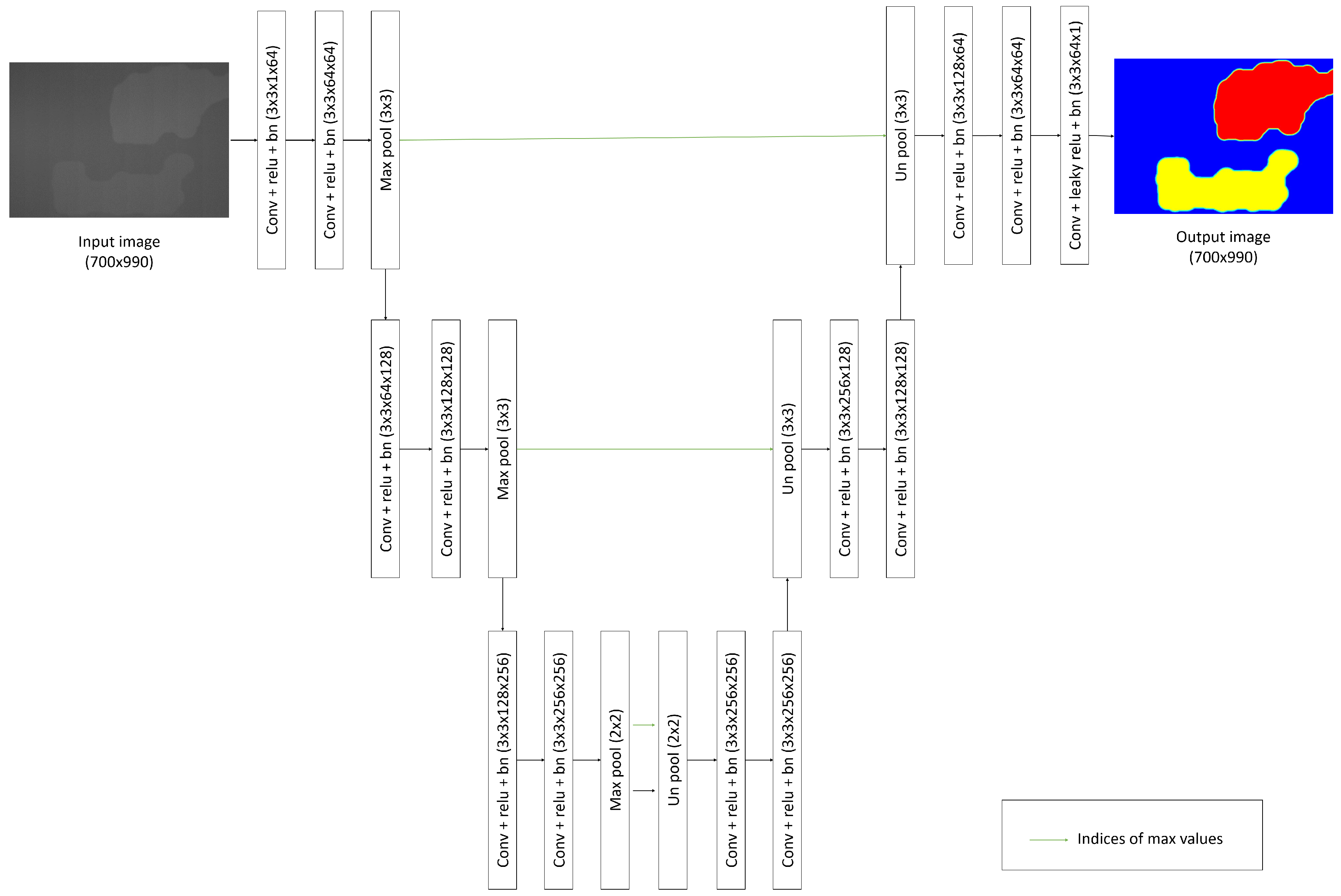
We propose a method that estimates from in (5) using an auto-encoder-based machine learning system. Figure 1 shows the architecture of the proposed auto-encoder-based machine learning system that predicts the values of the defect images. The entire system has a similar architecture to that of the auto-encoder based pixel-wise segmentation method. However, one important difference is that the final layer of the proposed system is not a softmax layer that is used for pixel-wise classification. Rather, we use a regression layer to predict the value of each pixel after removing not only the textured background but also other artifacts that are due to the imaging system. In the proposed method, the final convolutional layer in the decoder, which has only one 3 × 3 convolution acts as pixel-wise regression layer. We note that the output of the network shown in Figure 1 should be a foreground defect image (i.e., the textured-background-removed image) that has the same size as the input image.
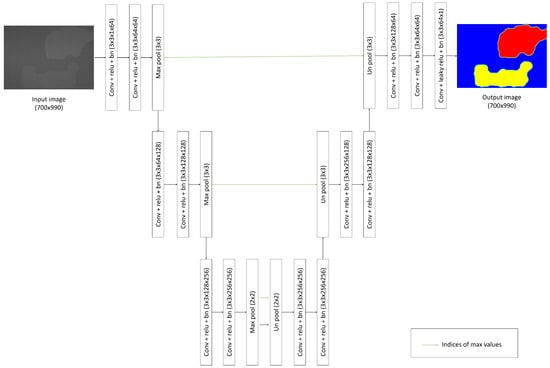
Figure 1.
Structure of the network of the proposed method.
The network consists of three encoder blocks and three decode blocks, with each encoder block consisting of two convolutional blocks and one max pooling layer, and each convolutional block consisting of one convolutional layer, a batch normalization layer and a relu layer as activation layer. Encoder blocks extract useful features, and decode blocks combine the extracted features to generate results which only have the defective parts of the image. Each decoder consist of one unpooling layer and two convolutional blocks. The size and number of kernels in the architecture are shown in Table 1.

Table 1.
The size and numbers of kernels of each layer of the proposed system.
In the last convolutional block of the decoder, we used leaky relu with slope of 0.01 for negative values as an activation function to prevent dying relu problem. In addition, the max pooling layers in the encoder blocks are connected to the unpooling layers in the corresponding decoder blocks. The connection conveys the information about the indices of max values from the max pooling layer to the unpooling layer for efficient up-sampling [14].
We design the loss function for training the network using a data fidelity term and regularization term because the use of the data fidelity term only may give rise to noisy images. First, we define the data fidelity loss function by the mean square error (MSE) between the labeled data and the predicted value according to:
where is the element at of Y that is the labeled result of the final layer of the network with the size , and is the element at of that is the calculated result of the final layer of the network with the size . The loss function calculates the mean of the square of the difference between the resulting and labeled images, and its minimization causes the result image to be close to the labeled image.
In the result image that we seek, the neighboring pixels have similar values, while the loss function that calculates only the MSE does not consider the connectivity of the pixels. This can result in scattered result images. To address this problem, we propose a loss function that calculates the MSE with total variation as the regularization term. Previously, several studies have applied the regularized loss function to machine learning systems based on the convolutional auto-encoder structure [23,24,25]. They applied a loss function with normalized cut regularization [23] and a loss function with structured edge regularization [24] to pixel-wise segmentation, and a loss function with total-variation-based regularization for pre-processing to generate a smoothed input segmentation image [25]. Using the regularization term for the loss function, these studies obtained the results reflecting the properties of the regularization term. Similar to these previous studies, we seek to obtain clustered results using a loss function with the total-variation-based regularization. The total-variation-based regularization has been used successfully for image restoration and reconstruction problems [17,18] because it can alleviate the effect of noise without the severe blurring of true edges [17].
We design the smoothness regularization function as follows:
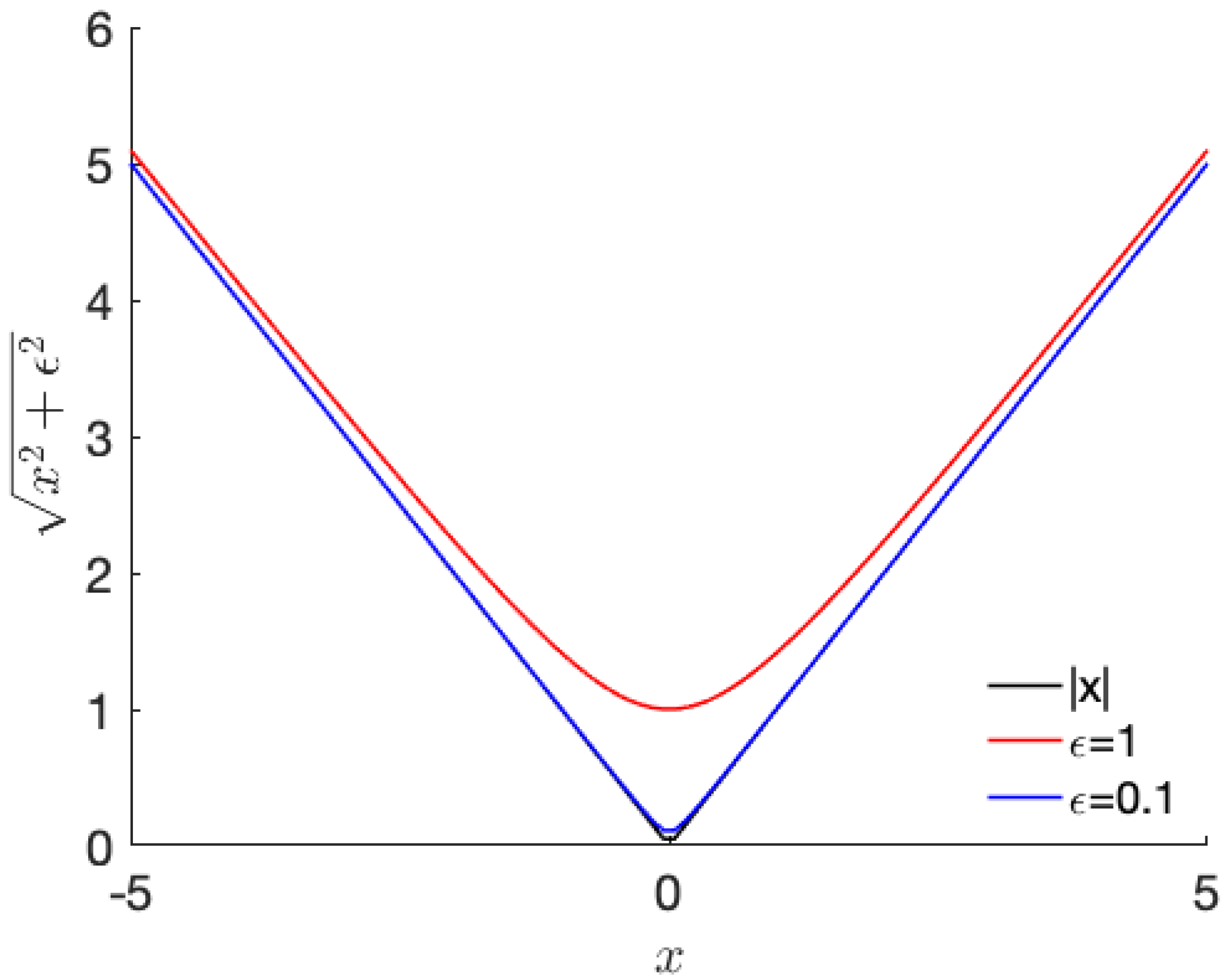
where is a design parameter, Y is the results obtained by the proposed system with the size of , and is the element of Y at . The regularization function, behaves as a 1-norm of the difference between neighbor pixels if is very small. If is large, the regularization function behaves as a 2-norm of the difference between the neighboring pixels. Therefore, it is considered that acts to control the behavior of the regularization function. Figure 2 shows the curves of for 1D case with different values of . As shown in Figure 2, the variation term in (7) approaches closer to the absolute total value with decreasing value of .
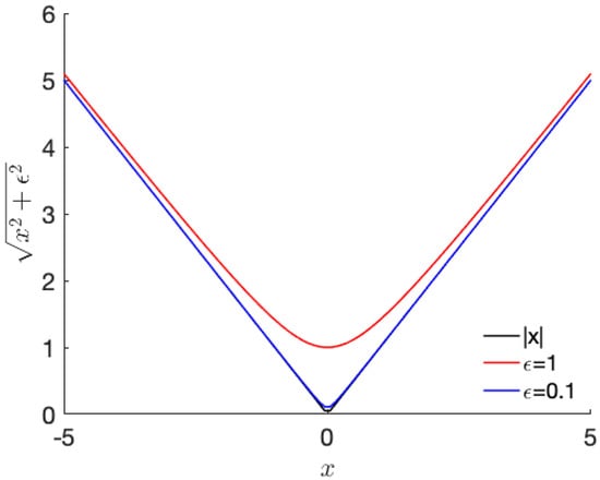
Figure 2.
Example of the change in the smoothness due to the variation in (1D).
The black line in Figure 2 indicates the total variation where is zero. By contrast, the red line shows a quadratic smoothness function near zero. Therefore, controls the behavior of the regularization function. Using the regularization function, we design an augmented total loss function as follows:
where controls the weights of the TV term that controls the smoothness. If has a large value, the result becomes smoothed, while with a small value, the result becomes less smoothed. While it may appear that the proposed method involves two hyper-parameters and , as we will show in the results section, the performance of the proposed method with and some fixed value outperforms the conventional method, implying that the tuning of hyper-parameters is not a hurdle for improving on the performance of the existing method. Rather, the introduction of the hyper-parameters is useful for improving the performance of the proposed auto-encoder-based background separation method.
4. Results
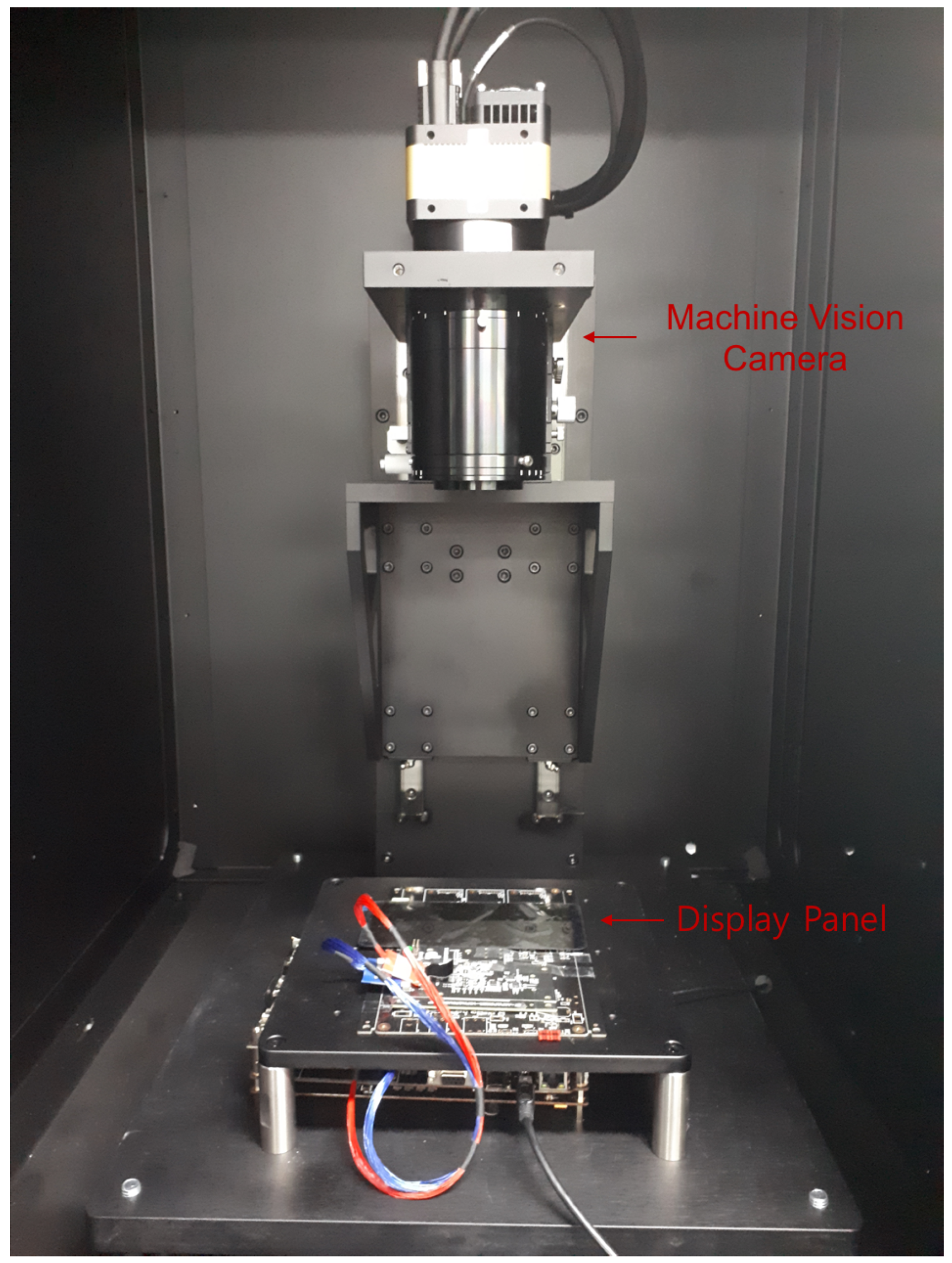
We conducted experiments to detect the defects of a 5.5 inch mobile display panels with 2880 × 1440 resolution. We acquired the images of the display panel with a machine vision camera (LPMVC-CL50M, Laon People Co., Ltd., Seongnam, Korea) in a chamber. The camera is based on 4.6 m × 4.6 m pixel size CMOS image sensor, which has monochrome pixels. Figure 3 shows the setup for our experiment.
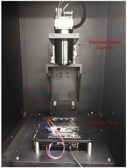
Figure 3.
Image acquisition devices.
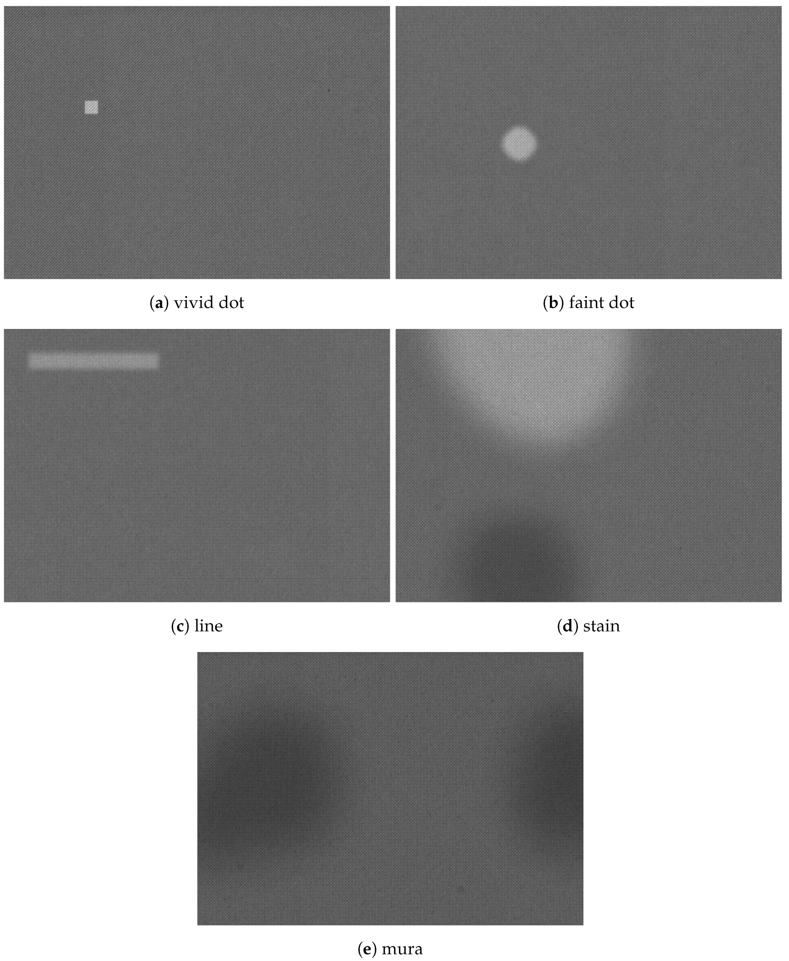
To test the performance of the proposed method through a comparison with the existing methods, we generated 5 types of defects; vivid dot, faint dot, line, stain and mura images. The vivid and faint dots have circle or square shape with relatively large and small difference from background, respectively, and the line has either horizontal or vertical linear shape. The stain defect has a faint circle type shape, and the mura defect has an irregular shape. After generating defect image, we applied Gaussian type filter for some defects to smooth the defects. We pre-determined the ranges of size, pixel intensity, length and variance of the smoothing filter. The locations, sizes and intensities of the defects are generated randomly within the pre-determined ranges. We summarize the ranges of parameters for generating defects in Table 2.
Table 2.
Ranges and settings for defects.
We displayed the generated images on the testing mobile display and acquired images using the camera. Then, we applied the proposed method to detect the generated defects with the assumption that the display is defect-free. Note that the acquired image is gray scale because the camera we used for the experiments is monochrome. The size of the acquired image was approximately 7920 × 5600. We generated a dataset that contains the fine details of the display panel by subdividing an image into regions with the size of 700 × 990. We have chosen the image size as 700 × 990 considering the limitation of GPU memories. We allowed 700 × 400 pixels overlapping to increase the number of training dataset and generated 5466 images for training. However, we did not allow overlapping for generating test dataset. The number of generated test sub-images was 6797. In summary, the entire dataset is divided into training dataset (45%) and testing dataset (55%).
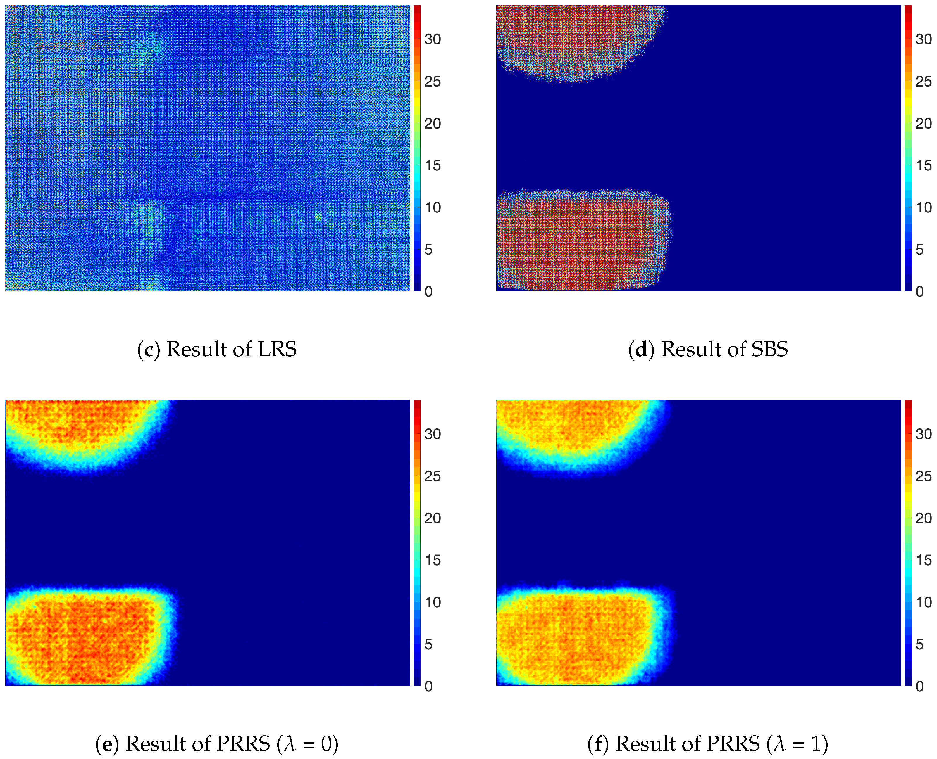
Examples of the images of the dataset are shown in Figure 4. As one can see in Figure 4, images exhibit regular patterns in the background because the pixels of the display panel are shown. We generated the ground truths for the separated foreground images manually using the information about the shape and intensity values of the patterns displayed on the device. The ground truth image has the values of the foreground only and does not contain artifacts such as the regular pattern of background, noise and non-uniform illumination.

Figure 4.
Examples of display panel images.
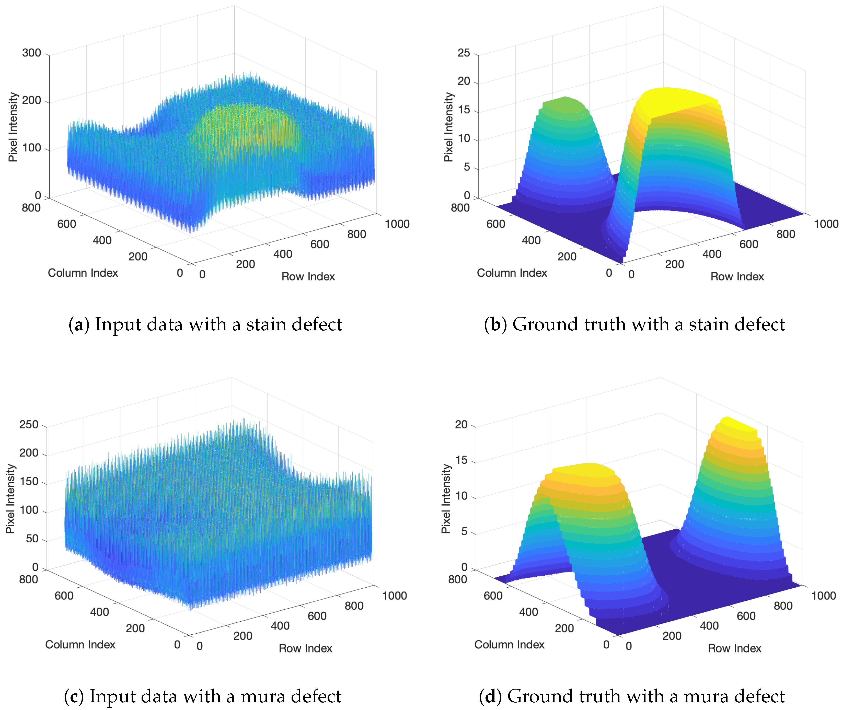
Figure 5a,b show 3D plots of the acquired image and the ground truth for each pixels with the stain and mura type defects shown in Figure 5c,d. As shown in Figure 5b,d, the ground truth is defective parts of image with no distorted components. However, in the acquired image, due to the many artifacts including non-uniform illumination, noise, and texture patterns of the background, it is difficult to separate the defects because these defects are embedded in the artifact.

Figure 5.
3D plots of the input data and result.
To detect such defects, we tested the proposed method and compared it with the SVD-based low-rank approximation method and the segmentation based method. For the segmentation based method, we used SegNet based architecture. This architecture has 3 encoder and decode blocks, and each block has 2 convolutional blocks with relu layer as activation function. In addition, the size of max pooling was for all max pooling layers in the architecture. The number of kernels of convolutional layer for each encoder block is 64, 128, 256 in order. Because SegNet architecture only divides foreground and background regions, we have implemented SegNet based segmentation and subtract the average value of background value from the segmented defect image. We refer to the low-rank approximation based method as LRS (low-rank-approximation-based separation), and the segmentation based method as SBS (segmentation based separation), and the proposed method as PRRS (pixel regression with regularization-based separation).
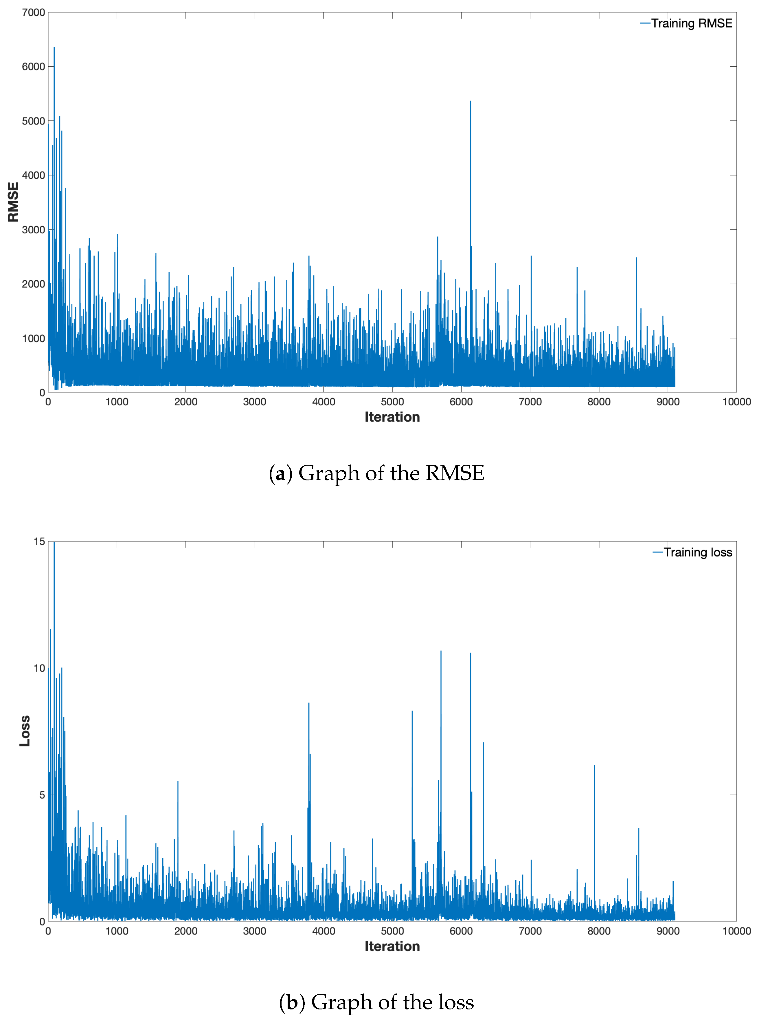
Figure 6 shows the change in loss and root-mean-square-error (RMSE) of the proposed method during training as the function of the number of iterations. In the graphs, the blue lines indicate the loss and RMSE of the training set the training loss and the validation loss, respectively. As shown in Figure 6, loss and RMSE decreased as the number of iteration increased, and gradually the variations decreased and converged.
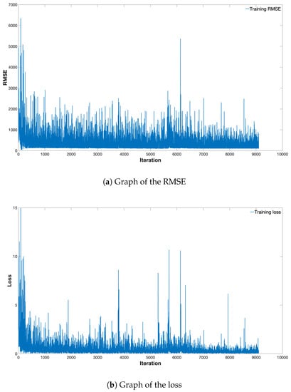
Figure 6.
Graph of the loss and RMSE during the PRRS training.
We implemented all the method for the experiments using MATLAB (2018b, MathWorks, Natick, MA, USA). We run codes for each method using a workstation with 4 TITAN Xp GPUs (NVIDIA, Santa Clara, CA, USA) and Xeon E5-2630 CPU (Intel, Santa Clara, CA, USA) with 128 Gbytes RAM. The accuracies of the result are measured by the mean absolute error (MAE) between the estimated foreground image and the ground truth, and Dice similarity coefficient [26] and intersection over union (IoU) scores [27]. For calculation of Dice and IoU, we determine regions that have positive intensity values as foreground regions.
Table 3 shows the results of LRS, SBS, PRRS with zero value of , and PRRS with the value of 1 for . We set value for PRRS method by 0.001. In the table, we showed the best result in bold. As shown in the table, PRRS showed a significantly improved performance from both the LRS and SBS in terms of MAE. In addition, PRRS with showed the best performance in terms of Dice, IoU and MAE of defective region. Note that the performance of the SBS method was better in terms of Dice and IoU than MAE. We think this is because the SBS method was able to segment defective region but failed to estimate the values of defective regions.
Table 3.
Comparative results of the proposed method with other methods.
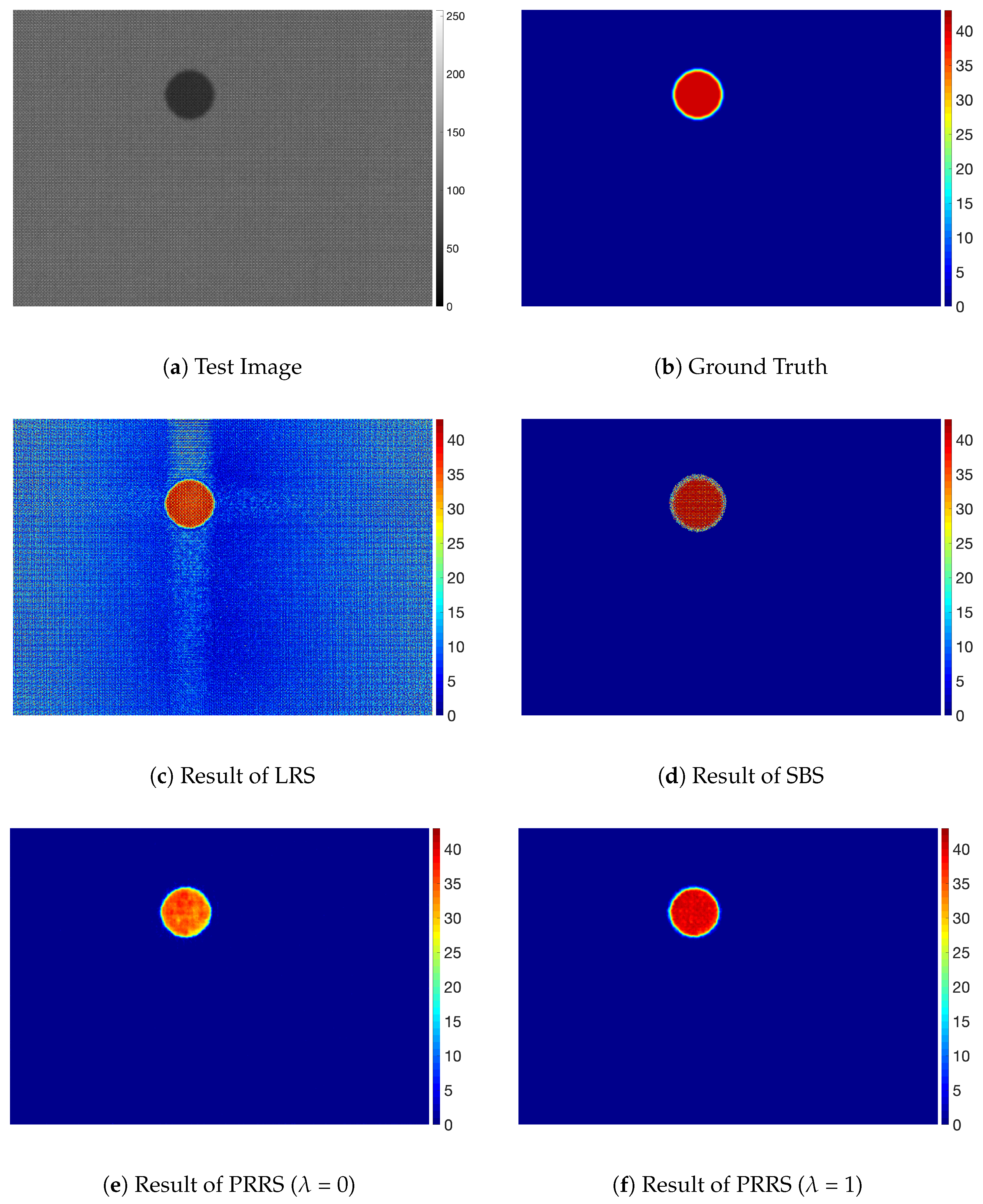
Figure 7, Figure 8 and Figure 9 show the results for the experimental dataset. Figure 7 shows the result for the faint dot type that has relatively strong edges. Although the defect is clearly visible due to the high intensity difference of the background, the LRS method was not able to remove the textured background pattern as shown in Figure 7c. This remaining background can degrade the performance of the subsequent detection method or of the quantification of defects.
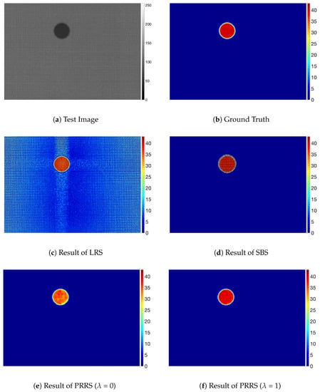
Figure 7.
Examples of display panel images with faint dot type.
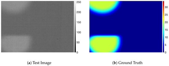
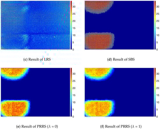
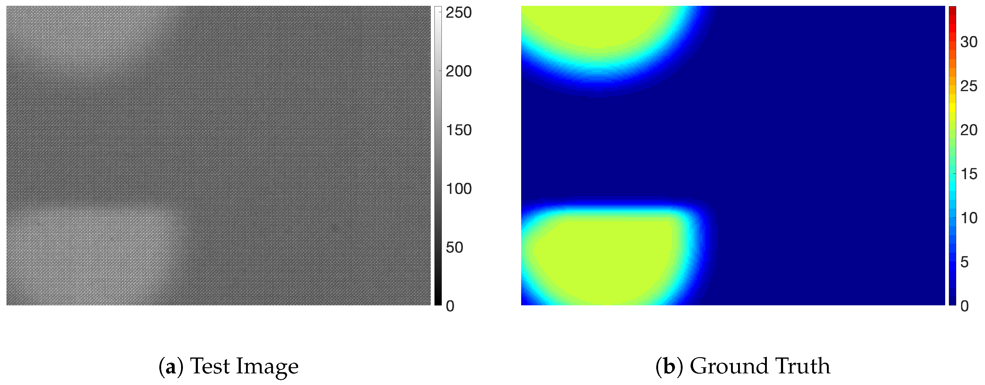
Figure 8.
Examples of display panel images with stain defects.
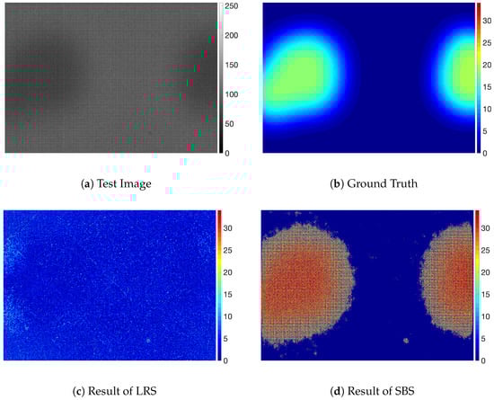
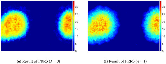
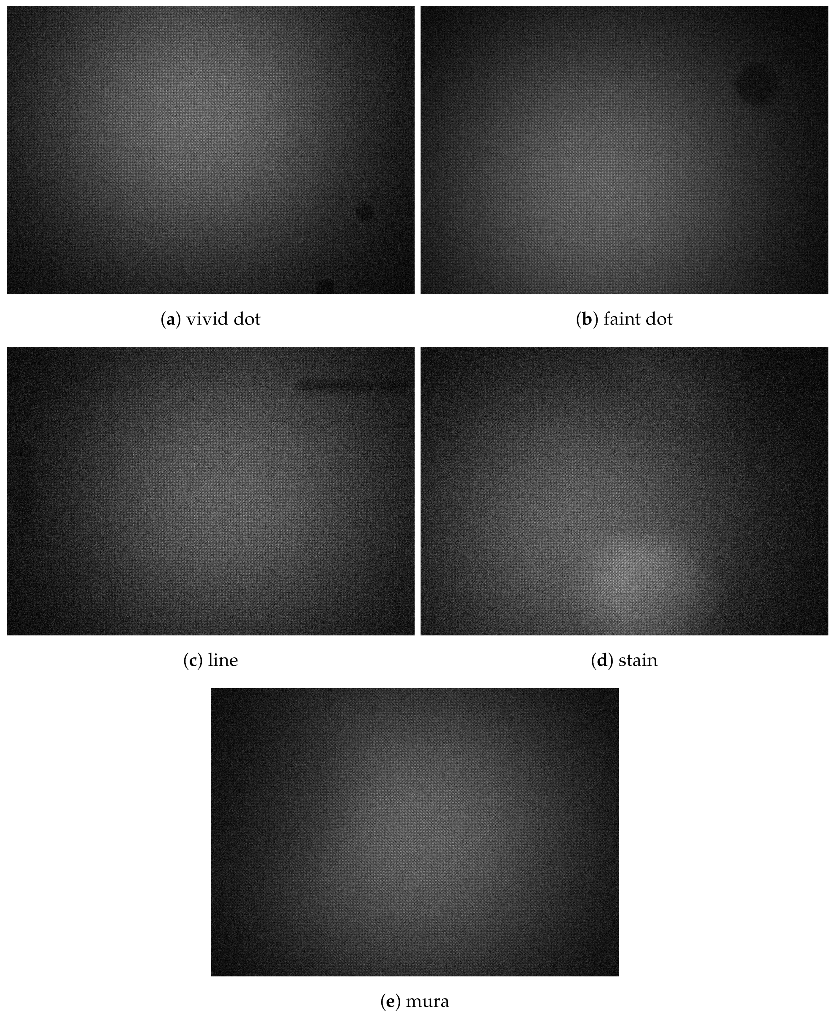
Figure 9.
Examples of display panel images with mura defects.
Figure 8 shows the result for the stain defects and Figure 9 shows the result for the mura defects. For the defects with a small intensity difference, the defects are not easily noticeable, as shown in Figure 8a and Figure 9a. The SBS method was not able to predict accurate values for the defective pixels on those defects and remove background pattern on defective pixels, as shown in Figure 8d and Figure 9d, although it was able to segment defective regions. We think this is because the SBS method is not based on a foreground estimation method but a segmentation method. On the other hand, even though the defects were not clearly visible because of the small intensity difference from the background, PRRS was able to remove the textured background and detect the defects. We have found that the texture patterns of the background are almost completely removed in the results obtained by PRRS. For all of the images, PRRS showed extremely improved results relative to LRS and SBS. In addition, PRRS with of 1 predicted more accurate values for defective pixels than PRRS with of 0. In summary, we verified that the proposed PRRS method can separate the defects from the background for various types of defects.
We have used a regularization term which has a hyper-parameter . To study the effect of the hyper-parameter, we have tested the performance of the proposed method while changing . Table 4 shows the results of the proposed method with different values of . In terms of the MAE of all region, has the best value at 1. On the other hand, in terms of the MAE of defective region, the best value of is 0.001, and from the perspective of the MAE of sound region, the best value of is 0.1. From the perspective of Dice and IoU, the best value of is 0.001. Therefore, we think that one must judiciously select the hyper-parameter considering which measure to optimize.
Table 4.
Results of the proposed method with different values of .
Table 5 summarizes the results for the proposed method with different values of . On most results of Dice and IoU, the experiment with the value of 2 for shows the best performance. However, from the perspective of MAE of defective region, the experiment with the value of 2 for shows the worst performance. Even though, it is apparent that the regularization is effective because non-zero showed better performance than zero for every case.
Table 5.
Results of the proposed method with different values of .
We also studied the effect of noise and illumination. To do that, we conducted simulation studies using a new data shown in Figure 10. We generated a new dataset adding zero-mean Gaussian noise and Gaussian shape illumination to previous dataset, as shown in Figure 10. We randomly selected variance of the Gaussian noise in the range of [0.002, 0.01]. The variance of Gaussian shape illumination was 300 pixels and the center position of Gaussian shape was determined randomly in the range of [−200, 200] from the center of an image. We refer to this dataset the shaded and noised dataset. As shown in Figure 10, it is extremely hard to distinguish defects from background.

Figure 10.
Examples of shaded and noised dataset.
Table 6 compares the results of original dataset with shaded and noised dataset. One can see that the the performance for the shaded and noised dataset is degraded from the performance using original dataset, which implies that non-uniform illumination and noise may degrade the performance of a defect separation method.
Table 6.
Results with the change of illumination and noise.
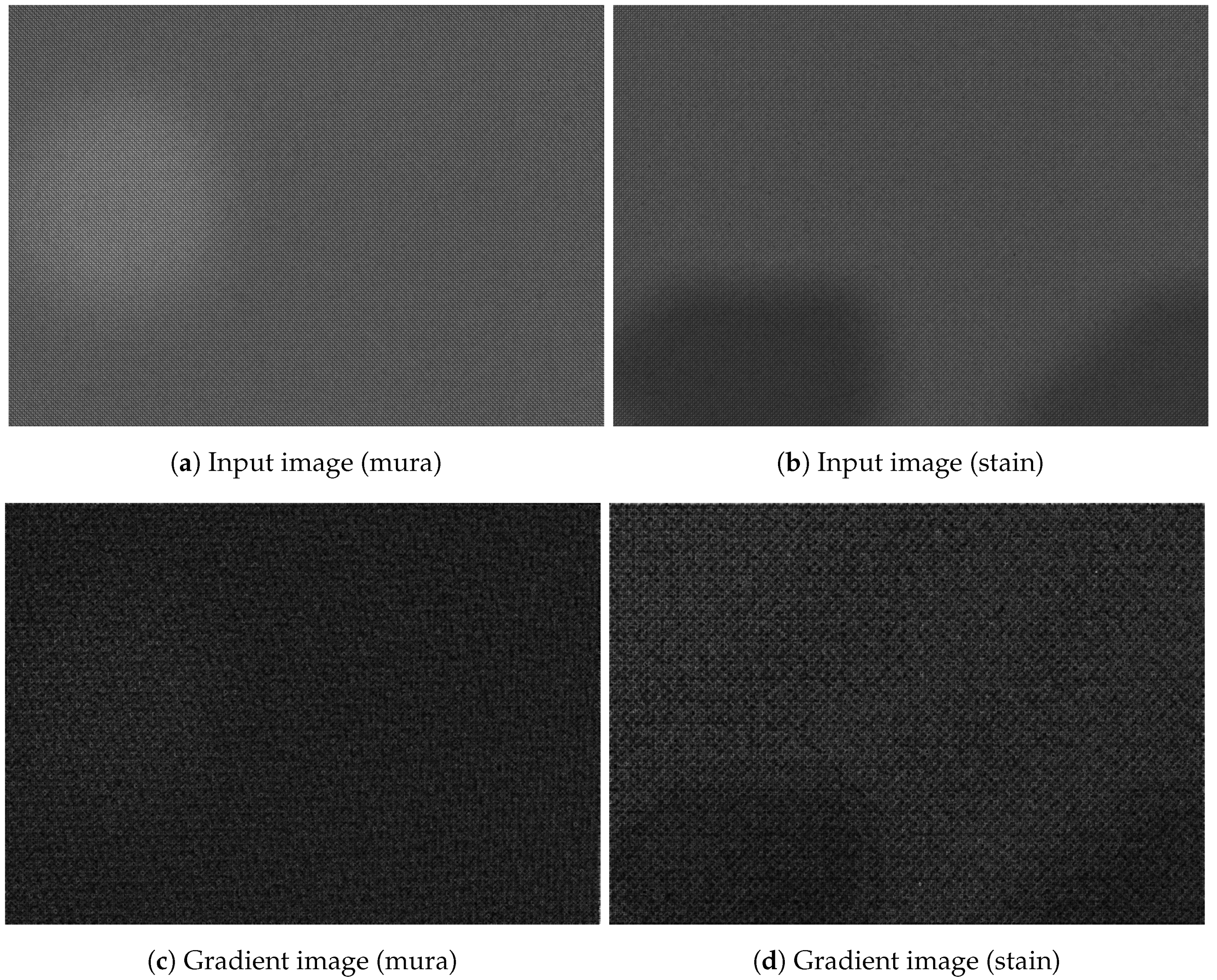
One might think that a traditional edge detection based method can separate foreground and background regions by finding edges between the two regions. For examples, one may attempt to use a gradient based method described in [28,29]. However, the edge detection based method usually fails to find boundaries due to regular texture patterns. To confirm this fact, we implemented a gradient based edge detection method which is similar to the method described in [28,29]. We first applied median filter to a display panel image and calculated magnitude of gradient for each pixel. The magnitude of gradient was calculated by summing absolute values of horizontal gradient and vertical gradient at each pixel. Figure 11 shows an example of the magnitude of gradient image. As shown in Figure 11, because there exist large gradient magnitude values inside both foreground and background regions due to texture patterns, it is extremely difficult to detect boundaries between the two regions using gradient values.
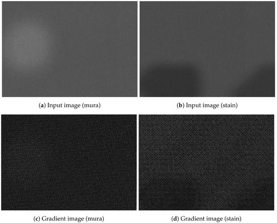
Figure 11.
Examples of result of gradient and binary images.
Inference time is one of the most important parameters in real-time systems. We measured the inference time for 100 images and averaged the testing time per one image. The testing time only includes inference time, not training time. Table 7 reports the values of the average testing time per one image for LRS and the proposed PRRS.
Table 7.
Average computation time for one image.
As shown in Table 7, LRS was faster than the proposed method. We believe this is because LRS is relatively simple and SVD can be carried out efficiently. On the other hand, the machine-learning-based PRRS requires many more computations than LRS. Nevertheless, because the computation time of PRRS is less than 320 ms, it can be applied in real-time inspection systems.
Although the inference time of the proposed method is less than 320 ms, the method needs to repeat inspection several parts of an image of mobile device. Note that the proposed method only process size image due to the limitation of computing resources.
For future works, we plan to investigate improved deep learning system to remove background patterns more perfectly. In addition, we plan investigate an automatic method to determine hyper-parameters using a method such as Bayesian optimization [30].
5. Conclusions
We proposed a novel method to separate the defects from the background using regularized auto-encoder-based regression. The conventional low-rank-approximation-based methods face difficulties in separating faint and large defects such as mura from the texture background. To address this problem, we proposed a novel method based on auto-encoder and pixel regression. During the training of the proposed system. we applied the loss function with a regularization term in order to obtain similar intensity values for the neighbor pixels in the results. In experiments using mobile display images, we verified the utility of the proposed method by a comparison to a conventional low-rank-approximation method and a segmentation-based method.
Author Contributions
H.J. conducted the experimental study and wrote the draft of the manuscript. J.K. conceived the proposed method, supervised the experiments and improved the draft.
Funding
This research was supported by Basic Science Research Program through the National Research Foundation of Korea(NRF) funded by the Ministry of Science, ICT & Future Planning (2017R1A2B4004231) and by the MOTIE (Ministry of Trade, Industry & Energy (10079560)) and Development of materials and core-technology for future display support program.
Acknowledgments
The authors are grateful to TOP engineering Co., Korea for providing us experimental devices.
Conflicts of Interest
The authors declare no conflict of interest.
References
- Baek, S.I.; Kim, W.S.; Koo, T.M.; Choi, I.; Park, K.H. Inspection of defect on LCD panel using polynomial approximation. In Proceedings of the 2004 IEEE Region 10 Conference (TENCON 2004), Chiang Mai, Thailand, 24 November 2004; pp. 235–238. [Google Scholar]
- Bi, X.; Xu, X.; Shen, J. An automatic detection method of Mura defects for liquid crystal display using real Gabor filters. In Proceedings of the 2015 8th International Congress on Image and Signal Processing (CISP), Shenyang, China, 14–16 October 2015; pp. 871–875. [Google Scholar]
- Cen, Y.G.; Zhao, R.Z.; Cen, L.H.; Cui, L.; Miao, Z.; Wei, Z. Defect inspection for TFT-LCD images based on the low-rank matrix reconstruction. Neurocomputing 2015, 149, 1206–1215. [Google Scholar] [CrossRef]
- Jamleh, H.; Li, T.Y.; Wang, S.Z.; Chen, C.W.; Kuo, C.C.; Wang, K.S.; Chen, C.C.P. 50.2: Mura detection automation in LCD panels by thresholding fused normalized gradient and second derivative responses. In SID Symposium Digest of Technical Papers; Blackwell Publishing Ltd.: Oxford, UK, 2010; Volume 41, pp. 746–749. [Google Scholar]
- Bi, X.; Zhuang, C.; Ding, H. A new mura defect inspection way for TFT-LCD using level set method. IEEE Signal Process. Lett. 2009, 16, 311–314. [Google Scholar]
- Chen, L.C.; Kuo, C.C. Automatic TFT-LCD mura defect inspection using discrete cosine transform-based background filtering and ‘just noticeable difference’quantification strategies. Meas. Sci. Technol. 2007, 19, 015507. [Google Scholar] [CrossRef]
- Wang, Z.; Gao, J.; Jian, C.; Cen, Y.; Chen, X. OLED Defect Inspection System Development through Independent Component Analysis. TELKOMNIKA Indones. J. Electr. Eng. 2012, 10, 2309–2319. [Google Scholar] [CrossRef]
- Lu, C.J.; Tsai, D.M. Automatic defect inspection for LCDs using singular value decomposition. Int. J. Adv. Manuf. Technol. 2004, 25, 53–61. [Google Scholar] [CrossRef]
- Lu, C.J.; Tsai, D.M. Defect inspection of patterned thin film transistor-liquid crystal display panels using a fast sub-image-based singular value decomposition. Int. J. Prod. Res. 2007, 42, 4331–4351. [Google Scholar] [CrossRef]
- Perng, D.B.; Chen, S.H. Directional textures auto-inspection using discrete cosine transform. Int. J. Prod. Res. 2011, 49, 7171–7187. [Google Scholar] [CrossRef]
- Chen, S.H.; Perng, D.B. Directional textures auto-inspection using principal component analysis. Int. J. Adv. Manuf. Technol. 2011, 55, 1099–1110. [Google Scholar] [CrossRef]
- Gan, Y.; Zhao, Q. An effective defect inspection method for LCD using active contour model. IEEE Trans. Instrum. Meas. 2013, 62, 2438–2445. [Google Scholar] [CrossRef]
- Tseng, D.C.; Lee, Y.C.; Shie, C.E. LCD mura detection with multi-image accumulation and multi-resolution background subtraction. Int. J. Innov. Comput. Inf. Control 2012, 8, 4837–4850. [Google Scholar]
- Badrinarayanan, V.; Kendall, A.; Cipolla, R. SegNet: A Deep Convolutional Encoder-Decoder Architecture for Image Segmentation. IEEE Trans. Pattern Anal. Mach. Intell. 2017, 39, 2481–2495. [Google Scholar] [CrossRef] [PubMed]
- Ronneberger, O.; Fischer, P.; Brox, T. U-net: Convolutional networks for biomedical image segmentation. In Proceedings of the International Conference on Medical Image Computing and Computer-Assisted Intervention, Munich, Germany, 5–9 October 2015; pp. 234–241. [Google Scholar]
- Kumar, P.; Nagar, P.; Arora, C.; Gupta, A. U-Segnet: Fully Convolutional Neural Network Based Automated Brain Tissue Segmentation Tool. In Proceedings of the 2018 25th IEEE International Conference on Image Processing (ICIP), Athens, Greece, 7–10 October 2018; pp. 3503–3507. [Google Scholar]
- Chen, Q.; Montesinos, P.; Sen Sun, Q.; Heng, P.A.; Xia, D.S. Adaptive total variation denoising based on difference curvature. Image Vis. Comput. 2010, 28, 298–306. [Google Scholar] [CrossRef]
- Block, K.T.; Uecker, M.; Frahm, J. Undersampled radial MRI with multiple coils. Iterative image reconstruction using a total variation constraint. Magn. Reson. Med. 2007, 57, 1086–1098. [Google Scholar] [CrossRef] [PubMed]
- Anderson, D.; Sweeney, J.; Williams, T. Statistics for Business and Economics. South-Western; Thomson Learning Publishing Company: Cincinnati, OH, USA, 2002. [Google Scholar]
- Jenkins, M.D.; Carr, T.A.; Iglesias, M.I.; Buggy, T.; Morison, G. A Deep Convolutional Neural Network for Semantic Pixel-Wise Segmentation of Road and Pavement Surface Cracks. In Proceedings of the 2018 26th European Signal Processing Conference (EUSIPCO), Rome, Italy, 3–7 September 2018; pp. 2120–2124. [Google Scholar]
- Naresh, Y.G.; Little, S.; O’Connor, N.E. A Residual Encoder-Decoder Network for Semantic Segmentation in Autonomous Driving Scenarios. In Proceedings of the 2018 26th European Signal Processing Conference (EUSIPCO), Rome, Italy, 3–7 September 2018. [Google Scholar]
- Kendall, A.; Badrinarayanan, V.; Cipolla, R. Bayesian segnet: Model uncertainty in deep convolutional encoder-decoder architectures for scene understanding. arXiv 2015, arXiv:1511.02680. [Google Scholar]
- Tang, M.; Djelouah, A.; Perazzi, F.; Boykov, Y.; Schroers, C. Normalized cut loss for weakly-supervised CNN segmentation. In Proceedings of the IEEE Conference on Computer Vision and Pattern Recognition, Salt Lake City, UT, USA, 18–22 June 2018; pp. 1818–1827. [Google Scholar]
- Cheng, D.; Meng, G.; Cheng, G.; Pan, C. SeNet: Structured edge network for sea–land segmentation. IEEE Geosci. Remote Sens. Lett. 2017, 14, 247–251. [Google Scholar] [CrossRef]
- Wang, C.; Yang, B.; Liao, Y. Unsupervised image segmentation using convolutional autoencoder with total variation regularization as preprocessing. In Proceedings of the 2017 IEEE International Conference on Acoustics, Speech and Signal Processing (ICASSP), New Orleans, LA, USA, 5–9 March 2017; pp. 1877–1881. [Google Scholar]
- Dice, L.R. Measures of the amount of ecologic association between species. Ecology 1945, 26, 297–302. [Google Scholar] [CrossRef]
- Csurka, G.; Larlus, D.; Perronnin, F.; Meylan, F. What is a good evaluation measure for semantic segmentation? BMVC 2013, 27, 2013. [Google Scholar]
- Dorafshan, S.; Thomas, R.J.; Maguire, M. Comparison of deep convolutional neural networks and edge detectors for image-based crack detection in concrete. Constr. Build. Mater. 2018, 186, 1031–1045. [Google Scholar] [CrossRef]
- Dorafshan, S.; Maguire, M.; Qi, X. Automatic Surface Crack Detection in Concrete Structures Using Otsu Thresholding and Morphological Operations; Technical Report 1234; Civil and Environmental Engineering Faculty Publications, Utah State University: Logan, UT, USA, 2016. [Google Scholar]
- Shahriari, B.; Swersky, K.; Wang, Z.; Adams, R.P.; De Freitas, N. Taking the human out of the loop: A review of bayesian optimization. Proc. IEEE 2016, 104, 148–175. [Google Scholar] [CrossRef]


© 2019 by the authors. Licensee MDPI, Basel, Switzerland. This article is an open access article distributed under the terms and conditions of the Creative Commons Attribution (CC BY) license (http://creativecommons.org/licenses/by/4.0/).