An Efficient Hardware Accelerator for the MUSIC Algorithm

Abstract

As a classical DOA (direction of arrival) estimation algorithm, the multiple signal classification (MUSIC) algorithm can estimate the direction of signal incidence. A major bottleneck in the application of this algorithm is the large computation amount, so accelerating the algorithm to meet the requirements of high real-time and high precision is the focus. In this paper, we design an efficient and reconfigurable accelerator to implement the MUSIC algorithm. Initially, we propose a hardware-friendly MUSIC algorithm without the eigenstructure decomposition of the covariance matrix, which is time consuming and accounts for about 60% of the whole computation. Furthermore, to reduce the computation of the covariance matrix, this paper utilizes the conjugate symmetry property of it and the way of iterative storage, which can also lessen memory access time. Finally, we adopt the stepwise search method to realize the spectral peak search, which can meet the requirements of 1° and 0.1° precision. The accelerator can operate at a maximum frequency of 1 GHz with a 4,765,475.4 μm² area, and the power dissipation is 238.27 mW after the gate-level synthesis under the TSMC 40-nm CMOS technology with the Synopsys Design Compiler. Our implementation can accelerate the algorithm to meet the high real-time and high precision requirements in applications. Assuming that the case is an eight-element uniform linear array, a single signal source, and 128 snapshots, the computation times of the algorithm in our architecture are 2.8 μs and 22.7 μs for covariance matrix estimation and spectral peak search, respectively.

1. Introduction

The calculation of the direction of a signal source is a common issue in the fields of civilian and military communication; one outstanding application of such techniques in mobile communications is wireless location services in cellular systems such as GSM (Global System for Mobile Communications), DS-CDMA (direct sequence-code division multiple access) systems, etc. The MUSIC (multiple signal classification) algorithm is the most classic among those DOA estimation methods based on spatial spectrum estimation [1,2], which was first proposed by R.O. Schmidt, and it created a new era of spatial spectrum estimation algorithm research. It achieves high precision and high resolution in the use of non-coherence signal source distinguishing and sensing and is widely cited and modified in areas such as sensing, communication, radar, and so on. However, its need for estimation and eigenstructure decomposition of the covariance matrix leads to large data storage and computing, which makes the real-time implementation difficult and is not hardware friendly for hardware implementation. Therefore, we want to design an efficient and reconfigurable accelerator to implement the MUSIC algorithm to satisfy the requirements of high real-time and high precision in the above applications. In order to achieve this goal, we study it from the perspective of algorithm and hardware implementation, respectively.

From the algorithmic perspective, in order to reduce the computation of the MUSIC algorithm, many papers have been committed to improving the MUSIC algorithm. The root-MUSIC algorithm [3] utilizes the rooting process instead of spectral search to greatly reduce the computational cost. Of course, some improved root-MUSIC algorithms [4,5] have since emerged; however, essentially, nothing has changed, and they still have to calculate the eigenvalue decomposition. The MUSIC algorithm based on spatial smoothing technology (SST-MUSIC) in [6,7,8] can also correctly distinguish coherent signals. It sacrifices effective array elements to ensure the full rank of the covariance matrix and then uses the classical MUSIC algorithm to estimate spectrum to obtain the DOA (direction of arrival) of relevant signals. Besides, the IMUSIC (improved MUSIC) algorithm in [9] and the MMUSIC (modified MUSIC) algorithm in [10] can not only recognize coherent signals, but can also accurately identify signals with small SNR (signal to noise ratio) and small angle interval. The work in [9] corrected the MUSIC algorithm by preprocessing coherent signals from the perspective of noise subspace so that the corrected noise subspace is fully orthogonal to the direction matrix. The work in [10] made full use of the received data information and extra calculation of the cross-covariance matrix to improve the performance of the algorithm. Although these improved algorithms more or less change the computation or performance of the MUSIC algorithm, they all have one common feature: calculating EVD (eigenvalue decomposition). As we all know, EVD consumes much computing time and takes up about 60% of the total MUSIC calculation [11]. Improving or removing EVD will play an important role in reducing the calculation time of the MUSIC algorithm.

From the hardware perspective, with the requirements of high performance and flexibility in embedded design, various hardware accelerated processors come into being, such as DSP, FPGA, and ASIC. FPGA can achieve great performance, but lacks certain flexibility. DSP can accomplish the algorithm by software programming, which is more flexible than FPGA, but the features of DSP are a limit to using it in real-time applications. Among those processors, reconfigurable computing [12,13,14] is becoming more promising because reconfigurable architectures are flexible, scalable, and provide reasonable computing capability. Although there are many hardware accelerators to implement the MUSIC algorithm [15,16,17], few reconfigurable processors are found. From what has been discussed above, the reconfigurable architecture is a balanced solution to implement the MUSIC algorithm.

Therefore, this paper designs an efficient and reconfigurable accelerator to implement the MUSIC algorithm. In order to reduce the computational complexity of the MUSIC algorithm, this paper firstly optimizes the MUSIC algorithm and proposes a hardware-friendly MUSIC algorithm (HFMA), in which the signal subspace is achieved by the sub-matrix of the array covariance matrix without eigenstructure decomposition. Secondly, despite the covariance matrix being often obtained by a matrix multiplication [18,19], the calculation amount can be reduced by using its conjugate symmetry property (CSP), and the data exchange time from on-chip to off-chip can be decreased by way of iterative storage. Finally, this paper adopts the stepwise search method to improve the precision of spectral peak search, and it is compatible with both the 1° and 0.1° precision requirements. According to the above scheme, the total time of the HFMA implemented in the accelerator is 25.5 μs, which can meet the real-time demand of the MUSIC algorithm application. The accelerator can operate at a maximum frequency of 1 GHz with a 4,765,475.4 μm² area, and the power dissipation is 238.27 mW after the gate-level synthesis under the TSMC 40-nm CMOS technology with the Synopsys Design Compiler.

On the whole, this paper makes the following contributions:

• Showing the details of an HFMA without the EVD of the covariance matrix, which is time consuming with high computational cost and complex for hardware implementations. The HFMA has far fewer computations compared with the classical MUSIC algorithm at the expense of a small performance decrease, but it proves to be efficient through theoretical analysis, simulation, and hardware implementation.
• Designing an efficient hardware accelerator to implement the HFMA. Based on a processing element (PE) array consisting of different functional units, multiple sub-algorithms can be implemented through the reconfigurable controller. Combining the sub-algorithms in the accelerator, we can implement the HFMA under the reconfigurable architecture.
• Using the CSP of the covariance matrix and the way of iterative storage to compute the correlation matrix estimation, which can reduce the computation and memory access time. It is a sub-algorithm in the accelerator and can support a matrix with arbitrary columns. Especially, compared with TMS320C6672 [20,21], which has similar computing resources, the computation period of the covariance matrix can be shortened by 3.5–5.8× after the resource normalization.
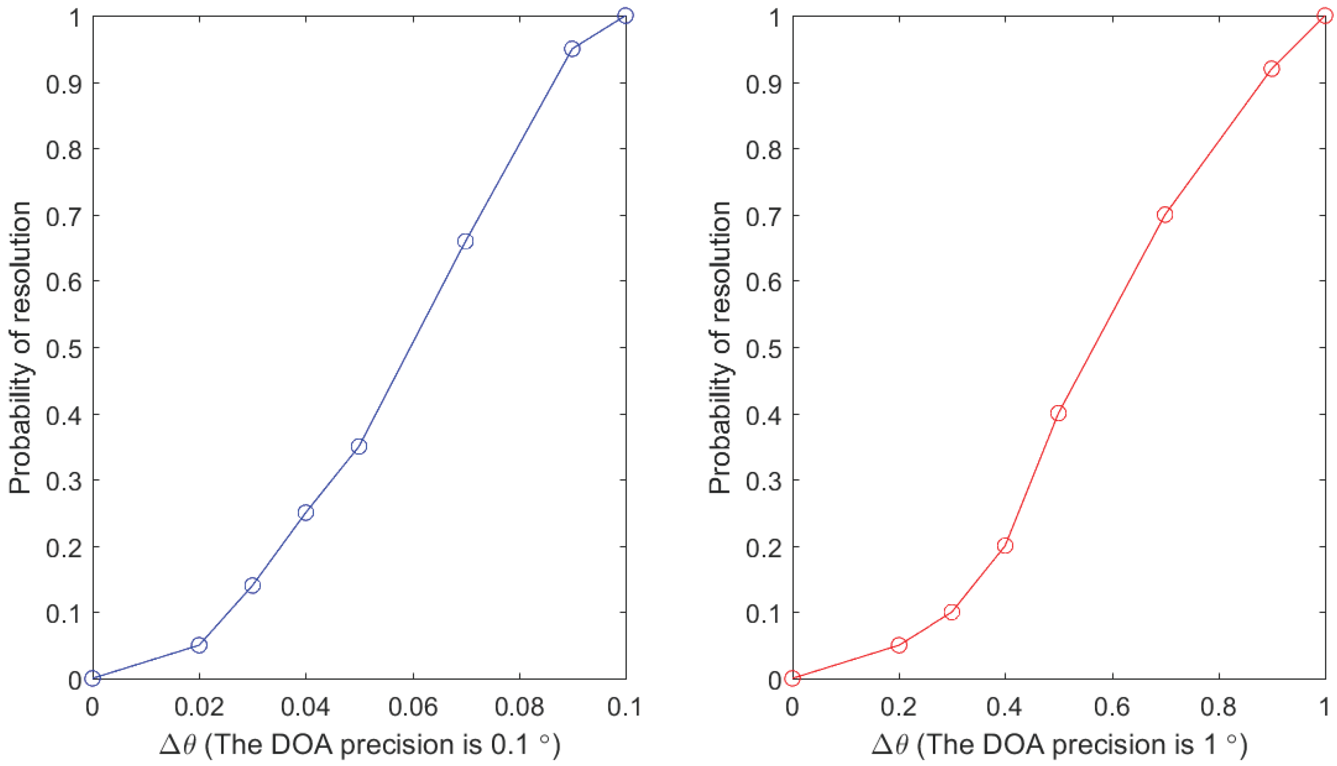
• Utilizing the reconfigurable method to decompose the spectral peak search into several sub-algorithms and also using a stepwise search method to implement the spectral peak search. When high precision is required, the larger step size is first set for the rough search in the whole range, and then, the search precision is taken as the second step size for the precise search near the first search result. The spectrum peak search in this paper is compatible with both the 1° and 0.1° accuracy requirements.

The notations employed in this paper are listed in

Table 1. Notations in this paper.

Notation	Definition
Q	the number of input signals
$S_q\left(t\right)$	the qth narrowband non-coherent signal
M	the number of the array element
d	the distance between two contiguous array elements
$\lambda$	the wavelength of the source signal
${\alpha }_q$	the angle between the qth incident wave and the array
$x_m\left(t\right)$	the received signal of the mth array element
$n_m\left(t\right)$	the zero-mean white noise of the mth array element
$X\left(t\right)$	the formed matrix
$c\left({\alpha }_q\right)$	the directional vector of the array
C	the array manifold
$S\left(t\right)$	the incident signal vector
$N\left(t\right)$	the incident noise vector
$x\left(k\right)$	the kth array input sampling
K	the snapshot number
R	the estimate of the array covariance matrix
${\delta }^2$	the power of noise
$I_M$	the Mth order unit matrix
${\alpha }_q$	the estimate of the DOA of the qth incident signal
$v_m$	the mth normalized orthogonal eigenvector
$V_s$	the subspace of the estimated signal
$V_n$	the subspace of the estimated noise
$Q_{MUSIC}$	the MUSIC spatial spectrum
$A,B$	the row and column number of the matrix, respectively
D	the zones of the partitioned banks
$BS$	the depth of each bank
P	the number of banks to store the lower triangular matrix
E	the number of banks to store the source data
$addrX$	the number of data
$COL$	the column number of the matrix
$matrix\_row$	the row of the data in the matrix
$matrix\_column$	the column of the data in the matrix
$bank\_num$	the number of the data in the bank
$bank\_addr$	the address of the data in the bank
${\widehat{Q}}_{last}$	the value of spatial spectral function after deformation
$B{P}_r$	the balanced performance ratio
$C{P}_{ref},C{P}_{pro}$	the computation periods of the reference and this paper, respectively
$Slic{e}_{ref},Slic{e}_{pro}$	the slices of the reference and this paper, respectively
$C{P}_r$	the computation period ratio
$Slic{e}_r$	the slice ratio

for clearer representation.

The organization of the paper in the rest of the sections is as follows: Section 2 introduces the classical MUSIC algorithm and the optimized HFMA. Section 3 details the architecture of the efficient and reconfigurable accelerator and presents the design of the covariance matrix and the spectral peak search. The experimental results and analysis are given in Section 4. Finally, a conclusion of the paper is presented.

2. Backgrounds

Generally, the MUSIC algorithm consists of three parts: solving the covariance matrix based on the input, calculating its eigenvalue and eigenvector based on the covariance matrix, and conducting spectrum peak search based on the eigenvalue and eigenvector. In order to reduce the computation amount of the MUSIC algorithm and improve the speed of hardware implementation, we firstly analyze the characteristics of the MUSIC algorithm and then propose the HFMA. Therefore, this section firstly sets up a signal model and describes the classical MUSIC algorithm. Then, the HFMA is proposed, which can avoid the most time-consuming eigenvalue decomposition.

2.1. The Array Model and the MUSIC Algorithm

Provided Q narrowband non-coherent signals $S_q\left(t\right)$, ($q=1,2,\dots ,Q$) from the distant field reach the uniform linear array (ULA), which is formed with M array elements. d represents the distance between two contiguous array elements, and $\lambda$ is the wavelength of the source signal. The signal is received from the source with $X\left(t\right)$ and $S\left(t\right)$, where ${\alpha }_q$ is the angle between the direction of the qth incident wave and the array. If the first array element acts as a reference array element, the received signal of the mth array element is:

$$x_m\left(t\right)=\sum _{q=1}^Q{S}_q\left(t\right)e^{j2\pi (m-1)dcos{\alpha }_q/\lambda }+n_m\left(t\right),$$

(1)

where $m=1,2,\dots ,M$, $n_m\left(t\right)$ is the zero-mean white noise of the mth array element and independent of each array element.

Assuming that $X\left(t\right)={[x_1\left(t\right),x_2\left(t\right),\dots ,x_M\left(t\right)]}^T$, the directional vector of the array $c\left({\alpha }_q\right)={[1,e^{\frac{j2\pi dcos{\alpha }_q}{\lambda }},\dots ,e^{\frac{j2\pi (M-1)dcos{\alpha }_q}{\lambda }}]}^T$, the array manifold $C={[c\left({\alpha }_1\right),\dots ,c\left({\alpha }_q\right)]}^T$, the incident signal vector $S\left(t\right)={[s_1\left(t\right),\dots ,s_Q\left(t\right)]}^T$, and $N\left(t\right)={[n_1\left(t\right),\dots ,n_M\left(t\right)]}^T$, we can calculate the array input sampling:

$$x\left(k\right)=C\times s\left(k\right)+n\left(k\right),$$

(2)

where $k=1,2,\dots ,K$, $x\left(k\right)$, $s\left(k\right)$, $n\left(k\right)$ are the kth samples, respectively, and K is the snapshot number. Thus, the estimate of the array covariance matrix in actual applications and simulations is shown by:

$$R=C\times E[S\left(t\right)S^H\left(t\right)]\times C^H+{\delta }^2{I}_M,$$

(3)

where $C\times E[S\left(t\right)S^H\left(t\right)]\times C^H$ is the signal covariance matrix and $E[S\left(t\right)S^H\left(t\right)]$ is the correlation matrix of the signal complex envelop; ${\delta }^2$ is the power of noise, and $I_M$ is the Mth order unit matrix. Therefore, ${\delta }^2{I}_M$ is the noise covariance matrix, that is $E[N\left(t\right)N^H\left(t\right)]$. The target of DOA estimate is to get ${\alpha }_q$ or C from Equation (3).

When $Q<M$, R has M eigenvalues ${\lambda }_1\ge {\lambda }_2\ge \dots \ge {\lambda }_Q\ge {\lambda }_{Q+1}={\lambda }_{Q+2}=\dots ={\lambda }_M={\delta }^2$ and corresponding M normalized orthogonal eigenvectors $v_m$. ${\lambda }_1,\dots ,{\lambda }_Q$ are the eigenvalues corresponding to the signal, and ${\lambda }_{Q+1},\dots ,{\lambda }_M$ are the eigenvalues corresponding to the noise.

Define $V_s=[v_1,v_2,\dots ,v_Q]$, $V_n=[v_{Q+1},v_{Q+2},\dots ,v_M]$, then the column vector of $V_s$ and $V_n$ is the subspace of the estimated signal and noise, respectively. We will get:

$$Q_{MUSIC}=c^H({\alpha }_q)V_s{V}_s^{H}c({\alpha }_q)=\frac{1}{c^H({\alpha }_q)V_n{V}_n^{H}c({\alpha }_q)}$$

(4)

and the result ${\alpha }_q$ is the estimate of the DOA of the qth incident signal.

2.2. The Hardware-Friendly MUSIC Algorithm

Based on the above array model and the classical MUSIC algorithm, we can make attempts to estimate the signal subspace by a submatrix $R_{sub}$ instead of doing the eigenstructure decomposition of R.

Define $X_{sub}\left(m\right)={[x_1\left(t\right),x_2\left(t\right),\dots ,x_m\left(t\right)]}^T$, $N_{sub}\left(m\right)={[n_1\left(t\right),n_2\left(t\right),\dots ,n_m\left(t\right)]}^T$ and matrix $C_{sub}\left(m\right)$ formed by first m rows in C; its columns are signal directional vectors $c_{sub}(m,{\alpha }_q)$ to the $m^{\mathrm{th}}$ order sub-matrix of $c\left({\alpha }_q\right)$. Let ${X_{sub}}^{\prime }\left(Q\right)={[x_{Q+1}\left(t\right),x_{Q+2}\left(t\right),\dots ,x_M\left(t\right)]}^T$, ${N_{sub}}^{\prime }\left(Q\right)={[n_{Q+1}\left(t\right),n_{Q+2}\left(t\right),\dots ,n_M\left(t\right)]}^T$; thus:

$$X\left(t\right)=\left[\begin{array}{c}{X}_{sub}\left(Q\right)\\ {X_{sub}}^{\prime }\left(Q\right)\end{array}\right],N\left(t\right)=\left[\begin{array}{c}{N}_{sub}\left(Q\right)\\ {N_{sub}}^{\prime }\left(Q\right)\end{array}\right],C\left(t\right)=\left[\begin{array}{c}{C}_{sub}\left(Q\right)\\ {C_{sub}}^{\prime }\left(Q\right)\end{array}\right].$$

(5)

$R_{sub}$ is formed by the (Q + 1 )th to Mth rows, first to the Qth columns of R, namely:

$$R_{sub}=E[{X_{sub}}^{\prime }\left(Q\right)X_{sub}{\left(Q\right)}^H]=\frac{{\sum }_{k=1}^K{x_{sub}}^{\prime }(Q,k){x_{sub}}^H(Q,k)}{K}.$$

(6)

Then, we can reason it out that:

$$\begin{array}{c}\hfill \begin{array}{cc}\hfill {C_{sub}}^{\prime }\left(Q\right)& =\left[\begin{array}{ccc}{e}^{\frac{j2\pi dQcos{\alpha }_1}{\lambda }}& \cdots & e^{\frac{j2\pi dQcos{\alpha }_Q}{\lambda }}\\ ⋮& \ddots & ⋮\\ e^{\frac{j2\pi d(M-1)cos{\alpha }_1}{\lambda }}& \cdots & e^{\frac{j2\pi d(M-1)cos{\alpha }_Q}{\lambda }}\end{array}\right]\hfill \\ & =\left[\begin{array}{ccc}1& \cdots & 1\\ ⋮& \ddots & ⋮\\ e^{\frac{j2\pi d(M-Q-1)cos{\alpha }_1}{\lambda }}& \cdots & e^{\frac{j2\pi d(M-Q-1)cos{\alpha }_Q}{\lambda }}\end{array}\right]·diag[e^{\frac{j2\pi dQcos{\alpha }_1}{\lambda }},\dots ,e^{\frac{j2\pi dQcos{\alpha }_Q}{\lambda }}]\hfill \\ & =C_{sub}(M-Q){\wedge }^Q,\hfill \end{array}\end{array}$$

(7)

where $\wedge =diag[e^{\frac{j2\pi dcos{\alpha }_1}{\lambda }},\dots ,e^{\frac{j2\pi dcos{\alpha }_Q}{\lambda }}]$. Further analysis shows that:

$$\begin{array}{c}\hfill \begin{array}{cc}\hfill R_{sub}& =E\{[C_{sub}(M-Q){\wedge }^{Q}S\left(t\right)+{N_{sub}}^{\prime }\left(Q\right)]{[C_{sub}\left(Q\right)S\left(t\right)+N_{sub}\left(Q\right)]}^H\}\hfill \\ & =C_{sub}(M-Q){\wedge }^{Q}E[S\left(t\right)S^H\left(t\right)]C_{sub}^H\left(Q\right).\hfill \end{array}\end{array}$$

(8)

From Equation (8), we know that $R_{sub}$ can be represented by $C_{sub}(M-Q)$ linearly. If $Q<(M-Q)$, when Q signals arrive from different directions, the rank of $C_{sub}^H\left(Q\right)$ is $\Gamma \left(C_{sub}^H\left(Q\right)\right)$ and $\Gamma \left({\Lambda }^Q\right)=\Gamma \left(E\left[S\left(t\right)S^H\left(t\right)\right]\right)=Q$, so the column vector group of $R_{sub}$ and $C_{sub}(M-Q)$ forms the same sub-space, which is the signal sub-space formed by signal vectors of $(M-Q)$ dimensions.

In order to calculate the HFMA, we firstly calculate the $(M-Q)\times Q$ order sub-matrix $R_{sub}$ as Equation (8). Next, we perform standardization and orthogonalization on the columns of $R_{sub}$ and denote the resulting matrix formed by column vectors as $V_{sub}$. Finally, we make estimation on ${\alpha }_q$ by spectral peak searching on the following function. That is:

$$\widehat{Q}({\alpha }_q)=c_{sub}{(M-Q,{\alpha }_q)}^H{V}_{sub}{V}_{sub}^H{c}_{sub}(M-Q,{\alpha }_q).$$

(9)

The HFMA needs neither eigenstructure decomposition, nor estimation of the whole covariance matrix, which has far less computation than the classical MUSIC algorithm. Although the performance decreases compared with the MUSIC algorithm without dimension-reduction, when Q is far less than M, the performance decrease is acceptable [22], which matches the theoretical analysis.

3. Implementation of the HFMA

In this section, we design an efficient and reconfigurable accelerator to implement the HFMA, which contains covariance matrix calculation and spectral peak search.

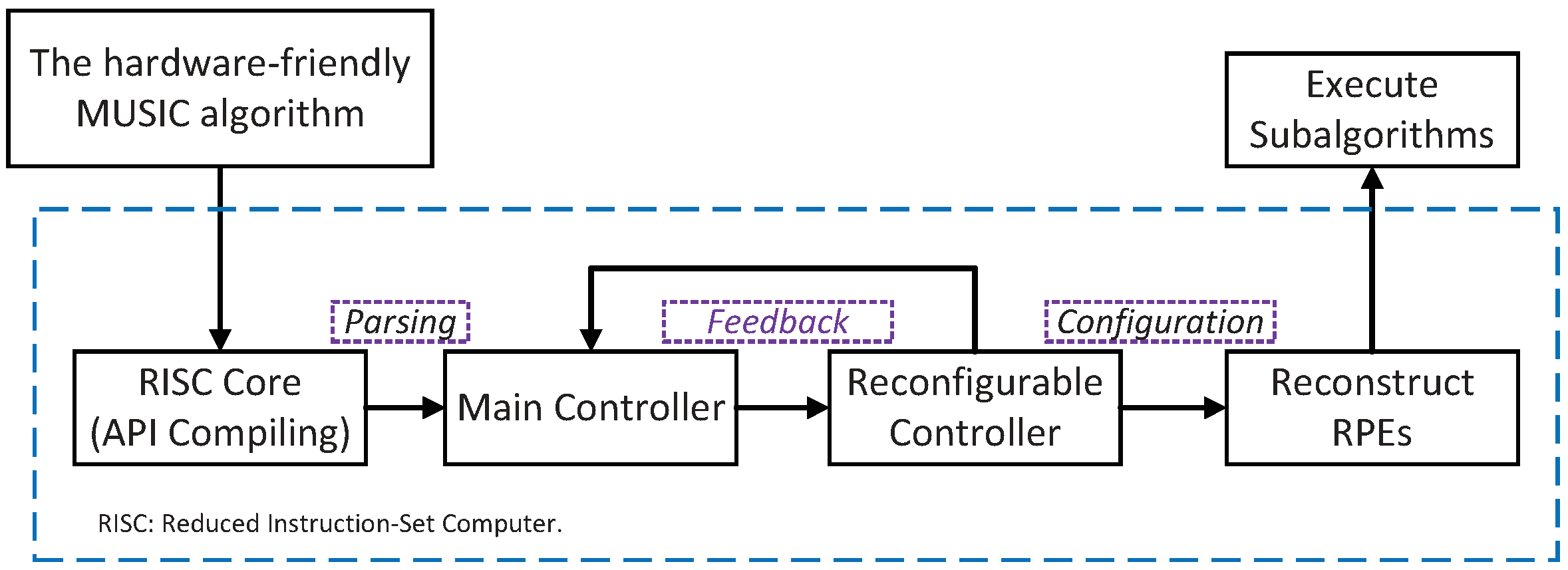
3.1. The Architecture of the Accelerator

The accelerator can speed up the specific algorithms to implement the HFMA, which includes matrix covariance, matrix multiply, matrix addition, direction vector computing (DVC), and spatial spectrum function calculating (SSFC). The detailed architecture of the accelerator is presented below.

From Figure 1, we know that the accelerator consists of a reconfigurable computation array (RCA), a reconfigurable controller (RC), a main controller (MC), a direct memory access (DMA) unit, an AXI interface and an on-chip memory. The RCA has four reconfigurable processing elements (RPEs), and they have identical computational resources, which are listed in Figure 1. The RC manages the computation process and constructs the data paths between memory and RCA. The MC controls the accelerator that includes instruction decoding, DMA configuration, and RC configuration. The DMA and the AXI interface are used to exchange data between off-chip and on-chip memory. The memory has a capacity of 512 KB, and it is divided into 16 banks for high bandwidth and the parallelism requirement.

The accelerator needs to be booted through an external host processor, and we developed an API (application programming interface) function library for the host processor. Once the host processor executes the API, configuration information will be generated. The configure process of HFMA is shown in Figure 2. Firstly, the input HFMA application is described in a high-level language. Then, the code is programmed and compiled by the host processor, which can generate bit streams written to external memory. The accelerator can get the configuration information directly from the host processor or fetch it from external memory initiatively, then the MC receives and translates it to determine which sub-algorithm to be executed. The RC will assign the configure port in RPEs once the particular sub-algorithm is chosen, and the interconnection between the RPEs will be reconfigured meanwhile.

3.2. Implementation of Correlation Matrices’ Estimation

In this section, we propose an implementation method based on the partition to calculate the covariance matrix, which is the first step of HFMA implementation. From Equation (6), it is obvious that the estimate of the array covariance matrix is a calculation of matrix multiplication, but the covariance matrix is a conjugate symmetric matrix in fact. Therefore, $X{X}^H$ can be converted to the following formula:

$$X{X}^H=R_{new}(a,b)=\left\{\begin{array}{cc}X(a,:)·X^{*}(b,:),\hfill & a\ge b,\hfill \\ R_{new}^{*}(a,b),\hfill & a<b,\hfill \end{array}\right.$$

(10)

where $1\le a\le A$, $1\le b\le B$, A is the row number, and B is the column number of the matrix to be solved. When $a\ge b$, the lower triangular results of the covariance matrix can be obtained, while the upper triangular results are obtained by the conjugate symmetry property, which can greatly reduce the computation amount and improve the calculation speed.

The way of storing the source data is shown in Figure 3.

Firstly, we partitioned the banks to be D zones and $D=floor(BS/A)$, where $BS$ is the depth of each bank. Each column of the matrix to be solved is stored in one bank successively. Considering that the maximum number of points of the lower triangular results is $A(A+1)/2$, it takes at least $P=A(A+1)/2/BS$ banks to store these data. The remaining E banks are used to store the source data. Of course, the parallelism of the computation is also subject to the constraint of computing resources. When the matrix size exceeds the maximum storage in a single time, the ping-pong operation will be adopted to carry out multiple data transmission, which can reduce the waiting period for data transportation. This method only needs to write the result back once, and it can reduce the data access time from on-chip to off-chip compared with matrix multiplication. The ping-pong operation for computing the covariance matrix in this architecture is shown in Figure 4.

There exist two address mapping mechanisms to compute the covariance matrix: source data storage and conjugate symmetry of the lower triangular matrix.

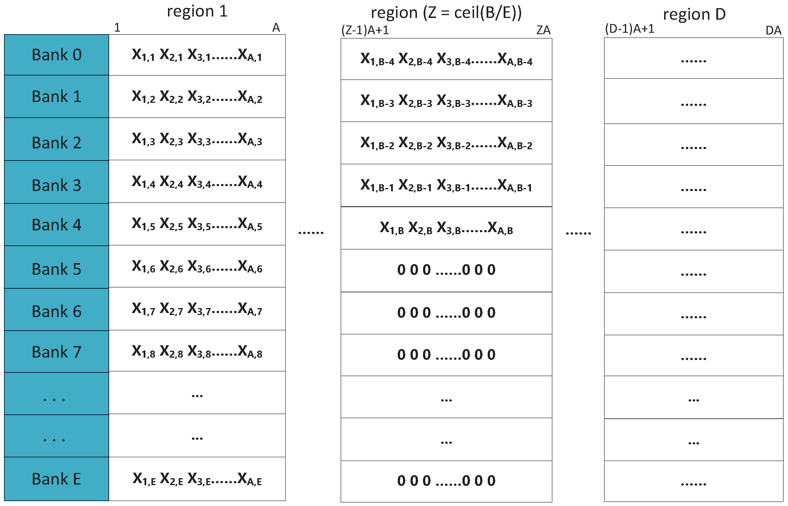
• Source data storage: The data of the matrix to be solved will be numbered from left to right and from top to bottom. Then, the data will be transmitted to the banks in order of increasing number. The address mapping formula is:

  $$\begin{array}{c}matrix\_row=addrX÷COL,\hfill \\ matrix\_column=addrX\%COL,\hfill \\ bank\_num=matrix\_column\%E,\hfill \\ bank\_addr=(matrix\_column÷E)\times COL+matrix\_row,\hfill \end{array}$$

  (11)

  where $addrX$ is the number of data and $COL$ is the column number of the matrix to be solved.
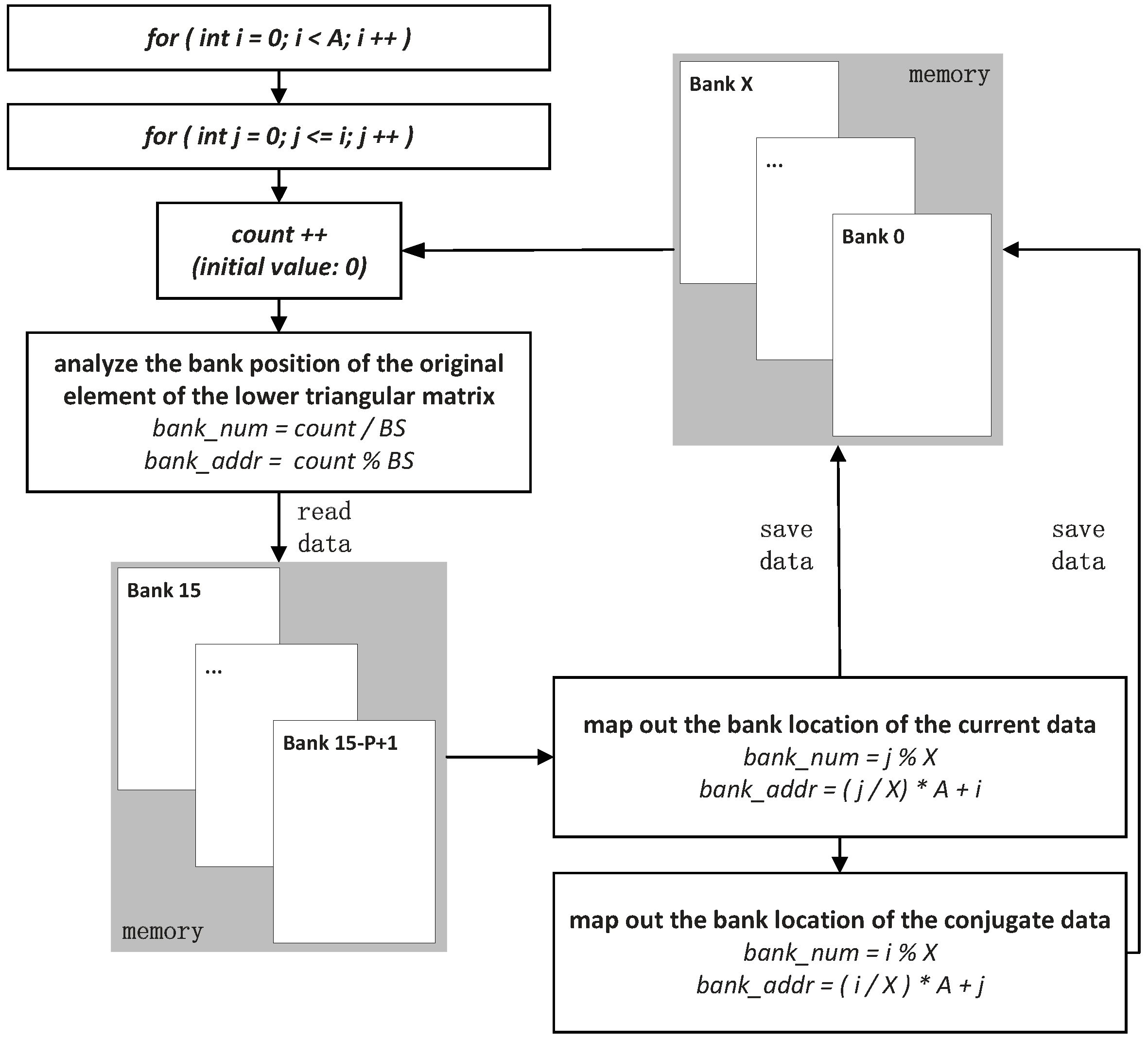
• Conjugate symmetry of the lower triangular matrix: The data of the lower triangular matrix are saved into banks according to the number from top to down and from left to right. In order to obtain the upper triangular matrix, it is necessary to determine the specific location of the original lower triangular matrix in the bank first and then extract the data. The data and its conjugate data are stored in new banks in a manner similar to the mapping mechanism of source data storage. The so-called new banks are actually the original banks of storing the source data, and their reuse scope is from Bank 0 to bank $(15-P+1)$. The specific mapping mechanism is shown in Figure 5.

Based on the above design scheme, we can get the right output with one covariance matrix estimating time of less than 3 μs.

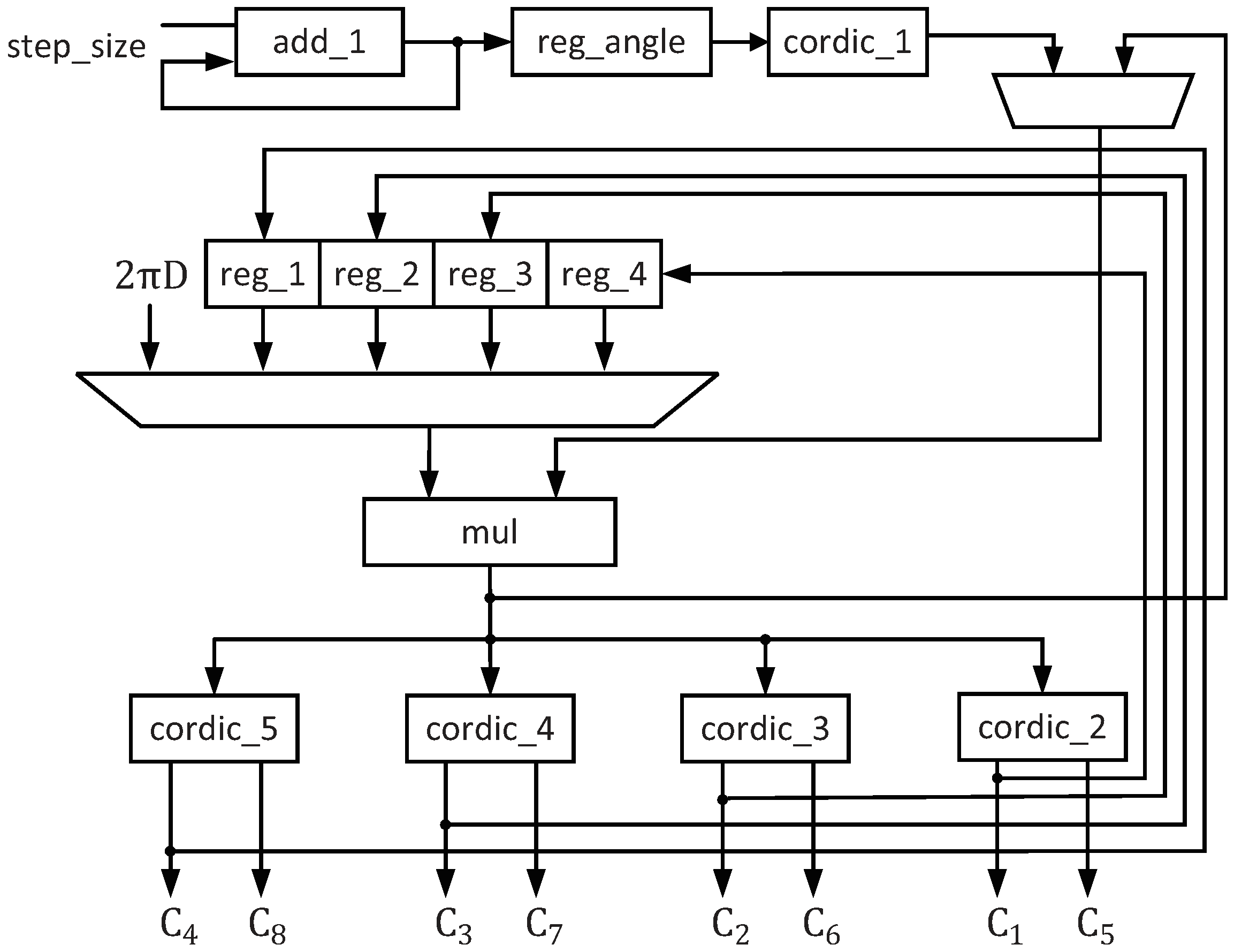
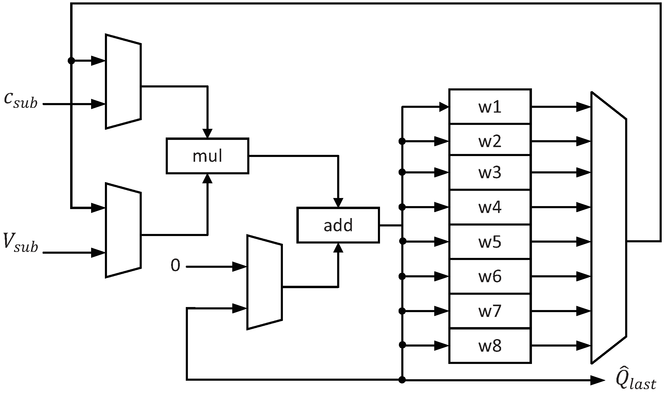
3.3. Implementation of Spectral Peak Search

Spectral peak search is the last step of the HFMA. The direction of the incident signal is obtained by searching the extremum point of the spatial spectral function. The existing research uses a single-step search method to consider search accuracy directly as a search step. When the accuracy requirement is not high, the method is simple and easy to implement. However, when the accuracy requirement increases, the overall calculation will increase dramatically, and the real-time performance decreases significantly. In this paper, we utilized the continuity of the spatial spectrum function to reduce the overall calculation, which is to set a large step for a rough search firstly and then to do the exact search after the first search result.

The most commonly-used method to realize spectrum peak search is based on the look-up table, that is the direction vectors required for spectrum peak search are stored in advance, and the required value is directly read from the memory when constructing the spatial spectrum function. However, the cost of directly using the SRAM is too high, so this paper designs a special hardware circuit to calculate the direction vectors in real time, which not only saves much storage resource when the accuracy requirement is high, but also avoids the adverse impact of reading data on the real-time performance of spectral peak search. The calculation formula of the direction vector is as Equation (7) in the HFMA.

The hardware structure of the module to compute the direction vector is shown in Figure 6. D is the ratio of the wavelength to the radius of the array. $add\_1$ (adder) is used to calculate the radian values of the azimuth angle or the pitch angle, and the result is stored in $reg\_angle$ (register). $cordic\_1$, $cordic\_2$, $cordic\_3$, $cordic\_4$, and $cordic\_5$ are five trigonometric function units, which calculate the values of the sine and cosine functions based on the CORDIC (coordinated rotation digital computer) algorithm. $mul$ (multiplier) is used to complete the multiplication in Equation (7), and $reg\_1$, $reg\_2$, $reg\_3$, and $reg\_4$ (register) store some of the intermediate results of the calculation.

According to Equation (9), the calculation formula of the spatial spectral function is deformed into:

$$\begin{array}{c}w=c_{sub}(M-Q,{\alpha }_q)V_{sub},\hfill \\ {\widehat{Q}}_{last}=\sum _{k=1}^K{w}_k^2,\hfill \end{array}$$

(12)

where ${\widehat{Q}}_{last}$ is the value of the spatial spectral function after deformation. The first step is to execute the multiply-accumulate operation, and the second step is to perform the square-summation operation. When the number of array elements is eight, the hardware structure of the module to calculate the values of the spatial spectrum function is as shown in Figure 7.

This module mainly includes one multiplier and one adder. The multiply-accumulate and the square-summation operation share a set of arithmetic units to save computing resources. The results calculated in Step 1 are cached in eight registers: $w1$, $w2$, …, $w8$. When the number of signal sources changes, only the time of performing the multiply-accumulate operation in the second step needs to be changed, but the hardware structure does not have to be changed.

The block diagram of the spectrum peak search is shown in Figure 8, including the direction vector computing module (DVCM), the spatial spectrum function calculating module (SSFCM), extreme value check module (EVCM), and result store module (RSM). RSM is used to cache the intermediate results of the search step with 1°. When the precision requirement is 1°, directly consider the results as the output. However, when the accuracy requirement is 0.1°, DVCM, SSFCM, and EVCM will perform a precise search with a step size of 0.1° in the surroundings according to the result of the cache.

4. The Experimental Results and Analysis

Currently, almost all the hardware implementations of the MUSIC algorithm use DSP or FPGA architecture. However, this paper realized it based on an efficient and reconfigurable accelerator (ERA), and the results of the experiment will be compared with the DSP implementation in [15] and the FPGA implementation in [16,23].

According to the needs of our practical application scenarios, the achieved DOA precision needs to be compatible with 1° or 0.1°, which are also the most commonly-used precisions. In this paper, we chose the implementations of 0.1° and the other precisions to compare the calculation amount and computation time of the MUSIC algorithm.

Firstly, in order to evaluate the precision of spectral peak search, assume that the case is an eight-element uniform linear array, a single signal source, and 128 snapshots. The experimental results by ERA are shown in

Table 2. The experimental results of direction estimates.

Exp #	The Azimuth Angle (°)			or		The Pitch Angle (°)
	Input	Output	Error ($\mathbf{\Delta }\mathit{\theta }$)		Input		Output	Error ($\mathbf{\Delta }\mathit{\theta }$)
1	${10}^{\circ }$	${9.97}^{\circ }$	${0.03}^{\circ }$		$0^{\circ }$		${0.05}^{\circ }$	${0.05}^{\circ }$
2	${50}^{\circ }$	${50.02}^{\circ }$	${0.02}^{\circ }$		${10}^{\circ }$		${9.93}^{\circ }$	${0.07}^{\circ }$
3	${90}^{\circ }$	${89.96}^{\circ }$	${0.04}^{\circ }$		${20}^{\circ }$		${20.02}^{\circ }$	${0.02}^{\circ }$
4	${130}^{\circ }$	${130.01}^{\circ }$	${0.01}^{\circ }$		${30}^{\circ }$		${30.06}^{\circ }$	${0.06}^{\circ }$
5	${170}^{\circ }$	${170.03}^{\circ }$	${0.03}^{\circ }$		${40}^{\circ }$		${40.01}^{\circ }$	${0.01}^{\circ }$
6	$-{10}^{\circ }$	$-{10.05}^{\circ }$	${0.05}^{\circ }$		${50}^{\circ }$		${50.05}^{\circ }$	${0.05}^{\circ }$
7	$-{50}^{\circ }$	$-{50.01}^{\circ }$	${0.01}^{\circ }$		${60}^{\circ }$		${59.97}^{\circ }$	${0.03}^{\circ }$
8	$-{90}^{\circ }$	$-{90.02}^{\circ }$	${0.02}^{\circ }$		${70}^{\circ }$		${70.02}^{\circ }$	${0.02}^{\circ }$
9	$-{130}^{\circ }$	$-{130.03}^{\circ }$	${0.03}^{\circ }$		${80}^{\circ }$		${80.01}^{\circ }$	${0.01}^{\circ }$
10	$-{170}^{\circ }$	$-{170.02}^{\circ }$	${0.02}^{\circ }$		${90}^{\circ }$		${90.05}^{\circ }$	${0.05}^{\circ }$

Exp #: experimental serial number.

, and it proves the effectiveness of the HFMA (the precision requirement was 0.1°).

It can be seen from the values of error angle $\Delta \theta$ in Table 2 that the hardware system can satisfy the 0.1° resolution requirements. The experiments completed the spectrum peak search in the first step by 1°, and then near the results of the first step, the second step would try to search many times until an accurate result was obtained. Then, we further explored the probability of resolution [24] and performed 500 trials to compute it. Figure 9 shows the probability of the resolution under two different DOA precisions, which can also prove the effectiveness of the HFMA.

Next, this reconfigurable accelerator had a significant advantage in the total time of implementing the MUSIC algorithm. Compared with the implementations of [15,16,23], the accelerator took far less time to complete the MUSIC algorithm, which can meet the requirements of the high real-time applications. Based on the above input case: an eight-element uniform linear array, a single signal source, and 128 snapshots, the calculation time of the MUSIC algorithm was as shown in

Table 3. Comparison among different implementations.

		Item	ECM 1	FDCM 2	SPS 3	Total Periods
	Computation Period
Components
(DSP) Reference [15]/(MHz)			28,000/(124.3)	110,000/(124.3)	36,000/(124.3)	174,000/(124.3)
(FPGA) Reference [16]/(MHz)			8032/(160)	8064/(160)	4464/(160)	20,560/(160)
(FPGA) Reference [23]/(MHz)			4096/(119.8)	52,000/(105.4)	31,500/(128.6)	87,596/(105.4)
(FPGA) This paper/(MHz)			2800/(145)	/	22,700/(145)	25,500/(145)
First Speed-up Ratio 4			90.0%	/	36.9%	85.3%
Second Speed-up Ratio 5			65.1%	/	−80.3%	−19.3%
Third Speed-up Ratio 6			31.6%	/	11.4%	74.5%

¹ ECM: estimation of covariance matrix. ² FDCM: feature decomposition of covariance matrix. ³ SPS: spectral peak searching. ⁴ This paper vs. [15]. ⁵ This paper vs. [16]. ⁶ This paper vs. [23].

. Regarding to the speed-up ratio, the calculation formula was $\frac{C{P}_{ref}-C{P}_{pro}}{max\{C{P}_{ref},C{P}_{pro}\}}$, where $C{P}_{ref}$ represents the computation period in the reference paper and $C{P}_{pro}$ represents the computation period in this paper.

Through the above experimental results, we know that the implementation of the HFMA based on the accelerator is effective and the computation period of the MUSIC algorithm is shorter than [15,23]. Although the second speed-up ratios of SPS and TET were −80.3% and −19.3%, which shows that the computation period in [16] was shorter than that in this paper, the average error was 0.6° in [16], while in this paper, it was 0.1°. The smaller the average error, the longer the spectral peak search time to obtain the accuracy by the stepwise search method. Actually, in terms of calculating the covariance matrix, the second speed-up ratio was 65.1%, where the paper obviously had an advantage.

However, in order to better compare with [16,23] and explain the advantages of the proposed accelerator under the same experiment platform, we also used the Virtex-6 development board for resource assessment. The specific resource usage is shown in

Table 4. Different implementations in FPGA.

	Design	Reference [16]	Reference [23]	This Paper
Item
Device Type		Virtex-6	Virtex-6	Virtex-6
Max Frequency		160 MHz	105.451 MHz	145 MHz
LUTs		54,100	45,374	48,060
Registers		92,200	/	30,216
DSP48E1		64	241	96
Block RAM		/	270 KB	512 KB
Equivalent Slices		13,957	15,384	18,236
Precision		${0.6}^{\circ }$	${0.1}^{\circ }$	$1^{\circ }$ or ${0.1}^{\circ }$

. In order to make the area usage evaluation of FPGA more accurate, all resources were firstly equaled to LUTs and registers and then further measured by slice. According to the Virtex-6 product specification [25], one LUT can be equivalent to one 64-bit BRAM. However, there is no equivalent relation about one DSP48E1 and LUTs (or registers) in the product specification, so we evaluated it by the following method. We re-instantiated all the IPs of DSP48E1 and prioritized fewer DSP48E1 over all DSP48E1 to make DSP48E1 usage decrease from 96 to 64. Then, the result showed that the LUTs and registers were 4128 and 3200 more than before, respectively. Therefore, we think that the one DSP48E1 equaled 129 LUTs and 100 registers. Secondly, from [25], we know that one slice consists of four LUTs and eight registers. Therefore, all resources would be equal to the slices. The equivalent slices of different implementations are shown in Table 4. In order to weigh and compare the performance of different implementation methods, the following standard metric was used in this paper, and the results are shown in

Table 5. Performance comparison after normalization.

	Design	This Paper vs. Reference [16]	This Paper vs. Reference [23]
Item
$C{P}_r$		0.81	3.44
$Slic{e}_r$		1.3	1.18
$B{P}_r$		0.623	2.915

. That is:

$$B{P}_r=\frac{C{P}_{ref}÷C{P}_{pro}}{Slic{e}_{pro}÷Slic{e}_{ref}}=\frac{C{P}_r\left(\mathrm{performance}\mathrm{ratio}\right)}{Slic{e}_r\left(\mathrm{area}\mathrm{ratio}\right)},$$

(13)

where $B{P}_r$ represents the balanced performance ratio, $C{P}_{ref}$ stands for the computation periods of the reference (performance), $Slic{e}_{ref}$ stands for the slices of the reference (area), $C{P}_{pro}$ stands for the computation periods of this paper (performance), $Slic{e}_{pro}$ stands for the slices of this paper (area), $C{P}_r$ stands for the computation period ratio, and $Slic{e}_r$ stands for the slice ratio. Therefore, if $B{P}_r$ is greater than one, the performance of the proposed method is excellent, and greater $B{P}_r$ means better performance. If $B{P}_r$ is equal to one, the performance of the two methods is equal. If $B{P}_r$ is less than one, the performance of the other method is dominant.

From Table 5, we can see that the $B{P}_r$s were 0.623 and 2.915, respectively, which indicates that the performance of the proposed method was better than that of [23]. Although $B{P}_r=0.623$ shows that the performance (computation periods per slice) decreased by 37.7% compared to [16], the precision of spectral peak search also played a great role in the performance. The higher the accuracy requirement, the longer the spectral peak search time. Consider that the average error was 0.6° in [16], while that in this paper was 0.1°, despite that the precision cannot be accurately associated with $B{P}_r$. It is closely related to the SPS module. From the references [15,23], even including the proposed accelerator, we know that the computation period of SPS was 8.06×, 7.06×, and 5.08× more than that in [16] to achieve the 0.1° precision, respectively. Therefore, even if the [16] used the SPS of the minimum computation period (this paper) among them in order to reach 0.1° precision, its total periods would be 38,796, in which case, $B{P}_r$ (this paper vs. [16]) would be 1.17, which would increase the performance by 17% and further indicate that the proposed accelerator had a certain dominance.

Besides, as for the applications of the more challenging scenarios [24,26,27,28,29], the proposed accelerator to implement the HFMA is still useful or can be further improved. Taking the application of the TR-MUSIC (time-reversal MUSIC) algorithm [27,28,29] as an example, the operations mainly include matrix multiplication, matrix addition, matrix inversion, and matrix covariance. The proposed accelerator in this paper can exactly speed up the above operations except for matrix inversion. However, due to the great flexibility of the reconfigurable architecture, a matrix inversion module can be designed on the basis of not changing the existing architecture and considered as a sub-algorithm to be added to the RC shown in Figure 1. Since the accelerator works in cooperation with the external host processor, the application of the TR-MUSIC algorithm will be described in a high-level language. Then, the host processor compiles the code and transmits the operation instructions mentioned above to the reconfigurable accelerator. The accelerator receives the instructions and executes these specific sub-algorithms to speed up the application of the TR-MUSIC algorithm. The specific configuration process is similar to that shown in Figure 2. With regard to the applications of these challenging scenarios, further research can be done to make the reconfigurable accelerator more versatile, so as to meet the requirements of different application scenarios.

5. Conclusions

In this paper, the implementation of HFMA based on an efficient and reconfigurable architecture was proposed. The implementation process was mainly divided into two steps: Firstly, we optimized the MUSIC algorithm to avoid the eigenvalue decomposition of the covariance matrix. Then, we implemented the correlation matrices estimation and spectral peak search in the reconfigurable architecture. Our implementation can better speed up the MUSIC algorithm to meet the high real-time capability for the DOA estimation and be compatible with both the 1° and 0.1° accuracy requirements. Synthesized under the TSMC 40-nm CMOS technology with the Synopsys Design Compiler, we obtained a maximum frequency of 1 GHz with a 4,765,475.4 μm² area, and the power dissipation was 238.27 mW. The experimental results showed that the total time of the MUSIC algorithm was 25.5 μs at the frequency of 1 GHz, which was better than some previously-published work.

In the future, we will exploit the proposed architecture to estimate the number of sources, which is a necessary pre-requisite for spectral-based DOA methods. We envision that we can preset a threshold value and compare the increasing range of all eigenvalues of the covariance matrix with it. If the increasing range of two eigenvalues is less than the threshold, the eigenvalues are considered as noise eigenvalues. When the increasing range of the two eigenvalues is greater than the threshold for the first time, it indicates that the two eigenvalues are the first signal eigenvalue and the last noise eigenvalue, so that the number of sources can be determined. Based on the above idea, we can further study whether the proposed architecture can be used to optimize the algorithm after adding the threshold value, so as to achieve the goal of reducing the computation amount. Besides, we can further study whether the proposed HFMA is useful for other array structures.

References

1. Schmidt, R. Multiple Emitter Location and Signal Parameter Estimation. IEEE Trans. Antennas Propag. 1986, 3, 276–280. [Google Scholar] [CrossRef]
2. Zoltowski, M.D.; Kautz, G.M.; Silverstein, S.D. Beamspace Root-MUSIC. IEEE Trans. Signal Process. 1993, 41, 344. [Google Scholar] [CrossRef]
3. Ren, Q.S.; Willis, A.J. Fast root MUSIC algorithm. Electron. Lett. 1997, 33, 450–451. [Google Scholar] [CrossRef]
4. He, Z.S.; Li, Y.; Xiang, J.C. A modified root-music algorithm for signal DOA estimation. J. Syst. Eng. Electron. 1999, 10, 42–47. [Google Scholar]
5. Cheng, Q.; Lei, H.; So, H.C. Improved Unitary Root-MUSIC for DOA Estimation Based on Pseudo-Noise Resampling. IEEE Signal Process. Lett. 2014, 21, 140–144. [Google Scholar]
6. Chen, Q.; Liu, R.L. On the explanation of spatial smoothing in MUSIC algorithm for coherent sources. In Proceedings of the International Conference on Information Science and Technology, Nanjing, China, 26–28 March 2011; pp. 699–702. [Google Scholar]
7. Iwai, T.; Hirose, N.; Kikuma, N.; Sakakibara, K.; Hirayama, H. DOA estimation by MUSIC algorithm using forward-backward spatial smoothing with overlapped and augmented arrays. In Proceedings of the International Symposium on Antennas and Propagation Conference Proceedings, Kaohsiung, Taiwan, 2–5 December 2014; pp. 375–376. [Google Scholar]
8. Wang, H.K.; Liao, G.S.; Xu, J.W.; Zhu, S.Q.; Zeng, C. Direction-of-Arrival Estimation for Circulating Space-Time Coding Arrays: From Beamspace MUSIC to Spatial Smoothing in the Transform Domain. Sensors 2018, 11, 3689. [Google Scholar] [CrossRef] [PubMed]
9. Zhao, Q.; Dong, M.; Liang, W.J. Research on modified MUSIC algorithm of DOA estimation. Comput. Eng. Appl. 2012, 48, 102–105. [Google Scholar]
10. Hong, W. An Improved Direction-finding Method of Modified MUSIC Algorithm. Shipboard Electron. Countermeas. 2011, 34, 71–73. [Google Scholar]
11. Wang, F.; Wang, J.Y.; Zhang, A.T.; Zhang, L.Y. The Implementation of High-speed parallel Algorithm of Real-valued Symmetric Matrix Eigenvalue Decomposition through FPGA. J. Air Force Eng. Univ. 2008, 6, 67–70. [Google Scholar]
12. Kim, Y.; Mahapatra, R.N. Dynamic Context Compression for Low-Power CoarseGrained Reconfigurable Architecture. IEEE Trans. Very Large Scale Integr. (VLSI) Syst. 2010, 18, 15–28. [Google Scholar] [CrossRef]
13. Hwang, W.J.; Lee, W.H.; Lin, S.J.; Lai, S.Y. Efficient Architecture for Spike Sorting in Reconfigurable Hardware. Sensors 2013, 11, 14860–14887. [Google Scholar] [CrossRef] [PubMed]
14. Wang, S.J.; Liu, D.T.; Zhou, J.B.; Zhang, B.; Peng, Y. A Run-Time Dynamic Reconfigurable Computing System for Lithium-Ion Battery Prognosis. Energies 2016, 8, 572. [Google Scholar] [CrossRef]
15. Li, M.; Zhao, Y.M. Realization of MUSIC Algorithm on TMS320C6711. Electron. Warf. Technol. 2005, 3, 36–38. [Google Scholar]
16. Yan, J.; Huang, Y.Q.; Xu, H.T.; Vandenbosch, G.A.E. Hardware acceleration of MUSIC based DoA estimator in MUBTS. In Proceedings of the 8th European Conference on Antennas and Propagation, The Hague, The Netherlands, 6–11 April 2014; pp. 2561–2565. [Google Scholar]
17. Sun, Y.; Zhang, D.L.; Li, P.P.; Jiao, R.; Zhang, B. The studies and FPGA implementation of spectrum peak search in MUSIC algorithm. In Proceedings of the International Conference on AntiCounterfeiting, Security and Identification, Macao, China, 12–14 December 2014. [Google Scholar]
18. Deng, L.K.; Li, S.X.; Huang, P.K. Computation of the covariance matrix in MSNWF based on FPGA. Appl. Electron. Tech. 2007, 33, 39–42. [Google Scholar]
19. Wu, R.B. A novel universal preprocessing approach for high-resolution direction-of-arrival estimation. J. Electron. 1993, 3, 249–254. [Google Scholar]
20. TMS320C6672 Multicore Fixed and Floating-Point DSP (2014) Lit. No. SPRS708E; Texas Instruments Inc.: Dallas, TX, USA, 2014.
21. TMS320C66x DSP Library (2014) Lit. No. SPRC265; Texas Instruments Inc.: Dallas, TX, USA, 2014.
22. Yu, J.Z.; Chen, D.C. A fast subspace algorithm for DOA estimation. Mod. Electron. Tech. 2005, 12, 90–92. [Google Scholar]
23. Huang, K.; Sha, J.; Shi, W.; Wang, Z.F. An Efficient FPGA Implementation for 2-D MUSIC Algorithm. Circuits Syst. Signal Process. 2016, 35, 1795–1805. [Google Scholar] [CrossRef]
24. Wang, M.Z.; Nehorai, A. Coarrays, MUSIC, and the cramer–rao bound. IEEE Trans. Signal Process. 2017, 65, 933–946. [Google Scholar] [CrossRef]
25. Virtex-6 Family Overview. Available online: http://www.xilinx.com/support/documentation/data_sheets/ds150.pdf (accessed on 8 May 2019).
26. Devaney, A.J. Time reversal imaging of obscured targets from multistatic data. IEEE Trans. Antennas Propag. 2005, 53, 1600–1610. [Google Scholar] [CrossRef]
27. Ciuonzo, D.; Romano, G.; Solimene, R. On MSE performance of time-reversal MUSIC. In Proceedings of the IEEE 8th Sensor Array and Multichannel Signal Processing Workshop (SAM), A Coruna, Spain, 22–25 June 2014. [Google Scholar]
28. Ciuonzo, D.; Romano, G.; Solimene, R. Performance analysis of time-reversal MUSIC. IEEE Trans. Signal Process. 2015, 63, 2650–2662. [Google Scholar] [CrossRef]
29. Ciuonzo, D.; Rossi, P.S. Noncolocated time-reversal MUSIC: high-SNR distribution of null spectrum. IEEE Signal Process. Lett. 2017, 24, 397–401. [Google Scholar] [CrossRef]
Figure 1. The architecture of the accelerator.
Electronics 08 00511 g001
Figure 2. The configuration process of the accelerator.
Electronics 08 00511 g002
Figure 3. The way of storing the source data.
Electronics 08 00511 g003
Figure 4. Ping-pong operation for computing the covariance matrix. PE, processing element.
Electronics 08 00511 g004
Figure 5. Address mapping mechanism of the conjugate symmetry of lower triangular matrix.
Electronics 08 00511 g005
Figure 6. The hardware structure of the direction vector computing module.
Electronics 08 00511 g006
Figure 7. The hardware structure of the spatial spectrum function calculating module.
Electronics 08 00511 g007
Figure 8. The block diagram of implementing the spectrum peak search.
Electronics 08 00511 g008
Figure 9. Probability of resolution vs. Δ θ .
Electronics 08 00511 g009