Localization and Frequency Identification of Large-Range Wide-Band Electromagnetic Interference Sources in Electromagnetic Imaging System

Abstract

The identification and localization of large-range, wide-band electromagnetic interference (EMI) sources have always been both costly and time-consuming. The measurements at different times and places are often required before a typical system can locate a target. In this paper, we proposed a 2D electromagnetic imaging system to localize interference sources and identify the EMI frequency in real time. In this system, an offset paraboloid with a diameter of three meters is designed for large-range EMI imaging, while a multi-channel digital signal acquisition system is developed for wide-band EMI localization. The located interference source is segmented by the maximum entropy method based on particle swarm optimization, and the modified generalized regression neural network (MGRNN) is applied to identify the EMI frequency effectively by excluding misleading effects of outliers. The experiment which has been completed on our dataset indicates that our approach not only increases accuracy by 5% compared with the standard generalized regression neural network approaches for identification, but also exerts a large-range wide-band localization of the EMI source detection method.

1. Introduction

It is a growing trend that wireless products are spreading tremendously in our life. These wireless systems could be very sensitive to electromagnetic interference (EMI), which could be either generated unintentionally from other electronic systems, or generated intentionally by jammers. Thus, the identification and localization of the radio EMI will be demanded under more circumstances. Such work is classically done with a spectrum analyzer or other qualified measurement equipments. The tikhonov regularization algorithm in conjunction with L-curve method proposed by Anastasia [1] provided a stable inverse reconstruction of the multi-dipole model distribution in the object plane. Salman [2] investigated the performance of a planar elliptical dipole textile antenna for the multi-sensor (impulse GPR & EMI) subsurface detection system. Andrey [3] presented a localization technique for stochastic EMI sources based on time domain measurements of EM near-field tangential components. The autocorrelation and cross-correlation functions obtained by the two-point planar scanning system are used for the characterization of stochastic field distribution. However, such systems require a series of complex measurements for the direct measurements on the device surface at different times and locations.

Such problem of electromagnetic compatibility related to the localization of sources can be solved by using the remote sensing of electromagnetic radiation and imaging of field distribution to the plane of the device under test. Hui He [4,5,6,7] visualized the frequency-dependent electromagnetic field distribution for electromagnetic compatibility (EMC) applications and the time evolution of the current flow induced by an electrostatic discharge (ESD) on complex-shaped electronic systems. Pratik Maheshwari [8,9] presented an emission source microscopy (ESM) technique derived from synthetic aperture radar (SAR) to localize radiating sources on a printed circuit boards (PCB) for large, complex systems with multiple sources at the same frequency. Mojtaba [10] introduced two new techniques for microwave imaging of layered structures. These techniques were developed to address the limits associated with classical SAR imaging techniques to generate focused and properly-positioned images of embedded objects in generally layered dielectric structures. Yang Liu [11,12] proposed a magnetic dipole array-based time-domain (TD) modeling of electromagnetic near-field (NF) radiated by PCB. Blaise Ravelo [13] introduced a fast and simple computational method of 3D near-field radiation from 2D planar frequency and time dependent data. However, these methods only work in a narrow band and small scale for near-field emission. We proposed a 2D electromagnetic imaging system to localize interference sources for wide-band, large-range and far-field.

It is important to recognize the frequency of EMI sources for suppression purposes or image recovery. The frequency of EMI can be identified according to type and statistic feature, as well as the environment in which the source is encountered. In this study, a novel approach based on the artificial neural networks is introduced. The work applies singular value decomposition (SVD) [14,15] and modified SVD [16] to probabilistic neural network (PNN). However, measuring SVD over a block of pixels will inevitably decrease the classification accuracy. GRNN is a “one-pass” neural network without requiring any iterative calculation [17,18]. Therefore, the solution of GRNN could be certain, stable, fast and highly accurate in prediction. By using GRNN, Lu Ning [19] achieved a good result when detecting a target on sea surface. However, such a method requires a large amount of parameters before the system start working and the parameters, which will influence the prediction result, are very time-consuming to acquire by experiment. The MGRNN is able to extract network parameters accurately and effectively to solve this problem.

In this paper, we explored a 2D electromagnetic imaging system for the identification and localization of large-range wide-band EMI sources. Localization was achieved by the electromagnetic imaging hardware system using an offset paraboloid. After the EMI source was located, it was segmented from the image by multi-threshold segmentation. Eventually, the identification of the frequency was implemented by MGRNN.

The paper is organized as follows. Section 2 provides a detailed description of the system architecture for localization of EMI sources. In Section 3, we explain the electromagnetic interference identification using a new algorithm. The experimental results are presented along with discussions in Section 4, followed by conclusions in Section 5 to sum up the presented work.

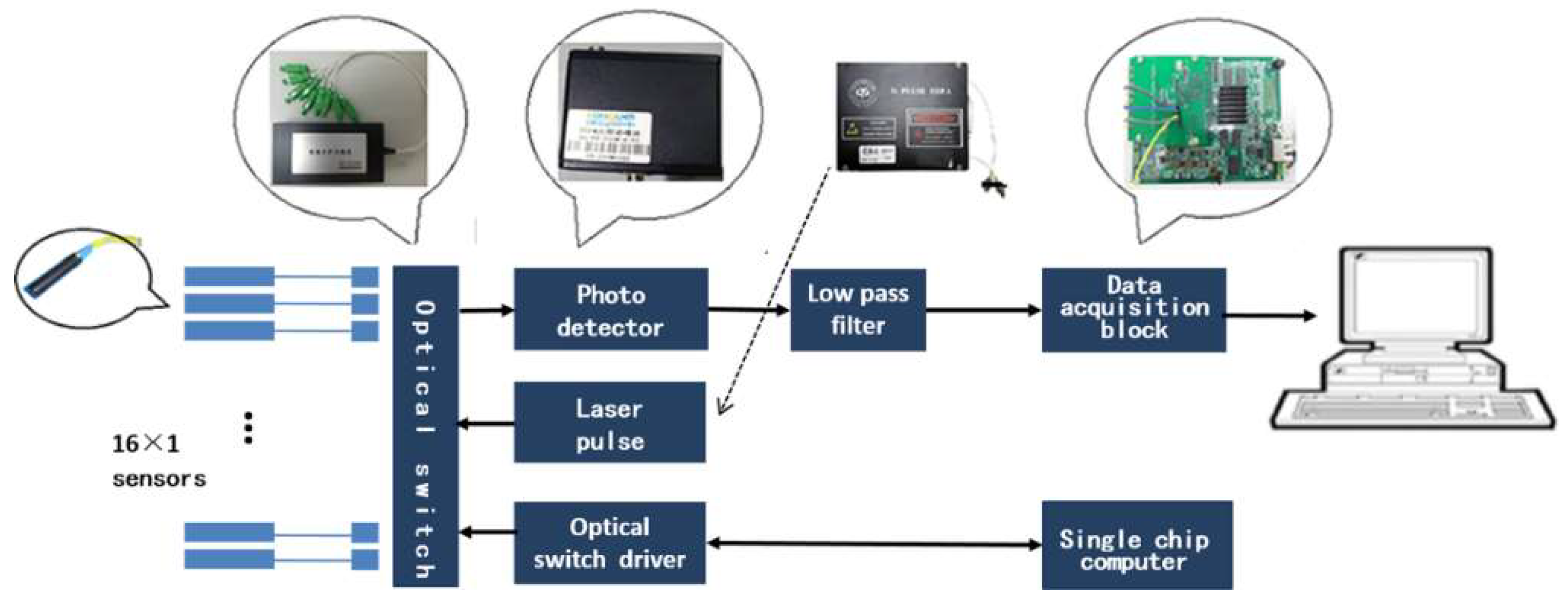
2. System Architecture

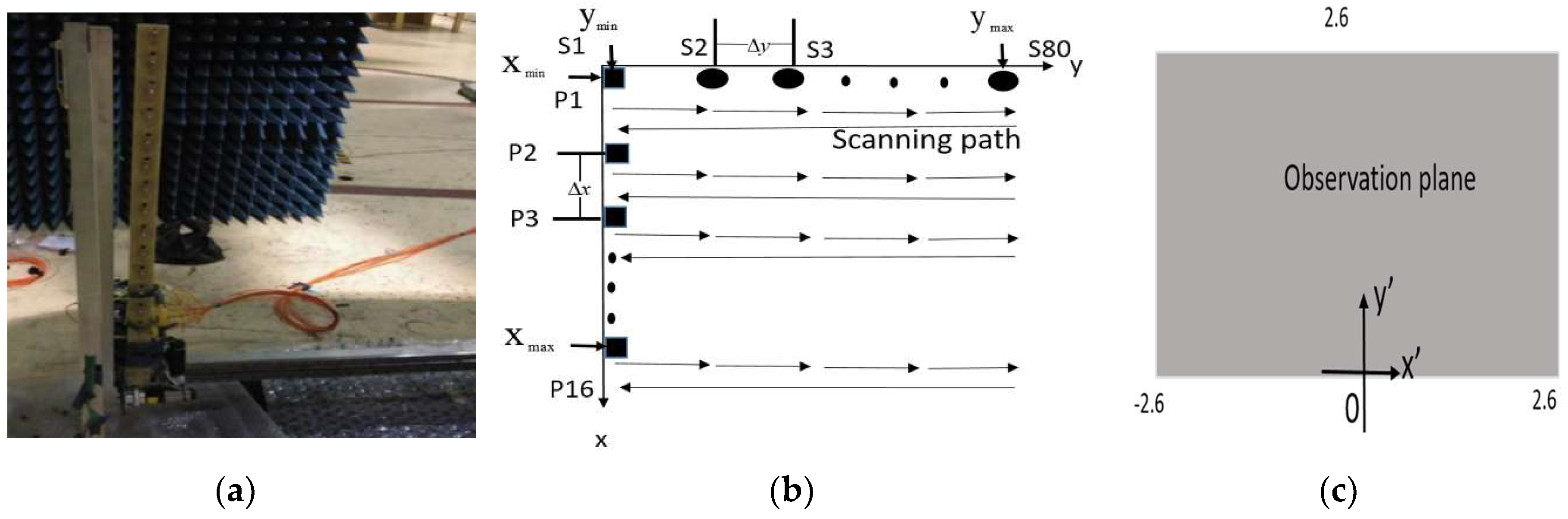
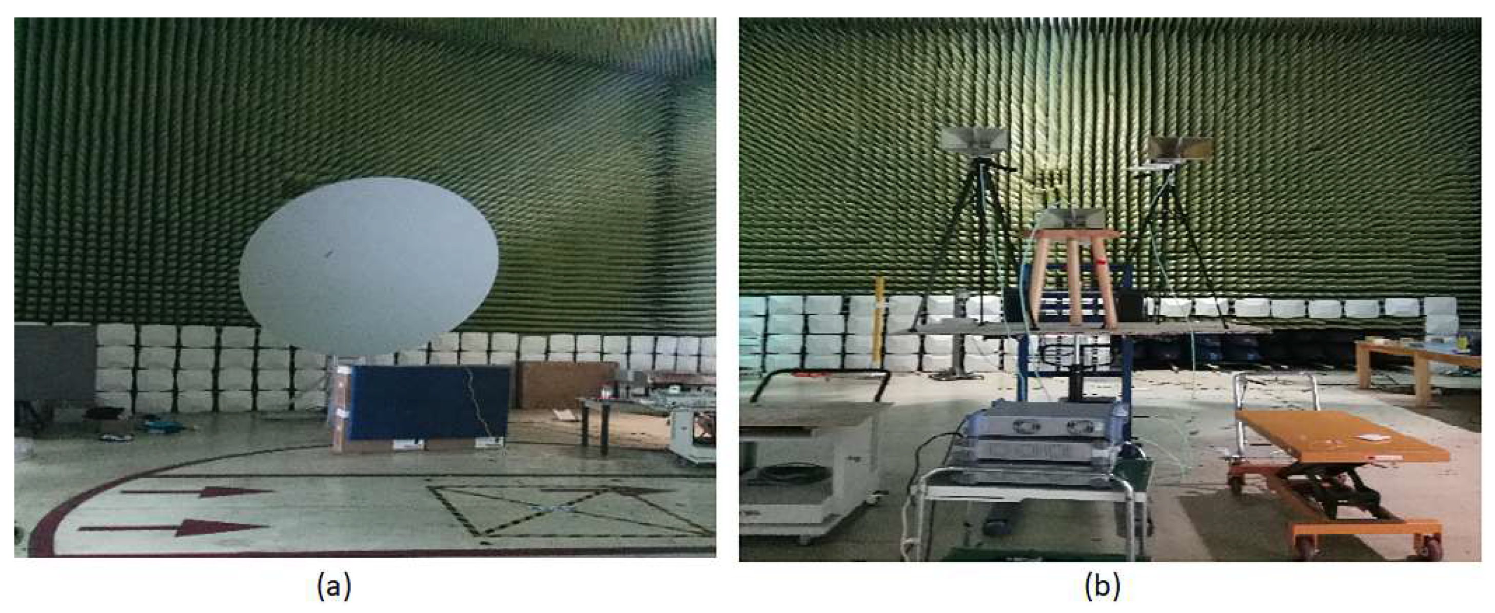
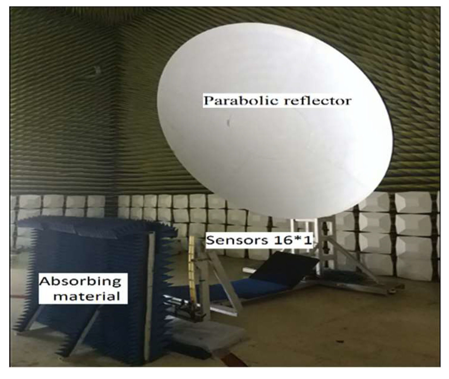
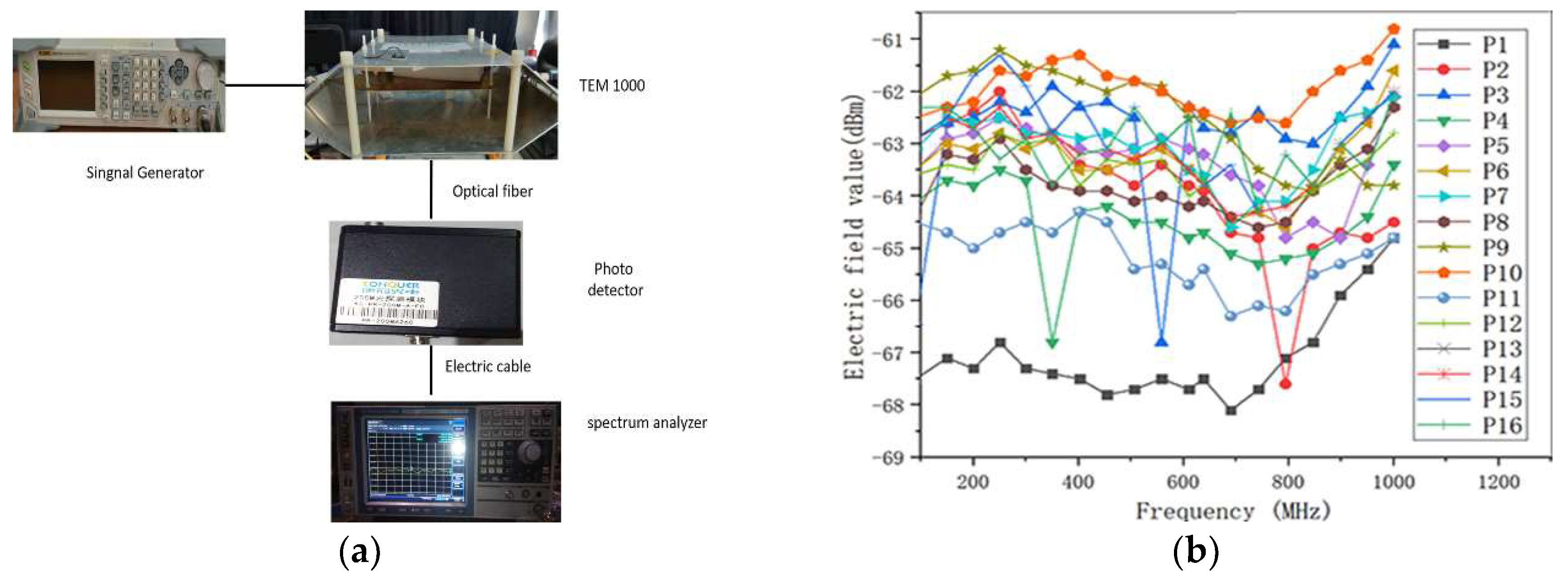
2.1. The Electromagnetic Imaging System

Figure 1 shows the electromagnetic imaging system. We used a reflective surface to achieve the convergence of wide-band electromagnetic waves. The sensors modulated the spatial electric field on an optical signal and then the modulated signal was converted into an electric signal by a photo detector. The optical switch controlled by an optical switch drive and single chip computer could select one output from multiple inputs to the photo detector. The laser pulse provided a pulsed laser with stable frequency and narrow pulse width to optical switch. If the electric field information modulated on the optical signal fell within the working bandwidth of the photo detector, the output voltage signals of the photo detector would have the same frequency as the spatial E-field, and its amplitude would be proportional to the component of the spatial electric field signal. The multi-channel data acquisition block was applied to convert the voltage signal from the photo detector into digital signals, which could be processed and uploaded by a computer.

The laser pulse source is designed and manufactured by School of Electronic and Information Engineering, Beihang University, Beijing, China. The pulse source has a repetition frequency of 52 MHz, a pulse width of several hundred femtoseconds, and a relatively concentrated energy. The wavelength distribution is also substantially concentrated on the specific wavelength 1550 nm.

In order to simplify the system complexity and reduce the system cost, the multi-channel optical switch which is made by Beijing Kangguan Photoelectric Technology Company, China were used to realize the rapid switch the optical path, and it was not necessary to equip the multiple photo detectors in the system. In addition, the optical switch can complete the optical path conversion for a few milliseconds, which helped meet the high efficiency detection requirements of the project.

As a module for converting light signals into the electrical signals, the photo detector which is made by Beijing Kangguan Photoelectric Technology Company, China is the key to achieve wide-band electric field measurements in the entire system. The spectral response range is from 850–1650 nm, which include the 1550 nm, the conversion efficiency is 14.4 kV/W, and the 3-dB bandwidth is 200 MHz.

The multi-channel data acquisition block which is made by Zhongxing Lianhua Technology Company, Beijing, China is composed of two parts: field programmable gate arrays (FPGA) and acorn RISC machine (ARM). The FPGA is used to the 4K points fast Fourier transform (FFT); the ARM is mainly applied for reading/writing the SD card, reading the result of fast Fourier transform calculation from the FPGA and passing the TCP/IP protocol and then the result data is sent to the computer.

An optical electric field sensor which is made by SEIKOH GIKEN Company, Matsudo City, Chiba, Japan is used to convert the electric fields to an optical signal by modulating the E-fields to light and translate it by optical fiber. The sensor probe has a frequency response of 100 kHz to 10 GHz and can detect field levels of 0.01 to 500 V/m.

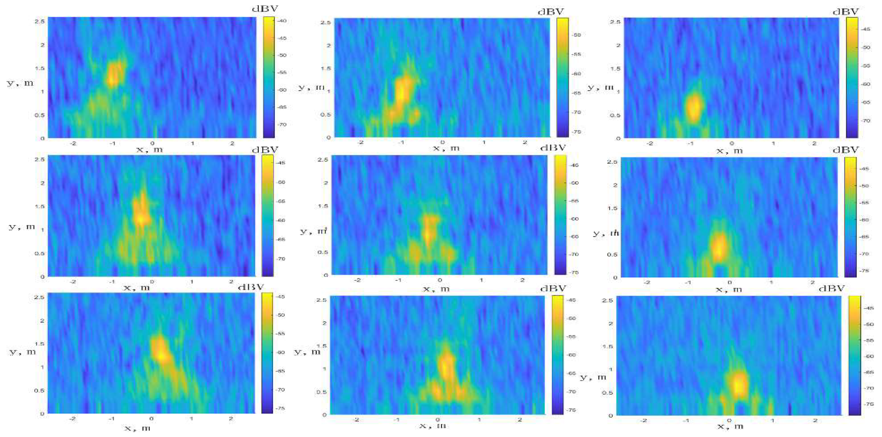
2.2. Large-Range EMI Imaging

Figure 2 Shows the parabolic reflector of the imaging system. It makes the interference source imaging 10 m away from the reflective surface. An offset paraboloid with a diameter of 3 m can realize a large range imaging which is 5.2 m × 2.6 m in rectangular area. The reflective surface is 1.25 m in height from the ground and the receiving surface is offset to reduce aberration. The E-field information is sensed by the sensors. Then, by data processing system, the interference source image is displayed on the computer.

The 16 × 1 probes (P1–P16) are placed at the scanning surface point in Figure 3a. The scan process takes place in a row-wise fashion, i.e., scanning towards the y-axis for 80 points (S1–S80) at each row and moving back to the starting point, as explained in Figure 3b. In the first step, they record the measured data, and then, the probes return back to the origin point P1-P16. As input data of the far field is processing, the E-field components are shown on observation plane in Figure 3c. The far field maps are visualized from the scan plane delimited by x_min = 0 m, x_max = 0.75 m, y_min = 0 m and y_max = 1.2 m, step Δx = 5 cm and Δy = 1.5 cm to the observation plane which is x’_min = −2.6 m, x’_max = 2.6 m and y’_min = 0 m, y’_max = 2.6 m.

The transverse electromagnetic (TEM) cell can be used to measure response characteristics of each sensor and the block diagram illustrating the test bench is described in Figure 4a. With this test bench, the path of the data flow can also be observed. The test bench is composed of the signal generator, E-field probe, TEM cell, light detection circuit, and spectrum analyzer. The signal generator was applied to output the same signal power value to the TEM cell. The probe was placed in the TEM cell to modulate the spatial electric field on an optical signal, then the modulated optical signal was converted into an electric signal by a photo detector. At last, the spectrum analyzer could obtain the electric signal power value. As can be seen from Figure 4b, the input signals had the same power value of −5 dBm in different frequencies in the test bench, and the response characteristics of the sensors could be obtained. The results show the fluctuation range of 4 dBm from the 16 probes.

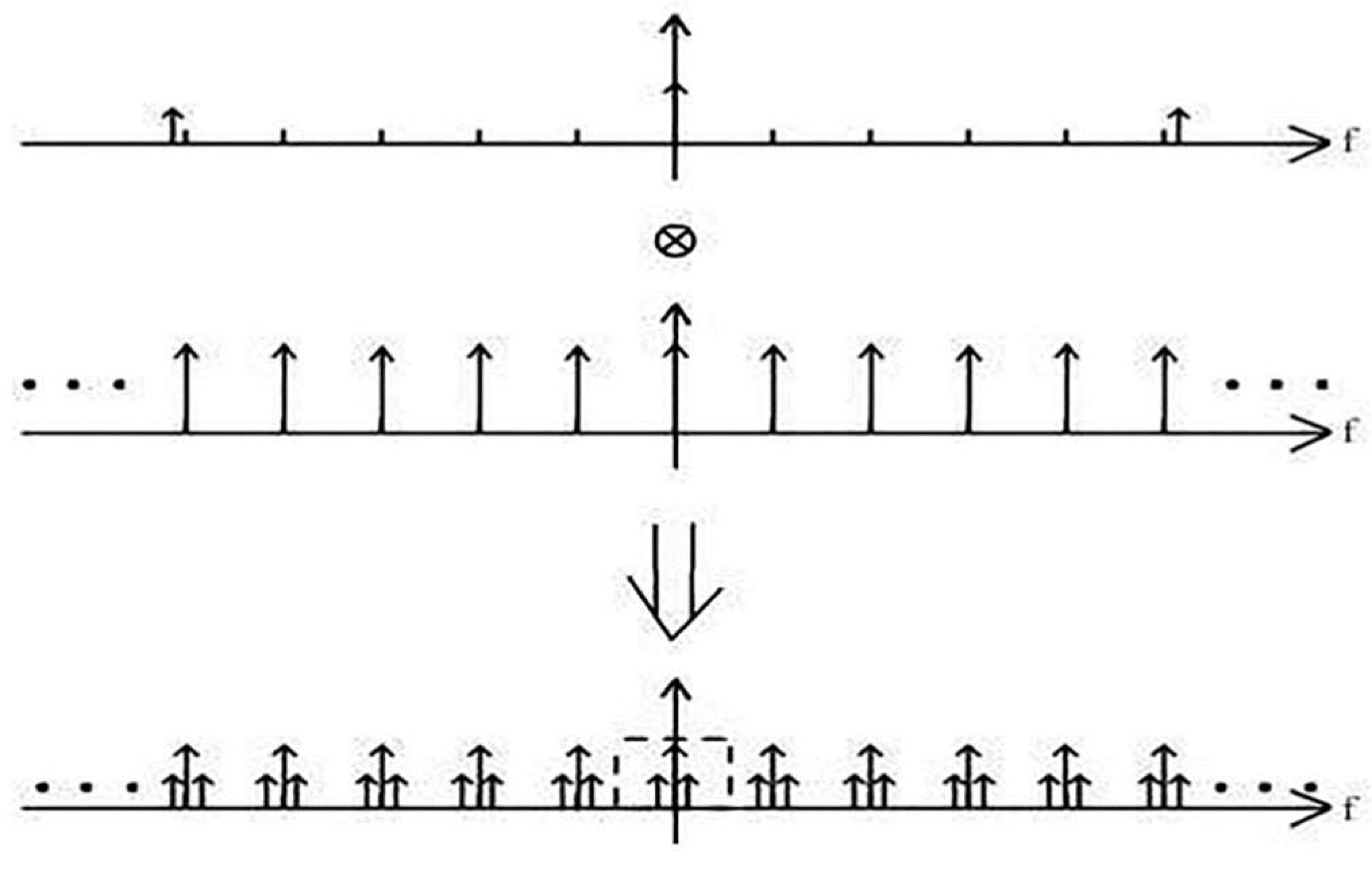
2.3. Wide-Band EMI Imaging

We shifted the high-frequency spectrum to low-frequency spectrum to realize wide-band EMI imaging. Here, optical pulses were used as the electro-optic modulation carrier. Because the down-conversion functions of the optical pulse allow widening of the bandwidth, it improves the sensors’ quality and a narrowband signal processing system measures spatial electric field signal over a large frequency range.

The intensity of the light output by the sensors will vary linearly with the spatial electric field strength within a certain range, thus the output light intensity can be written as follows:

$$I_{out}=\frac{1}{2}{I}_{in}\left(1+\alpha E\right)$$

(1)

Here, I_in is the one-dimensional input light intensity, α is the one-dimensional modulation factor, and E is the added electric field. When an optical signal which carried the spatial electric field information enter a linear photo detector, its output voltage can be expressed as

$$V_{out}=G{I}_{out}=\frac{1}{2}G{I}_{in}\left(1+\alpha E\right)$$

(2)

G is the gain of the sensor. The photo detector converts optical signal into voltage signal. By using the down-conversion characteristics of the pulse light source, the spatial electric field signal at the high frequency can be shifted to the low frequency band, which reduces the bandwidth requirement of the system. The optical signal from the laser has a very narrow pulse width and a very small duty ratio. Its power concentrates on the extremely narrow pulse width. Thus, it is considered as an ideal impulse string as

$$I_{in}=c{\displaystyle \sum }_{n=-\infty }^{+\infty }\delta \left(t-\frac{n}{f_0}\right)$$

(3)

where c is the magnitude of the impulse signal; $\delta (t)$ is the dirac function. When the pulsed light passes through the optical-electric field sensor as described above, the output optical signal can be expressed as:

$$I_{out}=\frac{1}{2}{I}_{in}\left[1+\alpha E\right]=\frac{1}{2}\left[c{\displaystyle \sum }_{n=-\infty }^{+\infty }\delta \left(t-\frac{n}{f_0}\right)\right]$$

(4)

After passing through the sensor, the intensity of the output optical signal contains the input light intensity and the electric field E in Figure 5. The dashed box on the graph represents the photo detector with narrow bandwidth, whose performance likes a low pass filter, which can filter out high frequency components. By using the spectrum shift function of the ideal impulse or low-pass filter, it is possible to transform the electric field signal with a high frequency into a lower frequency voltage.

3. Frequency Identification of EMI Sources

The frequency identification of EMI sources consists of two steps. First, MGRNN block was applied to obtain network weights vectors parameter by training data, and the other MGRNN block which has the determined network parameter weights vectors from the first MGRNN block, was used to the test data to obtain the result of the identification frequency. For MGRNN training: the EMI image dataset was collected and the histogram of the wide-band statistic feature was used to extract feature for network parameter weights training. After that, interference image could be tested by MGRNN, the EMI source would be segmented from the image by multi-threshold segmentation. Feature extraction from the segmented interference sources was used to the MGRNN network to get classification result.

The nodes of the MGRNN hidden layer are represented by the cluster centroids from the modified K-means clustering [20] and the weight vectors parameter at the nodes of the output layer are all set to one, as in the GRNN originally. The frequency identification training and testing process of EMI sources are shown in Figure 6.

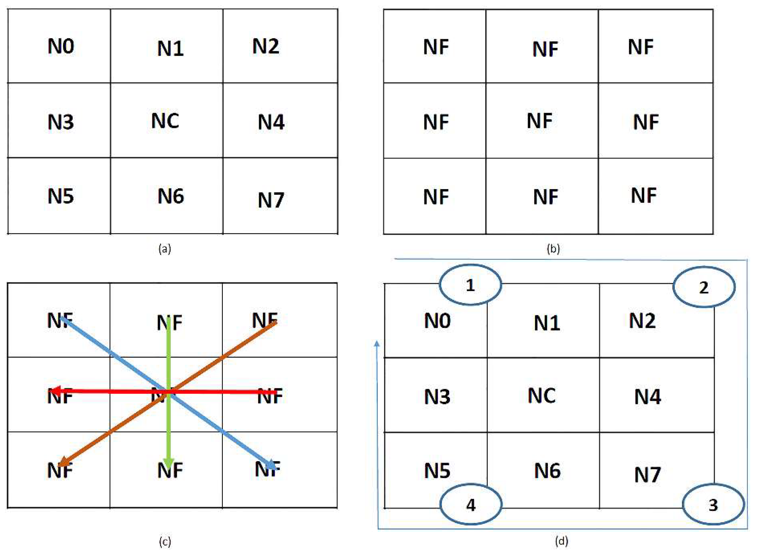
3.1. Multi-Threshold Segmentation

In this paper, we used the maximum entropy method to implement image threshold segmentation. Particle swarm optimization (PSO) was introduced into entropy image segmentation to find the best parameter combination adaptively, as is shown in Figure 7. We applied the proposed peak method to split every interference source from the original image Figure 7a. The processed image Figure 7b was set to threshold value, the other to 0. First, we considered the maximum point of the original image as a center the value NC. Then, we detected the sharp edges of the maximum point signal, and set the threshold values NF accordingly before determining the edge region Figure 7c. Afterwards, we split out the first interference source area in the rectangular area and the set zeros Figure 7d. In the same way, we could split all interference sources and record their maximum position.

3.2. Based on the Histogram of the Wide-Band Statistic Feature

Based on the histogram, we calculated some statistics features which reflect the characteristics of the image [21]: the mean reflects the average gray values of an image; the variance describes the gray value of an image on the numerical discrete distribution. It is a measure of the width of the histogram, which is the difference between the mean and gray level; the skewness means the image histogram distribution asymmetry degree. As the skewness increases, the histogram distribution becomes more asymmetric, otherwise more symmetrical; the kurtosis reflects the general state of an image gray level distribution approach to the mean, the more concentrated; on the contrary, the more dispersion; the energy reflects the uniformity of gray distribution. When energy increases, gray distribution level becomes more homogeneous. The statistical features of the image are used to identify frequency of the interference source.

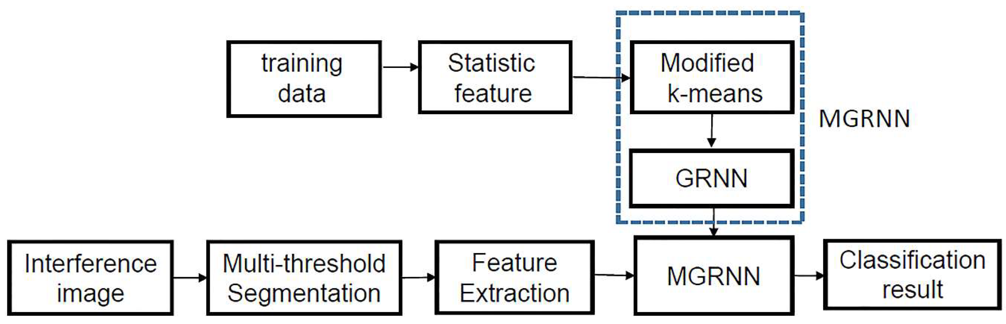
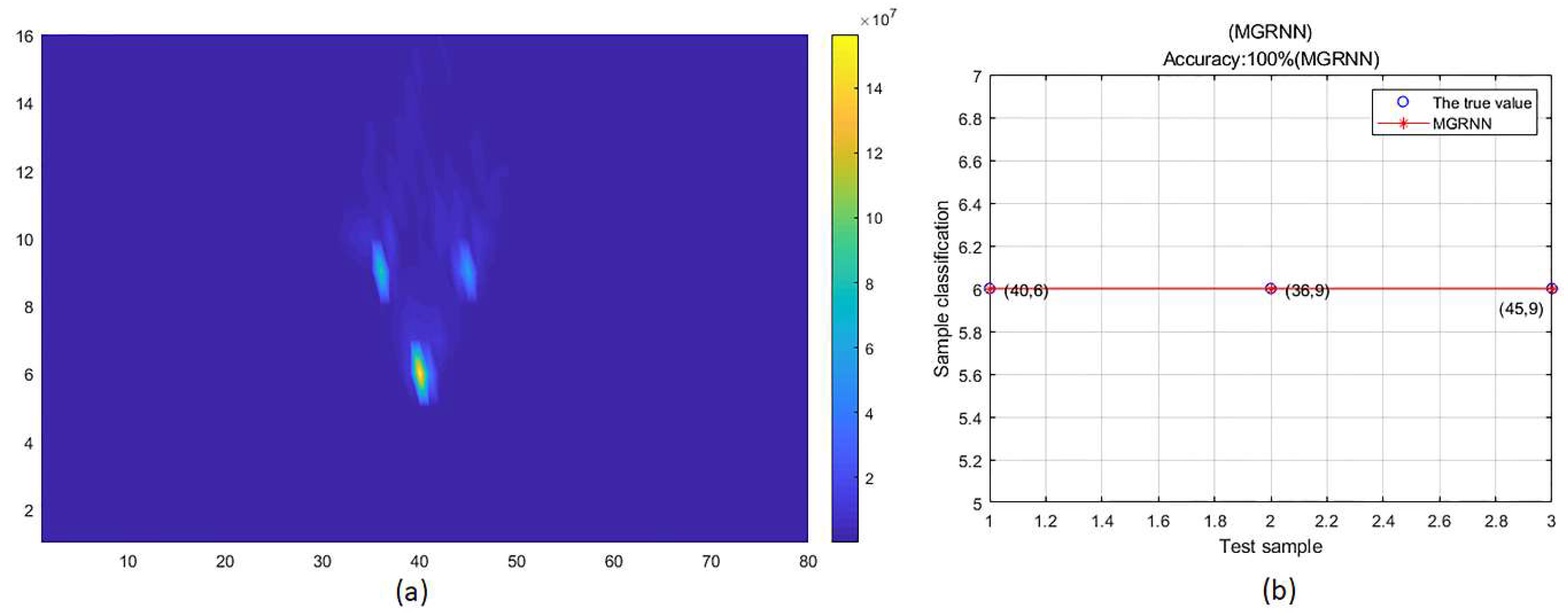
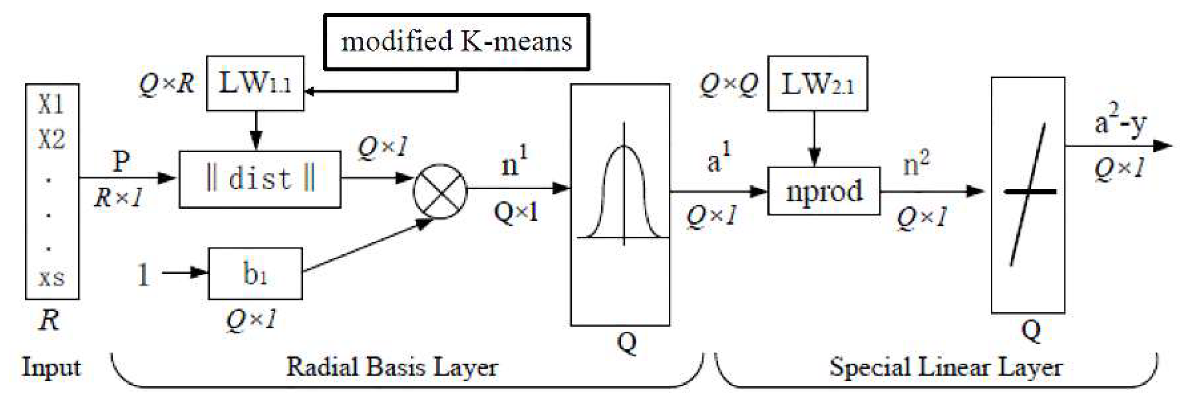
3.3. Modified Generalized Regression Neural Network

A critical consideration in the effectiveness of GRNN is the determination of optimal values for GRNN output weights and input weights. If output weights are fed to the training set outputs, it will give the smallest error when it is used in the final network. If input weights parameter is assigned to all training samples, it is not necessarily the case that this algorithm always presents good predictive accuracy. However, GRNN becomes very large. Obviously, the number of weight parameter is equal to the number of training samples. It is not computationally efficient if the number of training sample is very large. In order to reduce the number of the weight parameters, modified K-means clustering is firstly employed to partition the training data into groups. In each group, the weight parameter is identical for all training samples. The number of multiple weight parameters is then equal to the number of clustering rather than the number of total training set. Therefore, the number of weight parameter is reduced compared to the number of training data.

The modification to GRNN is applied to shrink the hidden layer, and the training data comes from the variance feature of the interference images. Thus, instead of presenting all the variance values of training data samples in the hidden layer nodes for each class, only the means of the resultant clusters are presented. A MGRNN network has the same output layer as GRNN [22]. The structure of MGRNN is shown in Figure 8. P is input; Q is the number of input vectors; b₁ is implicit layer threshold; ‘dist’ is distance function; R is the number of vector elements per group; LW_1.1 is the input layer weight, while LW_2.1 is the weight matrix; n² is output, and a² represents the linear transfer function; nprod is normalized dot product. It has a radial basis layer and a special linear layer.

The radial basis layer can be expressed as

$$a_{1i}=e^{-{(\Vert L{W}_{1.1i}-p\Vert b_{1i})}^2}$$

(5)

where a_1i is the ith element of output a₁, LW_1.1i is the weighted vector made of the ith row of LW_1.1 which is accomplished by performing modified K-means clustering. The second layer is expressed as

$$a^2=purelin(n^2)$$

(6)

where purelin represents linear function as:

$$a=purelin(n)$$

(7)

The training and testing modes of MGRNN are described in the following sections.

MGRNN Training:

(1) Initialize K centre locations using variance feature of the training images.

(2) Cluster points around the centroids, compute corresponding cost C using formula

$$C=\frac{1}{n-n_0}{\displaystyle \sum _i\rho \left(e_i^2\right)}$$

in which

$\rho \left(e_i^2\right)=\{\begin{array}{l}{\Vert x-{\mu }_i\Vert }^2\begin{array}{cc}& \Vert x-{\mu }_i\Vert <T\end{array}\\ 0\begin{array}{c}\Vert x-{\mu }_i\Vert \ge T\end{array}\end{array}$ where $T=3\sigma$ [23].

(3) Update centroids using formula

${\mu }_i^{\left(t+1\right)}=\frac{1}{\left|s_i^{(t)}\right|-\left|s_{io}^{(t)}\right|}{\displaystyle \sum _{x_j\in s_j}{x}_j,x_j=0}$ if $\Vert x-{\mu }_i\Vert >T$ [24], where ${\mu }_i$ is the mean of points in S_j.

(4) Back to (2), until the maximum is reached, or until it stops changing.

(5) Return the partition with minimum C, as a final solution.

(6) The weight vectors of the hidden layer are initialized to the class output clusters.

(7) Set the weight vectors of the output layer as the original GRNN.

MGRNN Testing:

(1) Variance features of input data are presented to the input layer of the network.

(2) The transfer function of the first layer is Formula (5).

(3) Formula (6) is applied to all classes.

(4) Decide which class to classify through the maximum value of the output node.

4. Results and Discussion

We built an imaging system in an anechoic chamber and performed imaging experiments on double-ridged horn antennas (1–18 GHz) in a 5.2 m × 2.6 m rectangular area. The image coordinate origin is the same height as the reflection surface as shown in Figure 9. We used 16 × 1 sensors to scan from the positive direction of the coordinate axis to the negative direction.

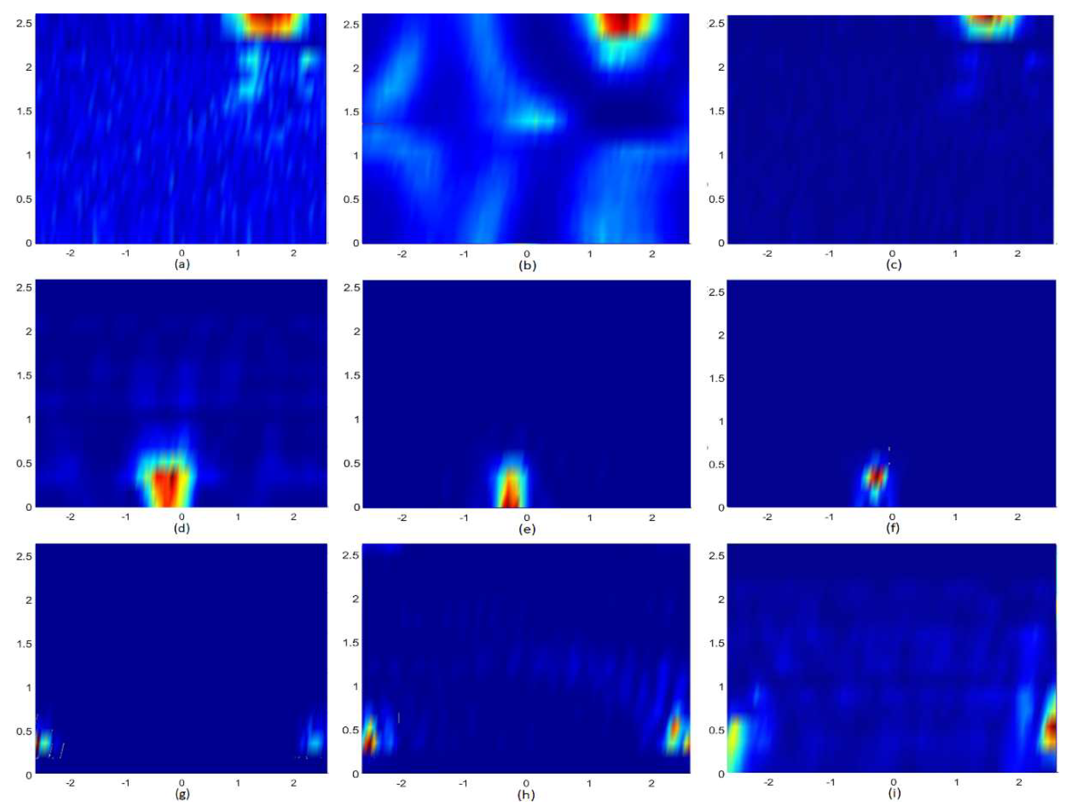
4.1. Localization of Large-Range Wide-Band Electromagnetic Interference Sources

In order to assess the large-range wide-band characteristic of the developed system, horn antennas were placed on the boundary of the object plane, which is in the rectangular area, as shown in Figure 10. The coordinate positions were (−2.6, 0.3) for left, (2.6, 0.3) for right, (1.5, 2.6) for upper and (−0.3, 0) for lower boundary. The input signal power was 15 dBm. The resulting field distribution image reconstructed is shown in Figure 11, with the frequency at 2 GHz, 4 GHz and 6 GHz. As shown in the figures, the resulting field distribution demonstrates that the system was capable of dealing with large-range wide-band circumstances. The position of the radiation source can be accurately obtained and be shown by images.

The position of the double-ridged horn antenna was at −0.3 m and 1.5 m in 2 GHz, 5 GHz and 6 GHz as shown in Figure 12. Input signal power was 15 dBm. As the frequency increased, the signal energy concentrated and the diffraction limitation decreased. The signal maximum value went from −40 dBV to −32 dBV.

We placed a double-ridged horn antenna at (−1 m, 1.5 m) and the source’s movement interval was 30 cm from left to right and from top to bottom. Input signal power was 15 dBm. The position x of each row did not change, and the position y of each column did not change. The electric field values varied as the locations of sources as shown in Figure 13 at 4 GHz and Figure 14 at 6 GHz. Since the symmetrical structure of the reflect surface only verified that it moved from left to right and from top to bottom. The radiation source was close to the origin at the step 30 cm each time, ranging from −40 dBV to −42 dBV at 4 GHz and from −38 dBV to −41 dBV at 6 GHz.

4.2. Multi-Threshold Segmentation Applied on Images

Settings of the experiment were shown as Figure 15a. Three horn antennas were placed (−0.3, 1.2) at 2 GHz, (0.5, 1.3) at 3 GHz and (0.2, 0.3) at 4 GHz as Figure 15b. Under the interference sources of the same frequency at 1 GHz, the original image of the simulation and its segmentation result by the proposed method were shown in Figure 16. Figure 16a was the original image, (b) was the two thresholds segmentation result. Figure 16c showed the three thresholds segmentation result. Figure 17 showed the resulting field distribution of three horn antennas. Figure 16 and Figure 17 were images of different kinds, with quite different characteristics. From Figure 16 and Figure 17, the proposed method obtained satisfactory segmentation results in that these two kinds of images were reasonably divided into objects and background.

When applied to simulation data and experimental data, such an approach can adapt well, because it took the uncertainty of images into account.

4.3. Frequency Identification

The simulation data in Figure 16 and experimental data in Figure 17 using the GRNN for frequency identification were compared with PNN and the radial basis function neural network (RBF), the result was shown in

Table 1. Comparison among PNN, RBF and GRNN.

Method	Variance	Skewness	Kurtosi	Energy
PNN (Figure 16)	95.5%	15.2%	9.3%	41.4%
PNN (Figure 17)	92.3%	14.2%	7.6%	39.7%
RBF (Figure 16)	88%	16%	10%	44%
RBF (Figure 17)	82.4%	14.6%	8.9%	41.1%
GRNN (Figure 16)	98%	16.6%	16%	48%
GRNN (Figure 17)	96.3%	15.2%	12.3%	43.2%

. The average correct-classification-rate of PNN for simulation data and experimental data was 93.9% using the variance feature. For RBF, the average rate was 85.2% and the GRNN was 97.1%. In conclusion, the GRNN performed best using the variance feature compared to other features. Frequency identification was done using the GRNN classifier and the variance feature were chosen for classification reducing dimension of the data.

To verify the result of the modified K-means algorithm using 90 simulation images at different frequencies, we fed 60 images for training and there were 10 images for each classification. 30 images were used as test images and 5 images for each classification. The modified K-means algorithm was closer to the actual point than K-means algorithm in Figure 18, so we can conclude that the modified cluster algorithm which obtained the new centroid of each cluster, can greatly speed up the execution efficiency of clustering analysis algorithm and improve the original k-means accuracy. Applying modified K-means to GRNN (MGRNN) exposed that the average accuracy of the test images was about 96.37%, which is much better than the 91.7% obtained by the developed system with GRNN.

Table 2. Accuracy for classifying interference using MGRNN and GRNN.

Frequency of Interference	MGRNN	GRNN
1 GHz	97.3%	93.1%
2 GHz	96.4%	95.2%
3 GHz	95.5%	91.4%
4 GHz	96.8%	90.1%
5 GHz	95.8%	90.2%
6 GHz	98.3%	90.7%

shows the classification accuracy for interference sources with different frequencies.

Figure 19, Figure 20 and Figure 21 were the simulation images of the multi-frequency multiple interference sources. Our algorithm gave a satisfactory classification result and it had a good adaptability when applied to different kinds of images as the multi-frequency multiple interference sources and the multiple interference sources in same frequency.

5. Conclusions

In this research, a 2D electromagnetic imaging system was applied to localize radiating interference sources and the MGRNN was used to identify the frequency. The experiment proved that MGRNN not only increased accuracy by 5%, which is better than the standard GRNN approaches, but also speed up the process of identification by using modified K-means clustering. In conclusion, the EMI imaging system can realize a large-range wide-band electromagnetic field distribution reconstructed and it provides a new method in the detection capability of electromagnetic interference sources.

References

1. Anastasia, G.; Andrey, B.; Maxim, K.; Yury, K. Localization of cyclostationary EMI sources based on near-field measurements. In Proceedings of the 15th International Conference on Electromagnetics in Advanced Applications (ICEAA), Turin, Italy, 9–13 September 2013; pp. 450–455. [Google Scholar]
2. Oral Salman, A.; Emrullah, B.; Mehmet, S. Textile antenna for the multi-sensor subsurface detection system. In Proceedings of the 13th International Conference on Ground Penetrating Radar (GPR), Castello Carlo VLecce, Italy, 21–25 June 2010. [Google Scholar]
3. Andrey, B.; Anastasia, G.; Maxim, K.; Yury, K. Stochastic EMI sources localization based on ultra wide band near-field measurements. In Proceedings of the 44th European Microwave Conference (EuMC), Rome, Italy, 6–9 October 2014. [Google Scholar]
4. Hui, H.; Pratik, M.; David, P. The development of an EM-field probing system for manual near-field scanning. IEEE Trans. Electr. Comput. 2016, 2, 356–363. [Google Scholar]
5. Hui, H.; Pratik, M.; Andriy, R.; David, P. EM Radiation estimation using an automatic probe position recording system coupled to hand scanning. In Proceedings of the IEEE International Symposium on Electromagnetic Compatibility, Denver, CO, USA, 5–9 August 2013; pp. 349–352. [Google Scholar]
6. Hui, H.; Victor, K.; David, P. 2D Imaging system with optical tracking for EMI source localization. In Proceedings of the IEEE Symposium on Electromagnetic Compatibility and Signal Integrity, Santa Clara, CA, USA, 15–21 March 2015; pp. 107–110. [Google Scholar]
7. Hui, H.; Pratik, M.; David, P. Optical tracking based EM-field probing system for EMC near field manual scanning. In Proceedings of the IEEE International Symposium on Electromagnetic Compatibility (EMC), Raleigh, NC, USA, 4–8 August 2014; pp. 697–701. [Google Scholar]
8. Pratik, M.; Victor, K. Application of emission source microscopy technique to EMI source localization above 5 GHz. In Proceedings of the IEEE International Symposium on Electromagnetic Compatibility (EMC), Raleigh, NC, USA, 4–8 August 2014; pp. 7–10. [Google Scholar]
9. Pratik, M.; Hamed, K.; David, P.; Dikshit, O. Emission source microscopy technique for EMI source Localization. IEEE Trans. Electr. Comput. 2016, 3, 729–736. [Google Scholar]
10. Mojtaba, F.; Joseph, T.; Mohammad, T.G.; Zoughi, R. Piecewise and wiener filter-based SAR techniques for monostatic microwave imaging of layered structures. IEEE Trans. Antennas Propag. 2014, 62, 282–293. [Google Scholar]
11. Liu, Y.; Ravelo, B. Fully time-domain scanning of EM near-field radiated by RF circuits. Prog. Electromagn. Res. (PIER) B 2014, 57, 21–46. [Google Scholar] [CrossRef]
12. Liu, Y.; Ravelo, B.; Jastrzebski, A.K. Time-domain magnetic dipole model of PCB near-field emission. IEEE Trans. Electromagn. Compat. 2016, 58, 1561–1569. [Google Scholar] [CrossRef]
13. Ravelo, B. Radiated near-field emission extraction on 3D curvilinear surfaces from 2D data. Prog. Electromagn. Res. (PIER) M 2015, 44, 191–201. [Google Scholar] [CrossRef]
14. Kaur, R.; Ganju, A. Cloud classification in NOAA AVHRR imageries using spectral and textural features. J. Indian Soc. Remote Sens. 2008, 2, 167–174. [Google Scholar] [CrossRef]
15. Zhang, Y.; Dong, Z.; Wu, L.; Wang, S. A hybrid method for MRI brain image classification. Exp. Syst. Appl. 2011, 38, 10049–10053. [Google Scholar] [CrossRef]
16. Azemi-Sadjadi, M.R.; Gao, W.; Vonder-Haar, T.H.; Reinke, D. Temporal updating scheme for probabilistic neural network with application to satellite cloud classification-further results. IEEE Trans. Neural Netw. 2001, 5, 1196–1203. [Google Scholar] [CrossRef] [PubMed]
17. Specht, D.F. A general regression neural network. IEEE Trans. Neural Netw. 1991, 2, 568–576. [Google Scholar] [CrossRef] [PubMed]
18. Polat, O.; Yildirim, T. Genetic optimization of GRNN for pattern recognition without feature extraction. Expert Syst. Appl. 2007, 4, 25–29. [Google Scholar] [CrossRef]
19. Ning, L.; Yu, C.; Tang, W. GRNN small target detection based on sea clutter. Fire Cont. Radar Technol. 2012, 41, 4–7. [Google Scholar]
20. Zheng, L.G.; Yu, S.J.; Wang, W.; Yu, M.G. Improved prediction of nitrogen oxides using GRNN with K-means clustering and EDA. Fourth Int. Conf. Nat. Comput. 2008, 2, 91–95. [Google Scholar]
21. Liu, Y.X.; Guo, Y.Z. Gray-scale histograms feature extraction using MATLAB. Comput. Knowl. Technol. 2009, 5, 9032–9034. [Google Scholar]
22. Zhu, Z.; Rao, S.H.; Zhang, X.P. Performance prediction of switched reluctance motor using improved generalized regression neural networks for design optimization. CES Trans. Electr. Mach. Syst. 2018, 2, 371–376. [Google Scholar]
23. Rousseeuw, P.J.; Croux, C. Alternatives to the median absolute deviation. J. Am. Stat. Assoc. 1993, 88, 1273–1283. [Google Scholar] [CrossRef]
24. Olukanmi, P.O.; Twala, B. K-means-sharp: Modified centroid update for outlierrobust K-means clustering. In Proceedings of the 2017 Pattern Recognition Association of South Africa and Robotics and Mechatronics (PRASA-RobMech), Bloemfontein, South Africa, 30 November–1 December 2017; p. 17520799. [Google Scholar] [CrossRef]
Figure 1. The electromagnetic imaging system.
Electronics 08 00499 g001
Figure 2. Parabolic reflector.
Electronics 08 00499 g002
Figure 3. The probes. (a) the 16 × 1 probes; (b) the scan path; (c) observation plane.
Electronics 08 00499 g003
Figure 4. The test of the response characteristics of the sensors. (a) the test bench; (b) the response characteristics of the sensors.
Electronics 08 00499 g004
Figure 5. Down-conversion frequency of impulse function.
Electronics 08 00499 g005
Figure 6. Frequency identification training and testing process of EMI sources.
Electronics 08 00499 g006
Figure 7. Image segmentation by PSO. (a) original image value; (b) the threshold image value; (c) make edge region; (d) rectangular area.
Electronics 08 00499 g007
Figure 8. The architecture of MGRNN.
Electronics 08 00499 g008
Figure 9. Settings of the electromagnetic imaging system experiment.
Electronics 08 00499 g009
Figure 10. Settings of the boundary experiment. (a) left and right boundary; (b) upper boundary; (c) lower boundary.
Electronics 08 00499 g010
Figure 11. Boundary imaging. (a) upper boundary of 2 GHz; (b) upper boundary of 4 GHz; (c) upper boundary of 6 GHz; (d) lower boundary of 2 GHz; (e) lower boundary of 4 GHz; (f) lower boundary of 6 GHz; (g) left and right border of 2 GHz; (h) left and right border of 4 GHz; (i) left and right border of 6 GHz.
Electronics 08 00499 g011
Figure 12. The electric field values of the radiation sources at the same location in different frequencies. (a) 2 GHz; (b) 5 GHz; (c) 6 GHz.
Electronics 08 00499 g012
Figure 13. The electric field values vary as the locations of sources at 4 GHz.
Electronics 08 00499 g013
Figure 14. The electric field values vary as the locations of sources at 6 GHz.
Electronics 08 00499 g014
Figure 15. Settings of the segmentation experiment. (a) reflective surface; (b) horn antennas.
Electronics 08 00499 g015
Figure 16. Segmented images of interference sources with same frequency. (a) original image; (b) two thresholds segmentation; (c) three thresholds segmentation.
Electronics 08 00499 g016
Figure 17. Segmented images of interference sources with different frequencies. (a) original image; (b) two thresholds segmentation; (c) three thresholds segmentation.
Electronics 08 00499 g017
Figure 18. Clustering result. (a) K-means clustering; (b) modified K-means clustering.
Electronics 08 00499 g018
Figure 19. Four interference sources with different frequencies at 3 GHz, 3 GHz, 2 GHz and 4 GHz. (a) original image; (b) result of classification.
Electronics 08 00499 g019
Figure 20. Three interference sources with same frequencies at 6 GHz. (a) original image; (b) result of classification.
Electronics 08 00499 g020
Figure 21. Four interference sources with same frequency at 1 GHz. (a) original image; (b) result of classification.
Electronics 08 00499 g021