Review of Pulsed-Eddy-Current Signal Feature-Extraction Methods for Conductive Ferromagnetic Material-Thickness Quantification

Abstract

Thickness quantification of conductive ferromagnetic materials has become a common necessity in present-day structural health monitoring and infrastructure maintenance. Recent research has found Pulsed Eddy Current (PEC) sensing, especially the detector-coil-based PEC sensor architecture, to effectively serve as a nondestructive sensing technique for this purpose. As a result, several methods of varying complexity have been proposed in recent years to extract PEC signal features, against which conductive ferromagnetic material thickness behaves as a function, in return enabling thickness quantification owing to functional behaviours. It can be seen that almost all features specifically proposed in the literature for the purpose of conductive ferromagnetic material-thickness quantification are in some way related to the diffusion time constant of eddy currents. This paper examines the relevant feature-extraction methods through a controlled experiment in which the methods are applied to a single set of experimentally captured PEC signals, and provides a review by discussing the quality of the extractable features, and their functional behaviours for thickness quantification, along with computational time taken for feature extraction. Along with this paper, the set of PEC signals and some MATLAB codes for feature extraction are provided as supplementary materials for interested readers.

1. Introduction

Conductive ferromagnetic wall-like structures are commonly encountered as civil infrastructures, especially in the form of walls of large pipes [1]. Since certain such infrastructures remain underground, and are exposed to factors such as extensive moisture, they often undergo wall loss due to corrosion [2,3]. The quantified remaining wall thickness of such structures becomes an important parameter for their lifetime prediction [3]. This is where thickness quantification of conductive ferromagnetic materials is a necessity in the engineering tasks of structural health monitoring and maintenance.

While several techniques have been investigated for defect and crack detection of conductive materials [4,5,6,7,8,9,10,11,12,13,14,15,16,17,18,19,20], when it comes to thickness quantification of conductive ferromagnetic materials, the Pulsed Eddy Current (PEC) technique, especially the detector coil-based PEC sensor architecture, has been commonly used [21,22,23,24]. The main reason for this associated with detector coil-based PEC sensors can be identified as it being possible to extract signal features that are proportional to the diffusion time constant of eddy currents [23] induced inside a ferromagnetic wall-like structure, and this diffusion time constant behaving as a function of the wall thickness [23]. Consequently, several methods for extracting detector coil-based PEC signal features behaving as functions of thickness have been proposed in recent years [22,24,25,26,27,28]. Some examples for PEC sensing being used for in line inspection of conductive ferromagnetic underground infrastructure are available in References [29,30].

As per recent advancements, related feature-extraction methods targeted towards ferromagnetic material-thickness quantification can be classified into two categories: (1) fitting a sum of exponentials to the signal [22,24] (those references do not provide conclusions about the method); and (2) fitting a straight line to the later stage of the signal [25,26,27,28]. The latter category of line fitting again becomes twofold: (a) least-squares-based fitting [25,26,27]; and (b) Savitzky–Golay filter-based fitting [28]. It is evident that nowadays there is an increased interest towards fast and automated condition assessment of conductive ferromagnetic pipes [29,30], mainly targeted at pipe-wall thickness quantification. PEC sensing has been a leading candidate for available sensing options for the used robotic platforms [29,30]. Therefore, it is important to have a formal analysis of the efficiency of various PEC signal feature-extraction methods for users to decide which algorithms better suit their applications depending on their target robustness levels, the constraints prevalent in the form of required computation speeds, and the available computation power. Motivated by that requirement, this paper contributes by applying PEC signal feature-extraction methods on a set of experimentally captured signals and reviewing the outcomes and implications.

The paper is structured as follows: Section 2 briefly describes the operating principles of the detector coil-based PEC sensor architecture; Section 3 introduces experimentally captured PEC signals used for this work; Section 4 details the procedures for applying the feature-extraction methods found in the literature, and reviews the results they produce along with the complexity of the algorithms; and Section 5 concludes the paper by discussing the implications of results and complexity of the different reviewed feature-extraction methods.

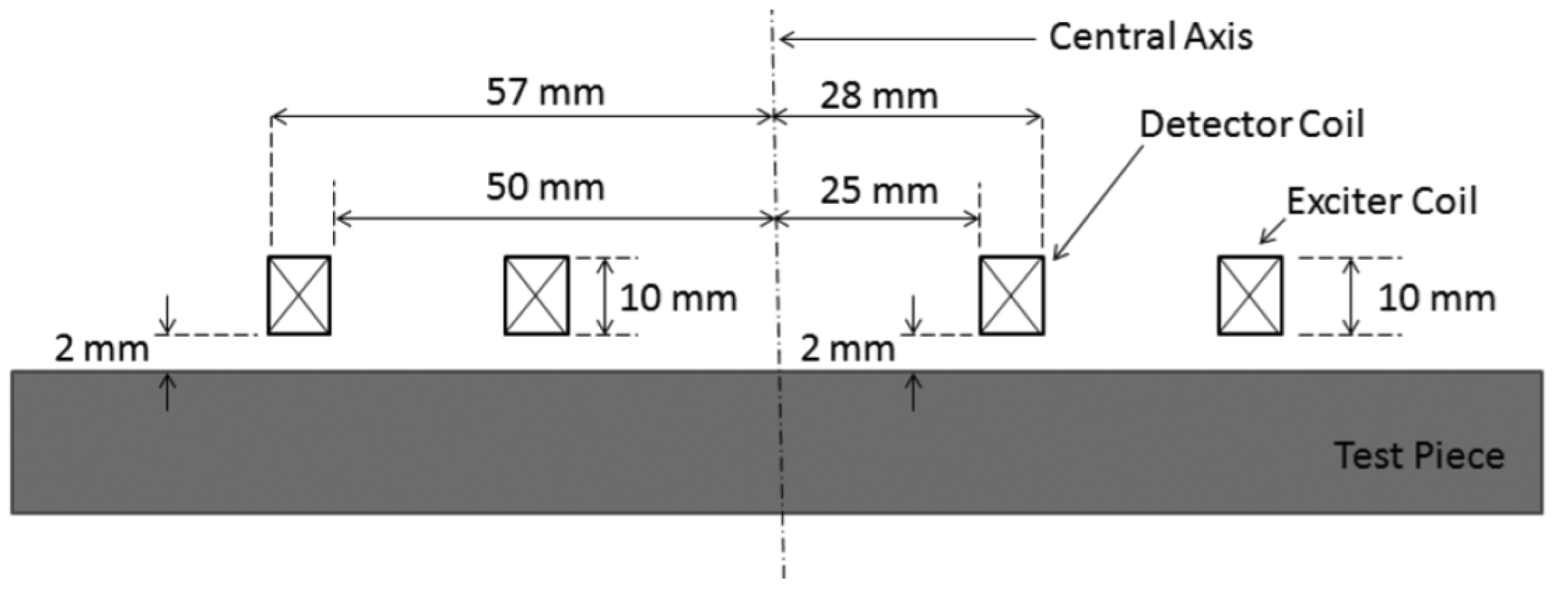
2. Detector Coil-Based PEC Sensors for Ferromagnetic Material-Thickness Quantification: Operating Principles

PEC sensing is a member of the family of Eddy Current (EC) sensing techniques, and Reference [31] is a useful source to read about EC sensing techniques in general. This section briefly describes the operating principles specifically related to detector coil-based PEC sensing.

A detector coil-based PEC sensor architecture is typically composed of two concentrically wound, air-cored, conductive coils [21,22,23,24,25,26,27,28,32,33]. One coil behaves as the exciter, which is excited by a Heaviside step function-like voltage pulse. The excitation causes a rapid change in the surrounding magnetic field, which, in return, induces eddy currents in a conductive test piece placed adjacent to the sensor. The resultant effect of induced eddy currents and the excitation pulse is captured by the second coil, i.e., the detector coil, in the form of a unique time-varying voltage. This detector-coil voltage is identified as the PEC signal that carries information about the test piece. A study [22] has shown this time (t) domain PEC signal, denoted herein as $V\left(t\right)$, can be modelled as an infinite summation of exponential terms, as shown in Equation (1), where for $i\in {\mathbb{Z}}^{+}$, and $b_i$ and $c_i$ are model parameters ($b_i,c_i\in \Re$) containing information about the properties of the sensor and adjacently placed test pieces. Figure 1 shows the typical shape of a detector coil-based PEC signal.

$$V\left(t\right)=\sum _{i=1}^{\infty }{b}_{i}exp(-c_{i}t)$$

(1)

As noted in Reference [23], when a detector coil-based PEC sensor is placed above a uniform, homogeneous, conductive ferromagnetic plate having electrical conductivity $\sigma$, magnetic permeability $\mu$, and thickness d, the dominant time constant $\tau$ of the captured PEC signal, where $\tau \in {\mathbb{R}}^{+},\tau =1/c_j$ for some $j\in {\mathbb{Z}}^{+}$, holds the proportionality $\tau \propto \mu \sigma d^2$. Thus, when $\tau$ is calibrated for a particular material (i.e., $\mu$ and $\sigma$), it becomes a useful signal feature which behaves as a function of thickness d.

A unique attribute of $\tau$, as evident from proportionality $\tau \propto \mu \sigma d^2$, is that $\tau$ is only ‘mainly’ influenced by the thickness and electrical and magnetic properties of the test piece. This in return implies that $\tau$ as a signal feature has a degree of immunity to undesired practical constraints such as lift-off, sensor size, sensor shape, and sensor tilt, which are often encountered in real-world Nondestructive Testing (NDT) and Evaluation (NDE) tasks. This immunity of $\tau$ to such constraints is of great advantage when it comes to real-world NDT and E applications, similar to those reported in References [29,30], and has been studied and published extensively by some previous works [25,26,27].

Based on the model in Equation (1), previous works [22,24,25,26,27,28] all studied extracting signal features to quantify ferromagnetic material thickness, with almost all features having some relationship to the dominant time constant $\tau$. This paper reviews the feature-extraction methods of those works in the sections to come.

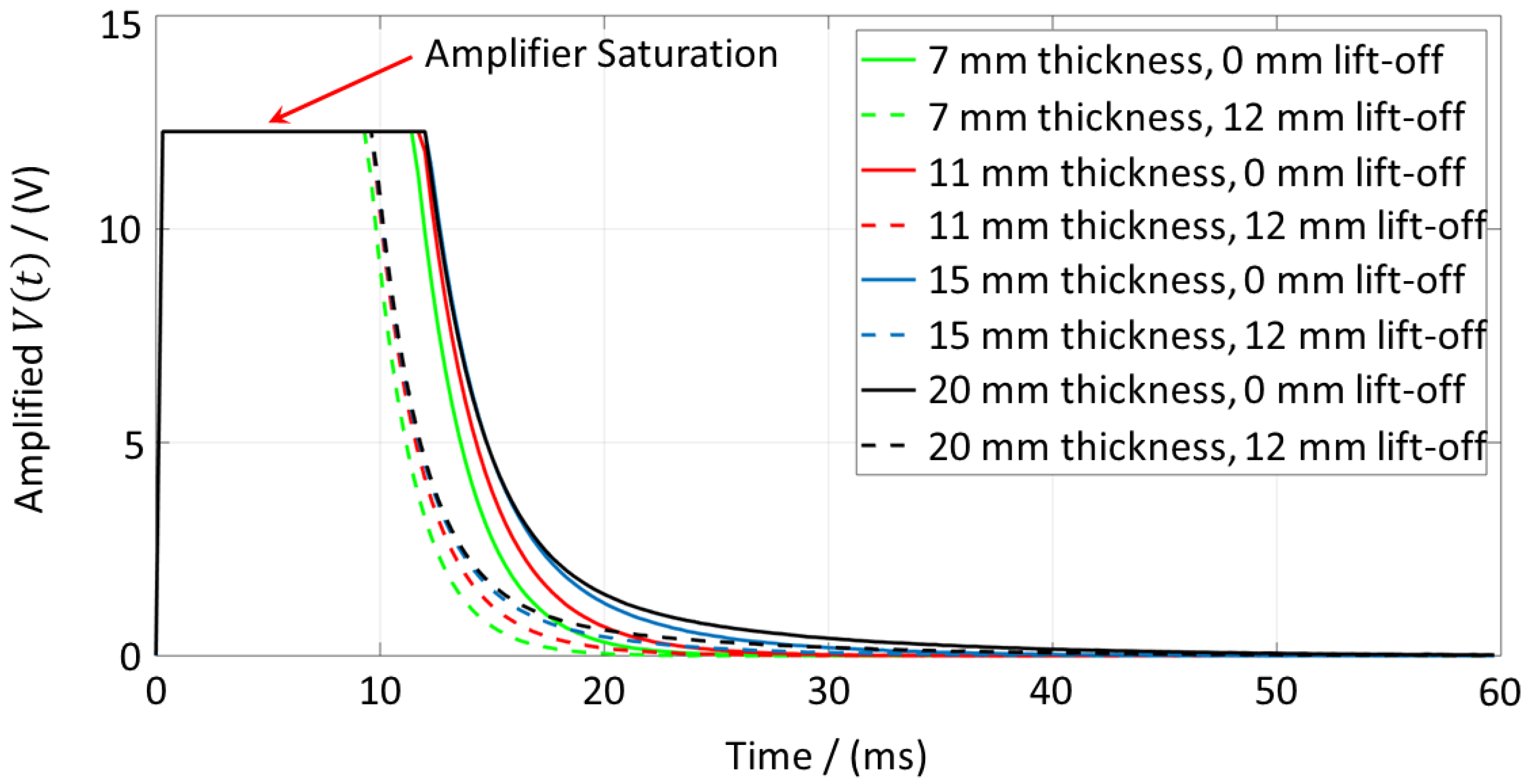
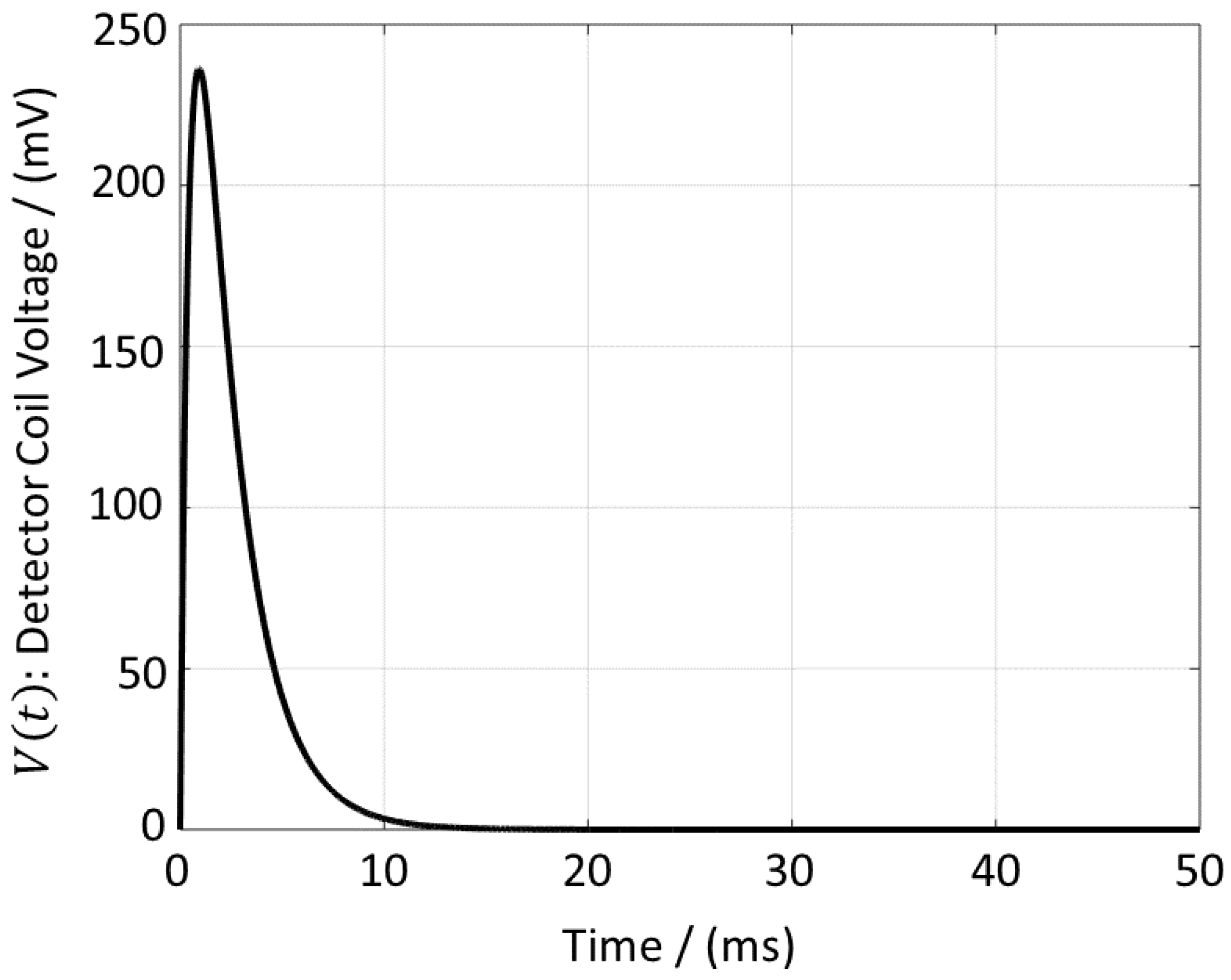
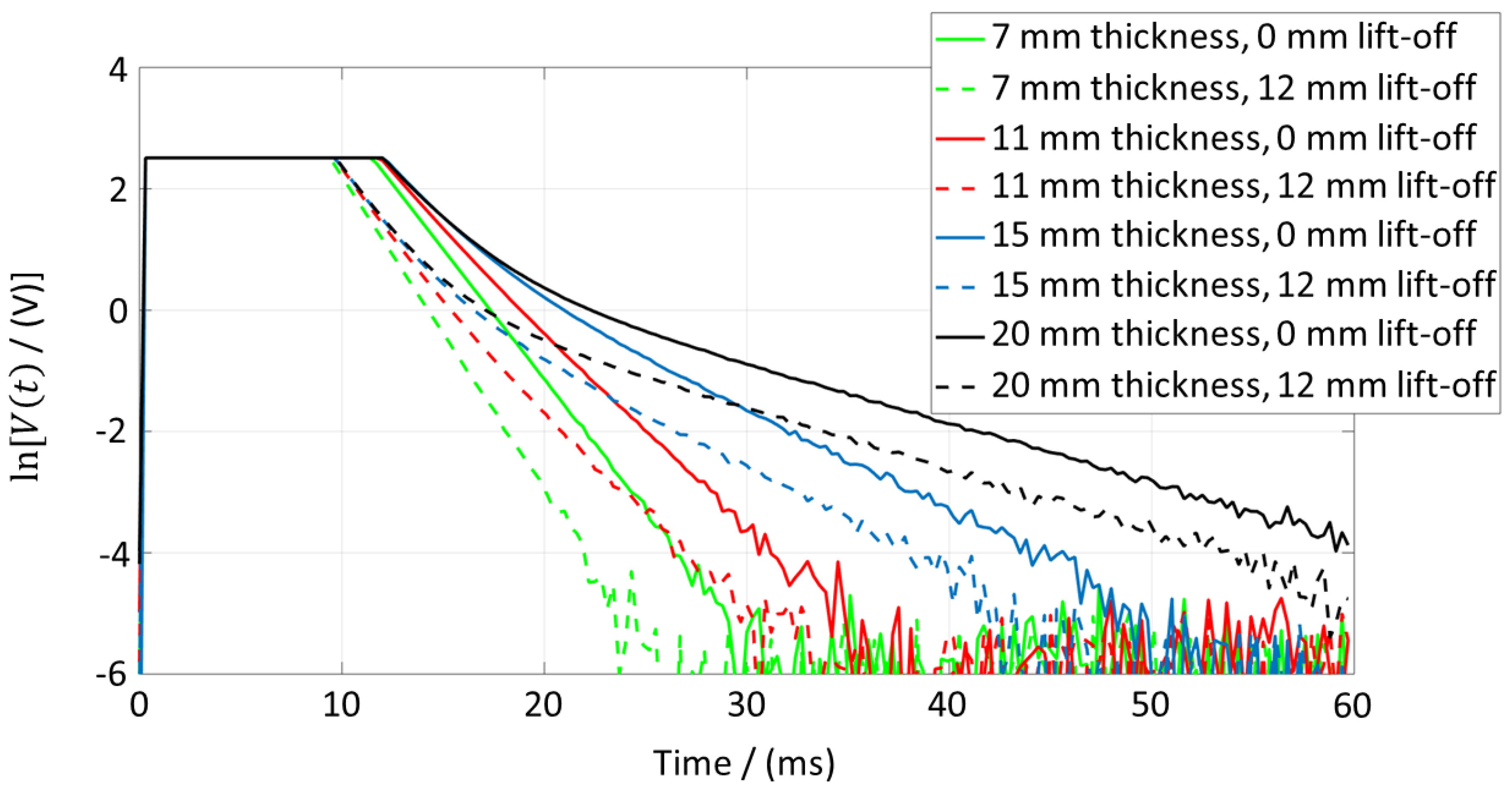
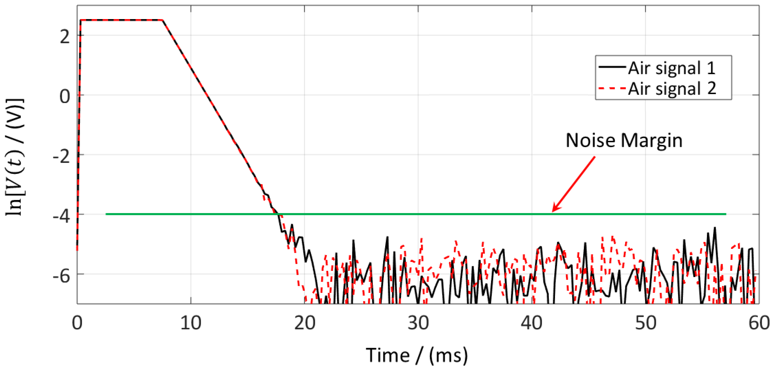
3. Experimental PEC Signals

Experimentally captured PEC signals used in this paper to apply feature-extraction methods were collected on grey cast iron, which is a ferromagnetic material commonly found in aged critical water pipes [34]. Using PEC sensing for condition assessment of grey cast iron is currently of great interest [25,26,27,28,29,30,32,33,34], especially in relation to the task of critical pipe condition assessment [25,26], a real-world NDT application. Signals were captured on grey cast iron blocks of 7, 11, 15, and 20 mm thickness, machined out of a critical pipe test-bed in Sydney Australia. Vintage and location details of the pipe test-bed are provided in Reference [34]. Although the thickness resolution of the blocks is around 4 to 5 mm, it is not indicative of the actual thickness-quantification resolution the sensor can deliver. A formal sensitivity analysis of the sensor related to thickness-quantification resolution has also not been published, but some previous works [25,26,27,29,30,33] showed that the sensor produces thickness estimates that constitute a continuous spectrum.

To examine the impact of lift-off, feature-extraction methods were run on signals captured at two lift-off values (i.e., 0 and 12 mm; 12 mm is an arbitrarily chosen value to be indicative of a moderate lift-off) on the same cast iron blocks. Users can test the feature-extraction methods on any set of signals captured from any detector coil-based PEC sensor. The signals used in this paper were captured from the PEC sensing unit designed and developed by University of Technology Sydney, details of which are published in other works [26,27,32].

Figure 2 shows a cross-sectional image with dimensions of the circular, air cored, concentrically wound PEC sensor used to capture the experimental signals used in this paper. There were 600 exciter-coil turns, and 300 detector-coil turns. The diameter of the copper wire used to wind both coils was 0.315 mm. The sensor was excited with a voltage pulse having 10 V amplitude, 50% duty ratio, and 60 ms pulse width. The induced signals in the detector coil were captured after passing through an instrumentation amplifier of gain 2000. PEC signals used in this paper were generated by averaging curves resulting from 10 consecutive excitation edges (to reduce noise), as done in Reference [24].

The set of signals on which the feature-extraction methods are run in this paper are plotted in Figure 3 and Figure 4. Figure 4 depicts the same signals shown in Figure 3, but in logarithmic scale. The used PEC sensor can capture signals at a sampling interval as low as 15 μs. However, the sampling interval of the signals used to run feature-extraction methods (i.e., the signals plotted in Figure 3 and Figure 4) is 300 μs.

4. Review of Feature-Extraction Methods

Since detector coil-based PEC signals decay with time, as evident in Figure 1 and Figure 3, a signal becomes unusable beyond a certain time due to attenuating below the noise margin of the signal-sampling electronics. Therefore, prior to executing any feature-extraction method, it is important to identify the noise margin in order to select useful signal regions above that margin for processing. The noise margin can easily be visualized by capturing an air signal (i.e., capturing a PEC signal with the sensor placed in air to be indicative of a signal captured in free space) and plotting it in logarithmic scale, as done in Figure 5. One can pick an adequate noise margin by observation; for the signals used in this paper, $ln\left[V\right(t\left)\right]<-4$ (as marked on Figure 5), i.e., $V\left(t\right)<18$ mV was selected as the noise margin. This means that only signal regions greater than 18 mV, i.e., $V\left(t\right)>18$ mV, were used to apply feature-extraction methods in this paper. Some similar techniques to de-noise PEC signals are discussed in Reference [21]. The methods of extracting signal features for thickness quantification are reviewed in the subsections to follow.

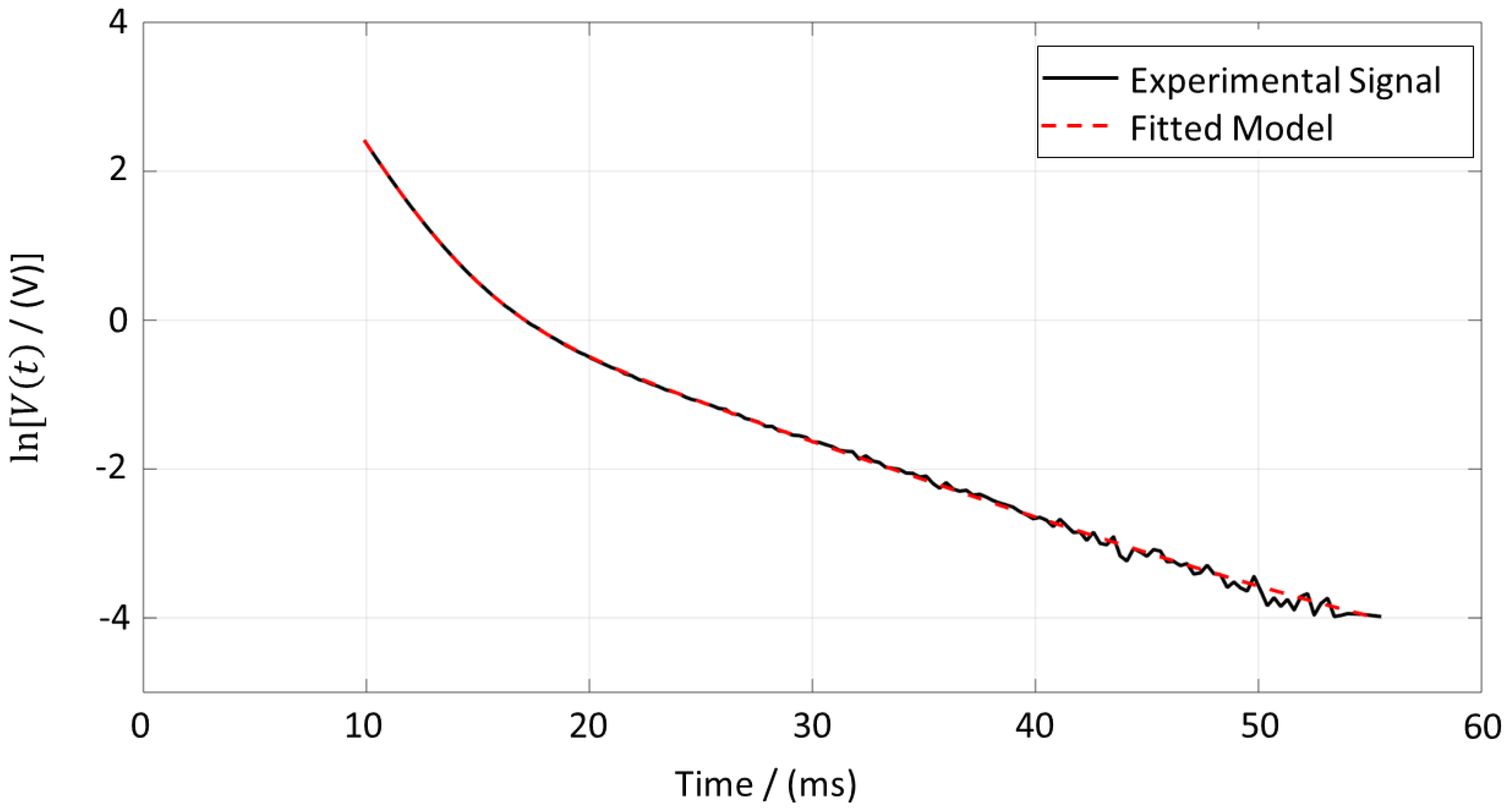
4.1. Fitting a Sum of Exponentials

References related to this method are [22,24]. The idea behind this method is fitting the exponential model presented in Equation (1) to an experimentally captured signal. By doing this, parameter $c_j$, for some $j\in {\mathbb{Z}}^{+}$, corresponding to the dominant time constant, can be estimated, and the reciprocal of this estimated $c_j$ becomes signal feature $\tau$, useful for thickness quantification.

Since the model in Equation (1) is an infinite series, the model as a whole cannot be fitted to a signal. Therefore, the possibility of achieving a satisfactory model fit through fitting a manageable finite number of exponential terms (like two or three) has been examined in [22]. According to that work, three exponential terms seem to provide a reasonable enough fit. However, it is up to the users to decide on how many terms they wish to fit; more terms may be added provided the willingness to bear the cost of complexity.

Following the work in [22], three exponential terms are included in the model used for the work of this subsection; Equation (2) shows the chosen model $V_m\left(t\right)$, where $b_0\in \Re$ characterises small DC offset voltages that can often be present at the output of instrumentation amplifiers [32], which produced the PEC signals used in this work.

$$V_m\left(t\right)=b_0+\sum _{i=1}^3{b}_{i}exp(-c_{i}t)$$

(2)

Fitting a model similar to that in Equation (2) to an experimentally captured signal $V_e\left(t\right)$ similar to those in Figure 3 and Figure 4 can be done through some form of a minimisation of a sum of residuals between the model and the signal. This was done through non-linear least-squares minimisation of the cost function in Equation (3); which means the best fitting parameters (denoted as $param{s}^{*}=[b_0^{*},b_1^{*},c_1^{*},b_2^{*},c_2^{*},b_3^{*},c_3^{*}]$) result as the solution to the optimisation problem presented in Equation (4).

$$cost={\left|\left|V_m\left(t\right)-V_e\left(t\right)\right|\right|}^2$$

(3)

$$param{s}^{*}=\underset{b_0\dots ,b_i,c_i,\dots }{argmin}\left(cost\right)$$

(4)

The work of Reference [22] observed that the minimum $c_i$ value resulting from parameter estimation becomes a signal feature behaving as a function of thickness. Therefore, following parameter estimation, we extracted PEC signal feature $\tau$ as $\tau =1/min(c_1,c_2,c_3)$. The signals and code to solve the above optimisation problem and extract the feature $\tau$ are provided as Supplementary Materials for interested readers to experiment and/or use.

To solve the optimisation, the initial condition set for model parameters was $param{s}_0=[0.01,1,1,1,1,1,1]$. This initial condition was used in common for all signals. Similarly, the common lower and upper boundaries for parameters (denoted as $LB$ and $UB$, respectively) were set to be $LB=[-0.1,0,0,0,0,0,0]$ and $UB=[0.1,{10}^4,{10}^4,{10}^4,{10}^4,{10}^4,{10}^4]$—it is considered as $c_i>0$ $\forall i$ with respect to Equation (2) since the model is fitted only to the decaying part of PEC signals [22,26,27]. Further, optimisation termination criteria used in common for all signals were set to be as follows: Input Tolerance = Output Tolerance = ${10}^{-8}$; and Maximum Function Evaluations = Maximum Iterations = ${10}^4$. Optimisations were solved using the lsqnonlin© solver in MATLAB R2017b^®; the Trust-Region-Reflective algorithm was used.

Since the experimental signals carry a region where the signal reaches amplifier saturation as evident in Figure 3 and the sum of exponentials model does not apply to such saturation regions, the experimental signals $V_e\left(t\right)$ used for fitting were selected such that $V_e\left(t\right)=V\left(t\right)$ where 18 mV $<V\left(t\right)<max\left[V\right(t\left)\right]$; recall the noise margin identified from Figure 5 was 18 mV, i.e., $ln\left[V\right(t\left)\right]\approx -4$. Also note that $max\left[V\right(t\left)\right]$ represents the amplifier saturation voltage (see Figure 3). Figure 6 shows an example for a model fitted to an experimental signal along with the Root Mean Square Error (RMSE) of the fit. The behaviour of thickness against $\tau$ extracted from this method is shown in Section 4.3.

It is noted that the average computing time of this algorithm to extract the signal feature $\tau$ is 413 ms, running on the MATLAB R2017b^® (MathWorks, Natick, MA, USA) platform installed in a Personal Computer (PC) having Intel(R) Core(TM) i7-8550U Central Processing Unit (CPU) @ 1.80∼1.99 GHz with 15.9 GB usable Random Access Memory (RAM).

4.2. Fitting a Straight Line to the Later Stage

Fitting a straight line to the later stage (i.e., as $t>>0$) of the signal is discussed in References [25,26,27,28]. As presented in the works [26,27], this method is based on the PEC signal (when expressed as a logarithm) behaving as a straight line at later stages just before entering the noise margin. This behaviour can be noticed from Figure 4, Figure 5 and Figure 6. Reference [26] expresses this behaviour as:

$$ln\left[V\left(t\right)\right]{|}_{t>>0}\approx -c_{1}t+ln\left[b1\right].$$

(5)

Therefore, if a straight line is fitted to the later stage of a signal and $c_1$ is estimated, required feature $\tau$ used for thickness quantification can be estimated as $\tau =1/c_1$. That, in summary, constitutes the principle behind the methods that fit straight lines to the later stages of PEC signals.

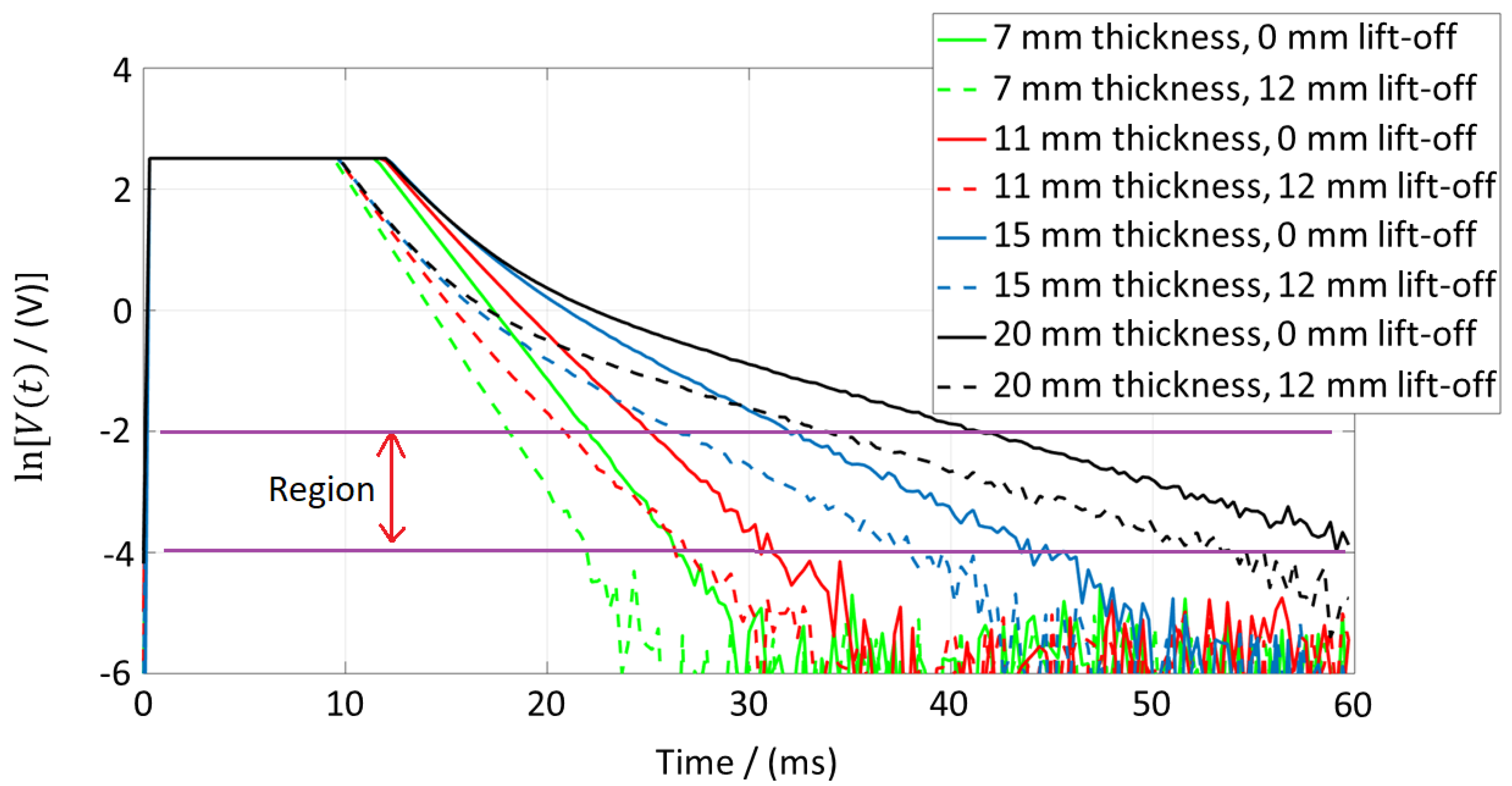
4.2.1. Least Squares-Based Fixed-Region Line-Fitting Method

References [25,26,27] discuss simply extracting $\tau$ by means of linear least squares. First, the signals at hand to be processed are plotted in a logarithmic scale and visualised in order to manually identify a signal region (i.e., a fixed region such that $\alpha <ln\left[V\right(t\left)\right]<\beta$, where $\alpha ,\beta \in \Re$ as $t>>0$) where signals behave approximately as straight lines. An example for a manually identified region, as for the signals in Figure 4, is shown in Figure 7; the identified region is: $-4<ln\left[V\right(t\left)\right]<-2$. Since the range of the linear region has no significance in slope calculation, at times it may be easier to calculate the slope with respect to the X-axis, considering a reference such as the ‘0’ crossing point.

To extract the feature $\tau$, a straight-line model in the form of $y=mt+c$, where y is the dependent variable that represents $ln\left[V\right(t\left)\right]$, t is time, and $m,c\in \Re$ are the gradient and Y-intercept, respectively, is fitted to the identified linear regions of the experimentally captured signals. Then, $\tau$ is obtained as $\tau =1/\left|m\right|$. Figure 8 depicts an example to how a model fitted to a selected linear signal region looks along with the RMSE of the fit. The behaviour of thickness against $\tau$ extracted from this method is shown in Section 4.3.

It is noted that the average computing time of this algorithm to extract signal feature $\tau$ is 2.07 ms, running on the MATLAB R2017b^® (Publisher: MathWorks, Natick, MA, USA) platform installed in a PC with Intel(R) Core(TM) i7-8550U CPU @ 1.80∼1.99 GHz, with 15.9 GB usable RAM.

4.2.2. Savitzky–Golay Filter and Adaptive Least-Squares Fitting-Line (ALSFL)-Based Method

A limitation in the least-squares fitting method discussed in Section 4.2.1 is the region for line fitting being fixed and having to be manually identified through observation. Instead, it is desirable to have the capability to vary the region for line fitting and automatically pick the region within a PEC signal that is best (in some sense), which behaves as a straight line, and extract $\tau$ from that region. Reference [28] proposes a method to achieve this to some extent. In that method, prior to extracting feature $\tau$, Savitzky–Golay filtering [35] is used to experimentally smoothen captured raw PEC signals.

As done in Reference [28], after smoothening PEC signals, in contrast to the method in Section 4.2.1, an ALSFL approach was exploited to search the best fitting line along the smoothened logarithmic PEC signals. Suppose a smoothened PEC signal is $V_s\left(t\right)$; then, first, the sum of logarithms (i.e., $V_{sum}$) is computed as follows:

$$V_{sum}={\int }_{t_1}^{t_2}ln\left[V_s\left(t\right)\right]dt,$$

(6)

where $t_1<t<t_2$ when $t_1,t_2\in \Re$ is the signal duration of interest, such that Noise Margin $<V\left(t\right)<max\left[V\right(t\left)\right]$, as explained in Section 4.1. The intention is to first calculate $V_{sum}$ values from calibration signals acquired on known thickness values (of a particular material) in order to use those values in the form of a look-up table to categorically classify PEC signals acquired on unknown thickness values and prescribe some thresholds for further processing to extract $\tau$. By examining Figure 7, it can be realized how a smaller $V_{sum}$ value corresponds to smaller thickness value, while a larger $V_{sum}$ value corresponds to a relatively larger thickness value, providing the possibility of categorically classifying signals to thickness ranges based on the $V_{sum}$ value. Upon classifying signals, the $V_{sum}$-based look-up table then prescribes a starting point (i.e., a value in $ln\left[V\right(t\left)\right]$ scale) to be used as a starting point for the ALSFL, as well as a region of the signal (known as the ‘search region’) to search for feature $\tau$. Usually, the starting point for lower thickness classes is larger, or higher up in the $ln\left[V\right(t\left)\right]$ scale, while it is lower for higher thickness classes [28]. Starting from the prescribed point, the algorithm fits straight-line models of different lengths, and spans the whole ‘search region’, searching for the best estimate of $\tau$. Model fitting is done using linear least squares in the same way as explained in Section 4.2.1. Fitting is repeated for multiple lengths of the line model, and is stopped when the length reaches a defined maximum length. The mean of absolute distances from relevant samples in the searching sections to their corresponding fitting lines is also calculated, and the fitting line with a minimum mean absolute distance is selected as the best fitting line. Suppose the gradient of the best fitting line is m, then feature $\tau$ is obtained as: $\tau =1/\left|m\right|$. The behaviour of thickness against $\tau$ extracted from this method is shown in Section 4.3 based on the results reported in Reference [28].

An advantage of this method is known to be $\tau$ having better sensitivity to lower thickness values for a given excitation voltage for a given PEC sensor [28]. For a given sensor, a conventional way of having sensitivity to low thickness values is exciting the sensor with lower voltage (this lower voltage is not a precise value, and varies from material to material, as well as the properties of the sensor), and increasing the excitation voltage to have better sensitivity to higher thickness values [26]. However, if one desires to avoid the hardware complexity of having to change the excitation voltage according to thickness values to be estimated, the ALSFL algorithm discussed in this subsection may be advantageous, as it reportedly shows better sensitivity to low thickness values for a given excitation voltage without losing sensitivity to higher thickness values [28].

Based on reported results [28], it is noted that the average computing time of this algorithm to extract signal feature $\tau$ is 14.4 ms, running on the MATLAB R2016a^® platform installed in a PC with Intel Core i5-6500 CPU @ 3.20 GHz.

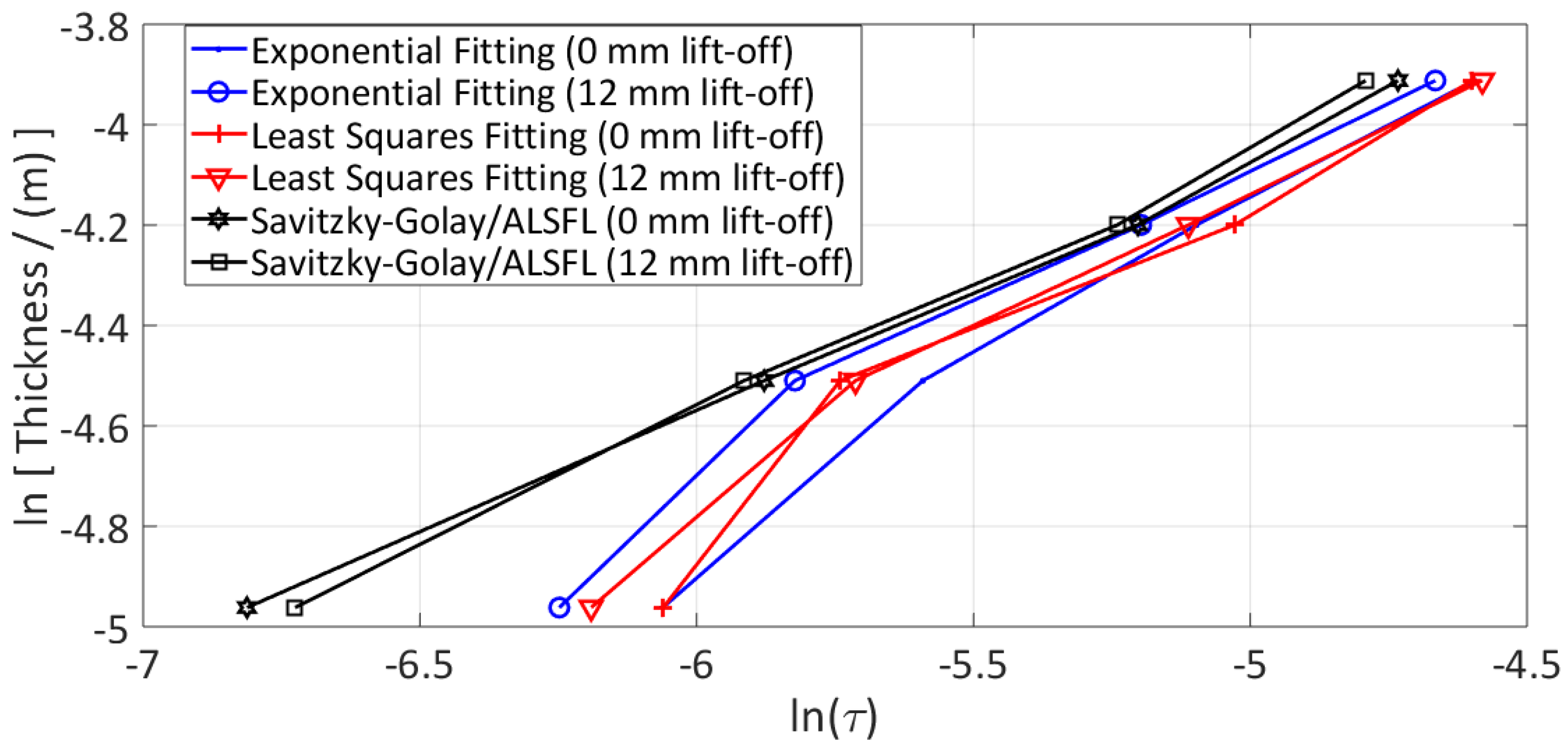
4.3. Results Comparison

Figure 9 shows the functional relationship of thickness against feature $\tau$ extracted through the three methods discussed in Section 4.1, Section 4.2.1 and Section 4.2.2. Following how the functional relationship is visualized in Reference [27], the relationship is plotted in Figure 9 in the form of the thickness logarithm taken in metres against $ln\left(\tau \right)$.

To assess the influence of lift-off on the three methods, the RMSE between $ln\left(\tau \right)$ values resulting from the 0 mm lift-off and the 12 mm lift-off cases for each method was computed. The resulting values were 0.161, 0.0792, and 0.0585 for Exponential Fitting, Least-Squares Fitting, and Savitzky–Golay/ALSFL, respectively. The RMSE values suggest that $\tau$ values estimated from the Savitzky–Golay/ALSFL method were least affected by lift-off, while the $\tau$ values estimated from the Exponential Fitting method were most affected. This suggests that the Savitzky–Golay/ALSFL method could be the better choice on scenarios where high immunity to lift-off is desired. Furthermore, Figure 9 shows how $\tau$ values estimated from the Exponential Fitting and Least Squares methods lose sensitivity as thickness gets lower, while in contrast, the $\tau$ values resulting from the Savitzky–Golay/ALSFL method maintain better sensitivity to lower thickness by maintaining the straight-line-like behaviour between the logarithm of thickness and $ln\left(\tau \right)$. As discussed later in Section 4.2.2, this attribute can be advantageous where one would like to have sensitivity to a larger thickness range (especially including lower thickness values) under a fixed excitation voltage.

Finally, in terms of computation time as calculated in Section 4, the Least Squares method tends to be the fastest (2.07 ms), while the Savitzky–Golay/ALSFL method tends to be the second-fastest (14.4 ms), and, understandably, the Exponential Fitting method tends to be the slowest (413 ms) provided the non-linear optimisation step that has to run within.

5. Conclusions

This paper presented a review of methods used for feature extraction from PEC signals for the purpose of thickness quantification of conductive ferromagnetic materials via NDT and E. The detector-coil-based PEC sensor architecture was specifically in focus. All reviewed methods attempt to extract as a feature, a reasonable representation of what is known as the eddy current diffusion time constant [23] of an inspected test piece. The underlying principle can be summarized as the eddy current diffusion time constant being a parameter predominantly influenced by the electrical and magnetic properties of the test piece, and also thickness; in return, when calibrated for a particular material, this parameter behaving as a function of thickness, and thus enabling thickness quantification if extracted as a signal feature—while showing some reasonable immunity to constraints such as varying lift-off and sensor tilt that often occur in real-world NDT and E tasks.

Three feature-extraction methods were identified and reviewed in this paper, namely: (1) Fitting a Sum of Exponentials, (2) Least Squares-Based Fixed-Region Line-Fitting Method, and (3) Savitzky–Golay Filter and ALSFL-based Method. From the three methods, the Exponential Fitting method seems to have the greatest generality but least practicability when it comes to the requirement of fast, robust, and critical NDT and E applications. The reason for this can be identified as the requirement of having to run some form of a non-linear optimisation step to extract features, and consequently, computation is likely to be time-consuming as well as the results are likely to lack robustness due to some probable subjectiveness to initial and termination conditions provided, and the algorithms used to solve the optimisation (or fitting) problem. However, this method can be very useful for performing extensive analysis on signals at a post-processing stage. In contrast, the line-fitting methods, although lacking in generality when compared with the Exponential Fitting method, seem to be more robust to constraints such as varying lift-off, and faster in terms of computation time.

References

1. Luo, Q.; Shi, Y.; Wang, Z.; Zhang, W.; Li, Y. A Study of Applying Pulsed Remote Field Eddy Current in Ferromagnetic Pipes Testing. Sensors 2017, 17, 1038. [Google Scholar] [CrossRef] [PubMed]
2. Melchers, R.E. Long-term immersion corrosion of steels in seawaters with elevated nutrient concentration. Corros. Sci. 2014, 81, 110–116. [Google Scholar] [CrossRef]
3. Ji, J.; Robert, D.J.; Zhang, C.; Zhang, D.; Kodikara, J. Probabilistic physical modelling of corroded cast iron pipes for lifetime prediction. Struct. Saf. 2017, 64, 62–75. [Google Scholar] [CrossRef]
4. Sophian, A.; Tian, G.Y.; Taylor, D.; Rudlin, J. Design of a pulsed eddy current sensor for detection of defects in aircraft lap-joints. Sens. Actuators A Phys. 2002, 101, 92–98. [Google Scholar] [CrossRef]
5. Sophian, A.; Tian, G.Y.; Taylor, D.; Rudlin, J. A feature extraction technique based on principal component analysis for pulsed eddy current NDT. NDT&E Int. 2003, 36, 37–41. [Google Scholar]
6. Sophian, A. Characterisation of Surface and Sub-Surface Discontinuities in Metals Using Pulsed Eddy Current Sensors. Ph.D. Thesis, University of Huddersfield, Huddersfield, UK, 2003. [Google Scholar]
7. Li, Y.; Jing, H.; Zainal Abidin, I.M.; Yan, B. A Gradient-Field Pulsed Eddy Current Probe for Evaluation of Hidden Material Degradation in Conductive Structures Based on Lift-Off Invariance. Sensors 2017, 17, 943. [Google Scholar] [CrossRef]
8. Li, Y.; Ren, S.; Yan, B.; Zainal Abidin, I.M.; Wang, Y. Imaging of Subsurface Corrosion Using Gradient-Field Pulsed Eddy Current Probes with Uniform Field Excitation. Sensors 2017, 17, 1747. [Google Scholar] [CrossRef] [PubMed]
9. Rifai, D.; Abdalla, A.N.; Razali, R.; Ali, K.; Faraj, M.A. An Eddy Current Testing Platform System for Pipe Defect Inspection Based on an Optimized Eddy Current Technique Probe Design. Sensors 2017, 17, 579. [Google Scholar] [CrossRef]
10. Liu, Z.; Kleiner, Y. State of the art review of inspection technologies for condition assessment of water pipes. Measurement 2013, 46, 1–15. [Google Scholar] [CrossRef]
11. Li, Y.; Wilson, J.; Tian, G.Y. Experiment and simulation study of 3D magnetic field sensing for magnetic flux leakage defect characterisation. NDT&E Int. 2007, 40, 179–184. [Google Scholar]
12. Sophian, A.; Tian, G.Y.; Zairi, S. Pulsed magnetic flux leakage techniques for crack detection and characterisation. Sens. Actuators A Phys. 2006, 125, 186–191. [Google Scholar] [CrossRef]
13. Ivanov, P.A.; Zhang, V.; Yeoh, C.H.; Udpa, H.; Sun, Y.; Udpa, S.S.; Lord, W. Magnetic flux leakage modeling for mechanical damage in transmission pipelines. IEEE Trans. Magn. 1998, 34, 3020–3023. [Google Scholar] [CrossRef]
14. Smith, J.W.K.; Hay, B.R. Magnetic Flux Leakage Inspection Tool for Pipelines. U.S. Patent US6023986A, 15 February 2000. [Google Scholar]
15. Wijerathna, B.; Vidal-Calleja, T.; Kodagoda, S.; Zhang, Q.; Miro, J.V. Multiple defect interpretation based on gaussian processes for mfl technology. SPIE Proc. 2013, 8694, 86941Z. [Google Scholar]
16. Wijerathna, B.; Kodagoda, S.; Miro, J.V.; Dissanayake, G. Iterative coarse to fine approach for interpretation of defect profiles using MFL measurements. In Proceedings of the 10th IEEE Conference on Industrial Electronics and Applications (ICIEA), Auckland, New Zealand, 15–17 June 2015; pp. 1099–1104. [Google Scholar]
17. Kim, D.; Udpa, L.; Udpa, S. Remote field eddy current testing for detection of stress corrosion cracks in gas transmission pipelines. Mater. Lett. 2004, 58, 2102–2104. [Google Scholar] [CrossRef]
18. Xu, X.; Liu, M.; Zhang, Z.; Jia, Y. A novel high sensitivity sensor for remote field eddy current non-destructive testing based on orthogonal magnetic field. Sensors 2014, 14, 24098–24115. [Google Scholar] [CrossRef] [PubMed]
19. Falque, R.; Vidal-Calleja, T.; Miro, J. Defect Detection and Segmentation Framework for Remote Field Eddy Current Sensor Data. Sensors 2017, 17, 2276. [Google Scholar] [CrossRef] [PubMed]
20. Su, D.; Miro, J.V.; Vidal-Calleja, T. Modelling in-pipe acoustic signal propagation for condition assessment of multi-layer water pipelines. In Proceedings of the 10th IEEE Conference on Industrial Electronics and Applications (ICIEA), Auckland, New Zealand, 15–17 June 2015; pp. 545–550. [Google Scholar]
21. Huang, C.; Wu, X.; Xu, Z.; Kang, Y. Pulsed eddy current signal processing method for signal denoising in ferromagnetic plate testing. NDT&E Int. 2010, 43, 648–653. [Google Scholar]
22. Huang, C.; Wu, X.; Xu, Z.; Kang, Y. Ferromagnetic material pulsed eddy current testing signal modeling by equivalent multiple-coil-coupling approach. NDT&E Int. 2011, 44, 163–168. [Google Scholar]
23. Chen, X.; Lei, Y. Excitation current waveform for eddy current testing on the thickness of ferromagnetic plates. NDT&E Int. 2014, 66, 28–33. [Google Scholar]
24. Huang, C.; Wu, X. An improved ferromagnetic material pulsed eddy current testing signal processing method based on numerical cumulative integration. NDT&E Int. 2015, 69, 35–39. [Google Scholar]
25. Ulapane, A.M.N.N.B. Nondestructive Evaluation of Ferromagnetic Critical Water Pipes Using Pulsed Eddy Current Testing. Ph.D. Thesis, University of Technology Sydney, Sydney, Australia, 2016. [Google Scholar]
26. Ulapane, N.; Alempijevic, A.; Vidal-Calleja, T.; Valls Miro, J. Pulsed eddy current sensing for critical pipe condition assessment. Sensors 2017, 17, 2208. [Google Scholar] [CrossRef] [PubMed]
27. Ulapane, N.; Alempijevic, A.; Miro, J.V.; Vidal-Calleja, T. Non-destructive evaluation of ferromagnetic material thickness using Pulsed Eddy Current sensor detector coil voltage decay rate. NDT&E Int. 2018, 100, 108–114. [Google Scholar]
28. Nguyen, L.; Ulapane, N.; Valls Miro, J.; Dissanayake, G.; Munoz, F. Improved Signal Interpretation for Cast Iron Thickness Assessment based on Pulsed Eddy Current Sensing. In Proceedings of the 12th IEEE Conference on Industrial Electronics and Applications, Siem Reap, Cambodia, 18–20 June 2017. [Google Scholar]
29. Miro, J.V.; Hunt, D.; Ulapane, N.; Behrens, M. Towards automatic robotic ndt dense mapping for pipeline integrity inspection. In Field and Service Robotics; Springer: Cham, Switzerland, 2018; pp. 319–333. [Google Scholar]
30. Valls Miro, J.; Ulapane, N.; Shi, L.; Hunt, D.; Behrens, M. Robotic pipeline wall thickness evaluation for dense nondestructive testing inspection. J. Field Robot. 2018, 35, 1293–1310. [Google Scholar] [CrossRef]
31. García-Martín, J.; Gómez-Gil, J.; Vázquez-Sánchez, E. Non-destructive techniques based on eddy current testing. Sensors 2011, 11, 2525–2565. [Google Scholar] [CrossRef] [PubMed]
32. Ulapane, N.; Nguyen, L.; Valls Miro, J.; Alempijevic, A.; Dissanayake, G. Designing A Pulsed Eddy Current Sensing Set-up for Cast Iron Thickness Assessment. In Proceedings of the 12th IEEE Conference on Industrial Electronics and Applications, Siem Reap, Cambodia, 18–20 June 2017. [Google Scholar]
33. Ulapane, N.; Alempijevic, A.; Vidal-Calleja, T.; Miro, J.V.; Rudd, J.; Roubal, M. Gaussian process for interpreting pulsed eddy current signals for ferromagnetic pipe profiling. In Proceedings of the 9th IEEE Conference on Industrial Electronics and Applications, Hangzhou, China, 9–11 June 2014; pp. 1762–1767. [Google Scholar]
34. Miro, J.V.; Rajalingam, J.; Vidal-Calleja, T.; de Bruijn, F.; Wood, R.; Vitanage, D.; Ulapane, N.; Wijerathna, B.; Su, D. A live test-bed for the advancement of condition assessment and failure prediction research on critical pipes. In Proceedings of the Leading-Edge Strategic Asset Management Conference (LESAM13), Sydney, Australia, 9–12 September 2013. [Google Scholar]
35. Schafer, R.W.; Press, W.H.; Teukolsky, S.A. Savitzky-Golay smoothing filters. Comput. Phys. 1990, 4, 669–672. [Google Scholar]
Figure 1. Example for typical shape of a detector coil-based Pulsed Eddy Current (PEC) signal.
Electronics 08 00470 g001
Figure 2. Cross sectional image of the used circular-shaped PEC sensor [27].
Electronics 08 00470 g002
Figure 3. Experimentally captured PEC signals used for the work of this paper.
Electronics 08 00470 g003
Figure 4. Experimentally captured PEC signals used for the work of this paper in logarithmic scale.
Electronics 08 00470 g004
Figure 5. Noise-margin visualization.
Electronics 08 00470 g005
Figure 6. An example model fit, grey cast iron 20 mm thickness and 12 mm lift-off (RMSE = 0.00377).
Electronics 08 00470 g006
Figure 7. Manually picked linear region for straight-line fitting.
Electronics 08 00470 g007
Figure 8. Least-squares line-fitting example, grey cast iron with 20 mm thickness at 12 mm lift-off (RMSE = 0.0762).
Electronics 08 00470 g008
Figure 9. Functional behaviour of thickness against feature τ.
Electronics 08 00470 g009