A PLL-Based Online Estimation of Induction Motor Consumption Without Electrical Measurement


Abstract
:1. Introduction
- conventional energy measurement requires the access to electrical quantities (current, voltage) either as close as possible to the system or in the electrical cabinet where the system is connected;
- the electrical line must feed only the system concerned and not a group consisting of several loads;
- the electrical distribution of the entire site must be perfectly known (electrical drawings are not even available).
- the measuring instruments shall be installed for a period representative of the intended use. Ideally, annual consumption is sought. A measure of consumption over too short a period requires an estimate of the annual operating time in an empirical way, which leads to great uncertainty in the calculation of the annual energy consumption;
- in the case of large sites, the number of motors can be large, which multiplies the measurement points and can increase the cost of the energy audit process in a prohibitive way.
- the running time of the use (T);
- the measurement of the motor speed allowing the electrical power estimation ().
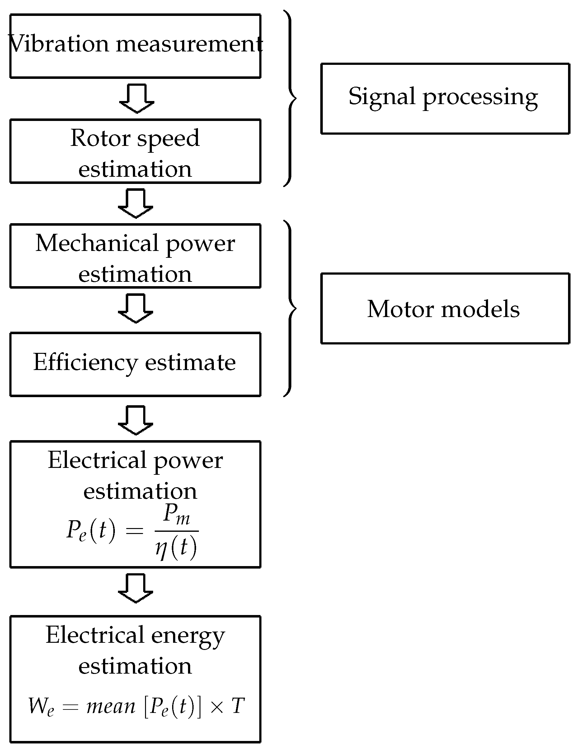
2. Principle of Electrical Power Estimation
2.1. Introduction
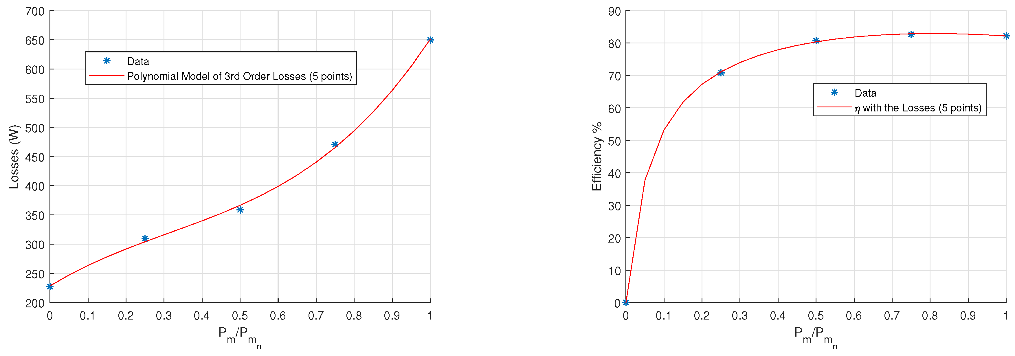
- : mechanical power () as a function of the speed rotational ();
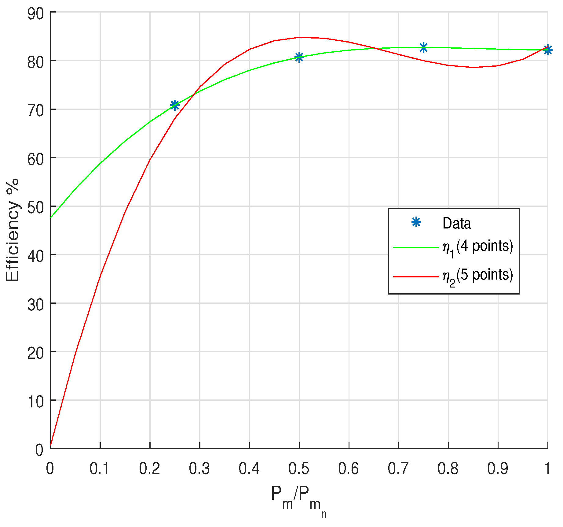
- : efficiency as a function of mechanical power.
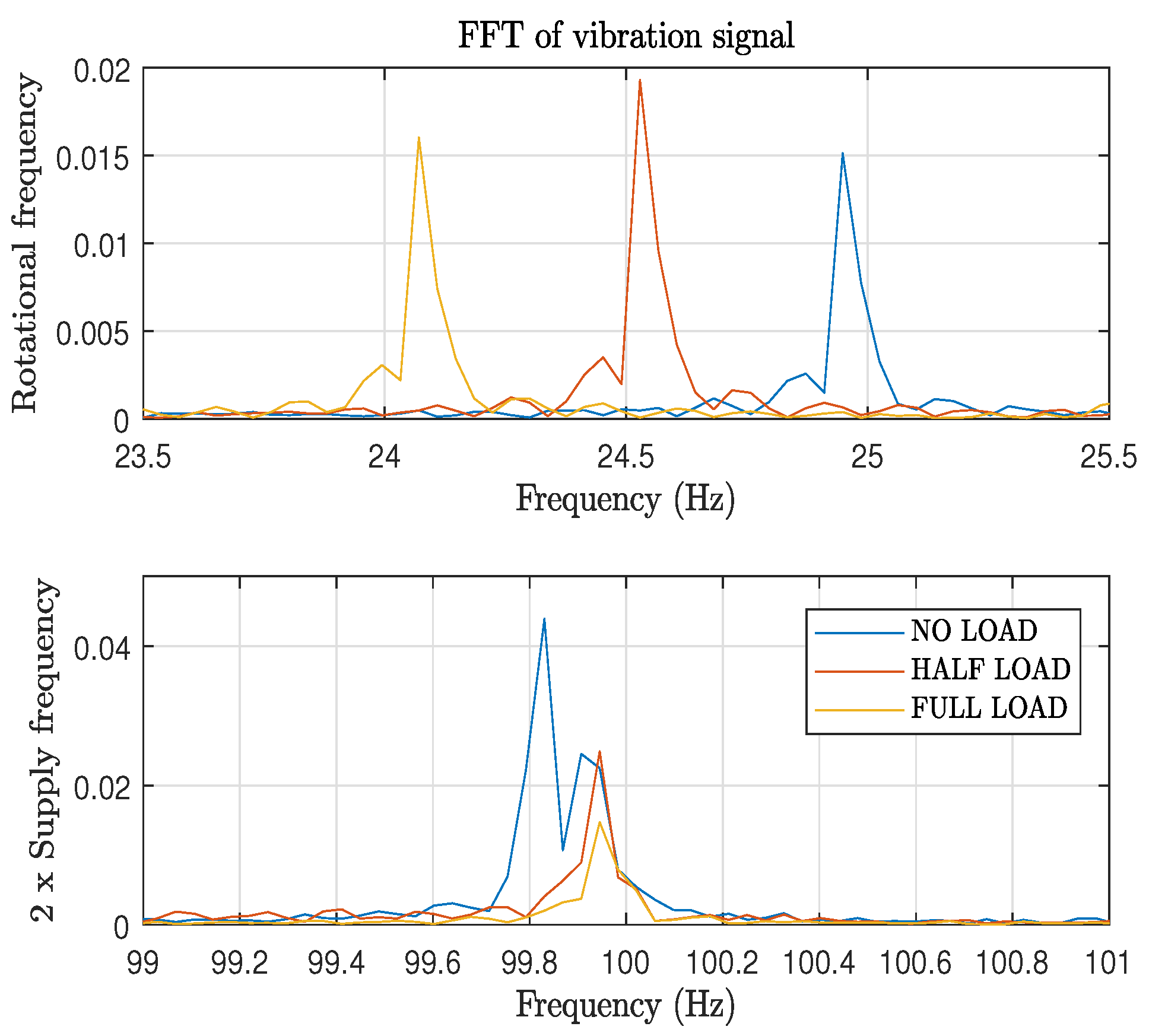
2.2. Vibration Model
- : frequency linked the radial force due to the harmonics of rotor slots.
- : frequency due to the eccentricity of the rotor.
- : frequency due to saturation of the rotor.
- g: constant equal to 0, ±1, ±2...
- : Number of rotor slots.
- : rotation frequency of the rotor.
- : electrical supply frequency.
- : constant equal to 0 or 2.
- : constant equal to 2 or 4.
2.3. Motor Models
2.3.1. Model
2.3.2. Model
2.3.3. Sensibility of Motor Models
3. Online Rotor Speed Estimation
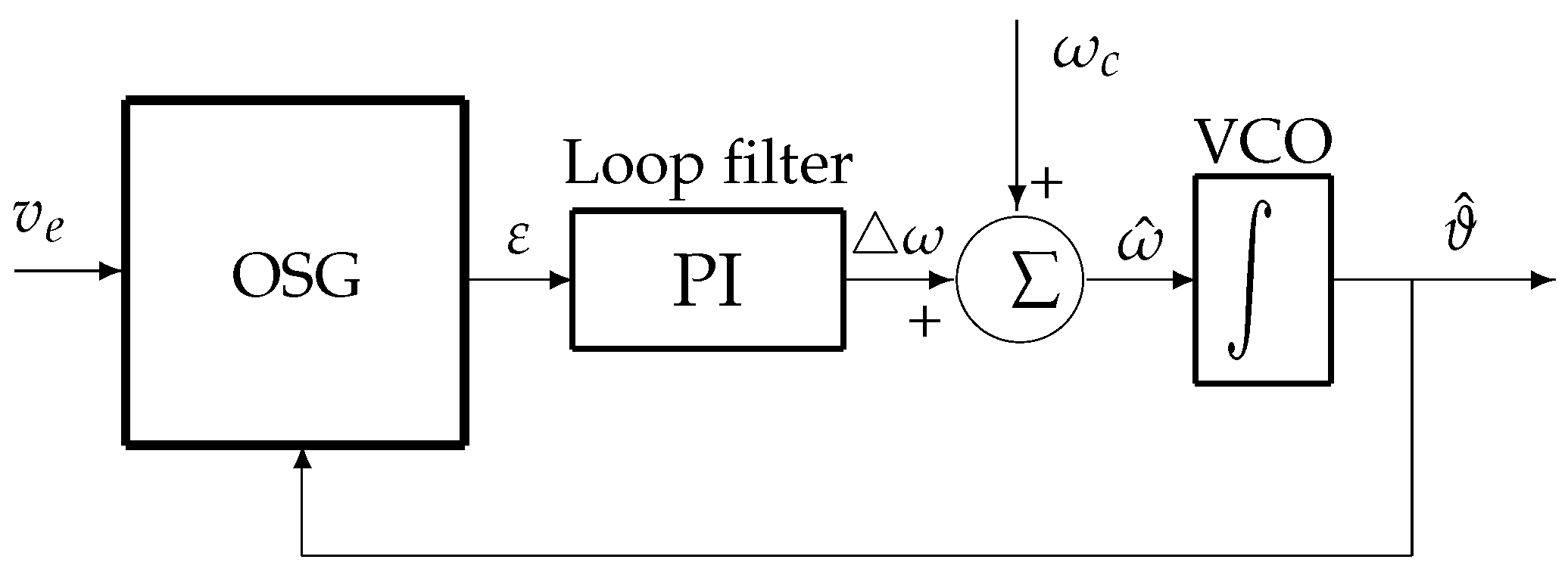
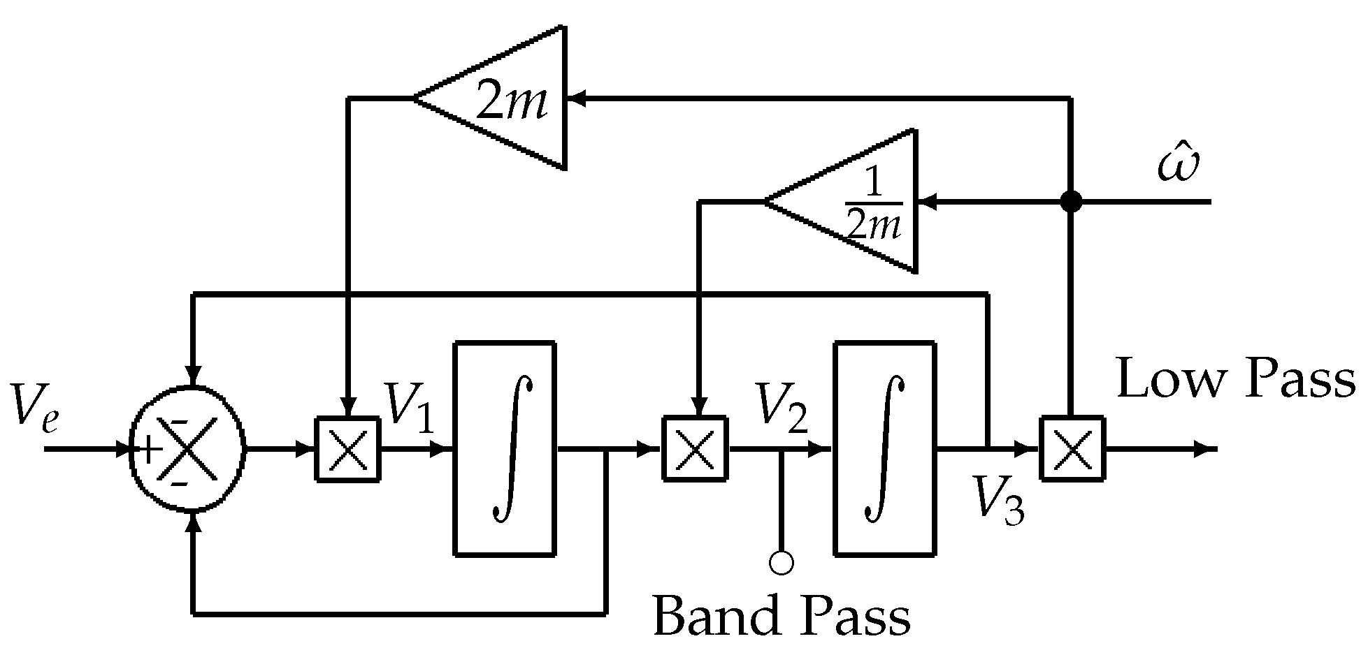
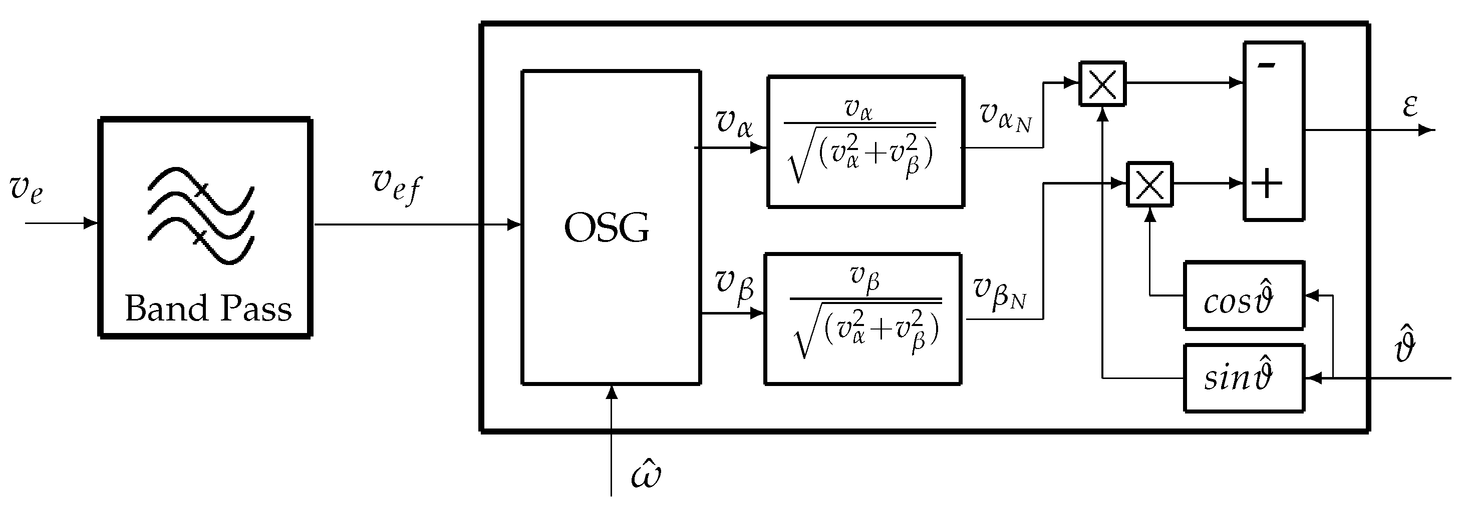
3.1. PLL Principle and Improvements
- : Band-pass filter with a central frequency of ,
- : Low-pass filter with a cut-off frequency of .
- modifying the filter as:
- tuning the two filters with the estimated frequency .
3.2. Simulations
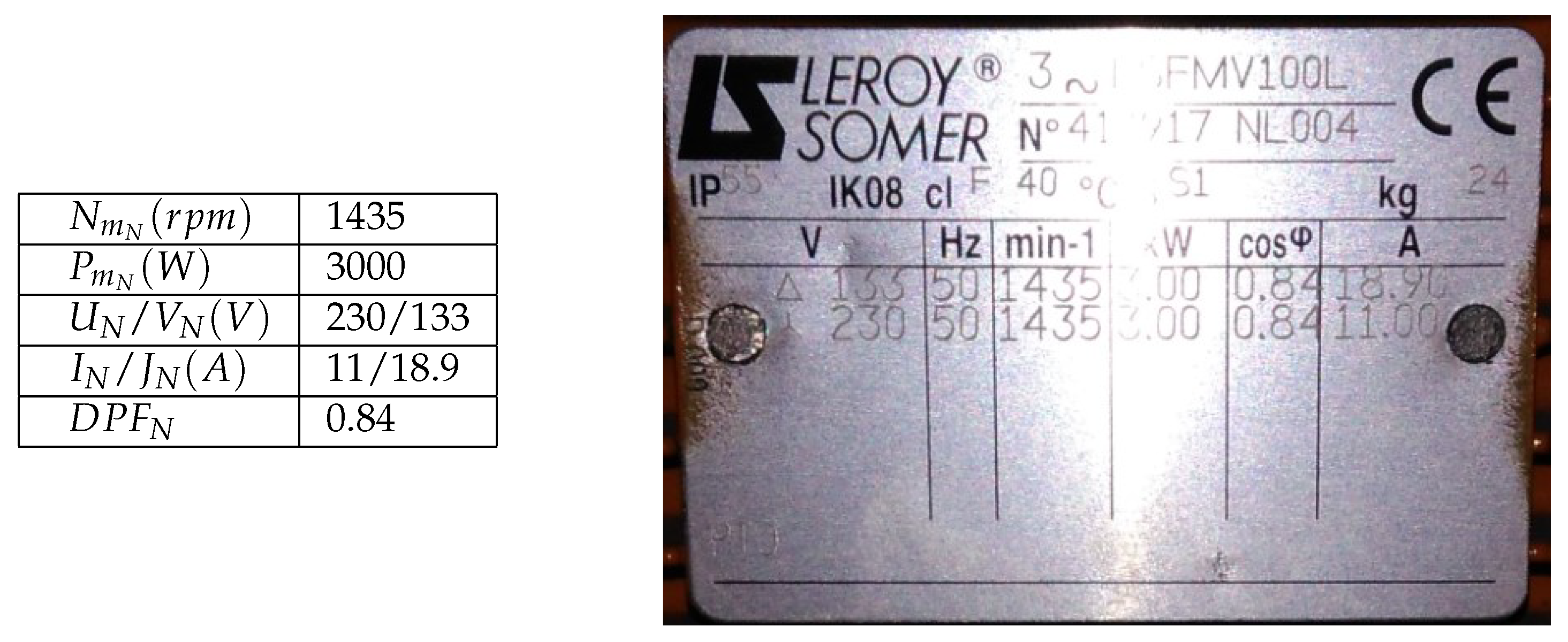
4. Experimental Results
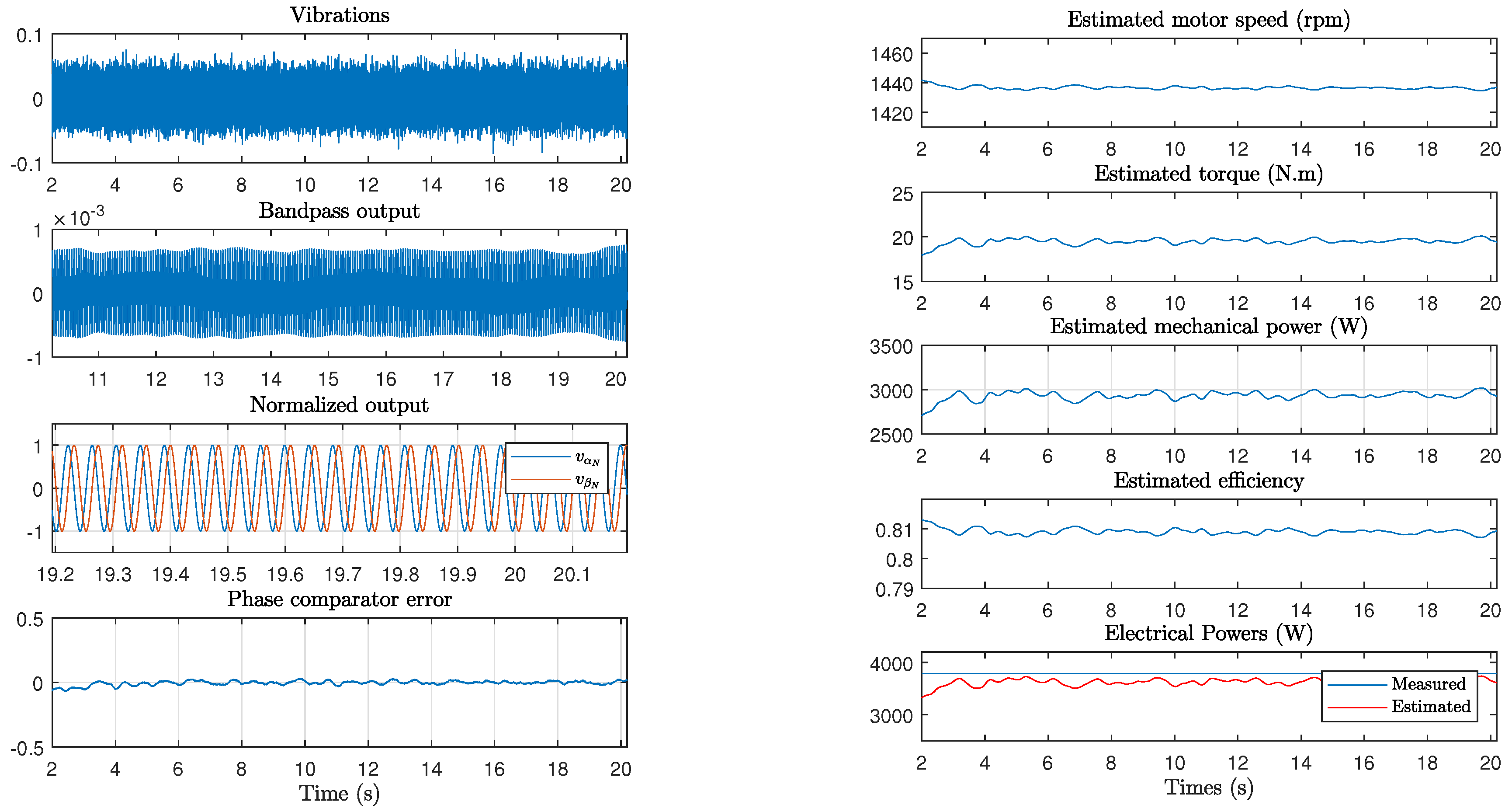
4.1. Constant Speed
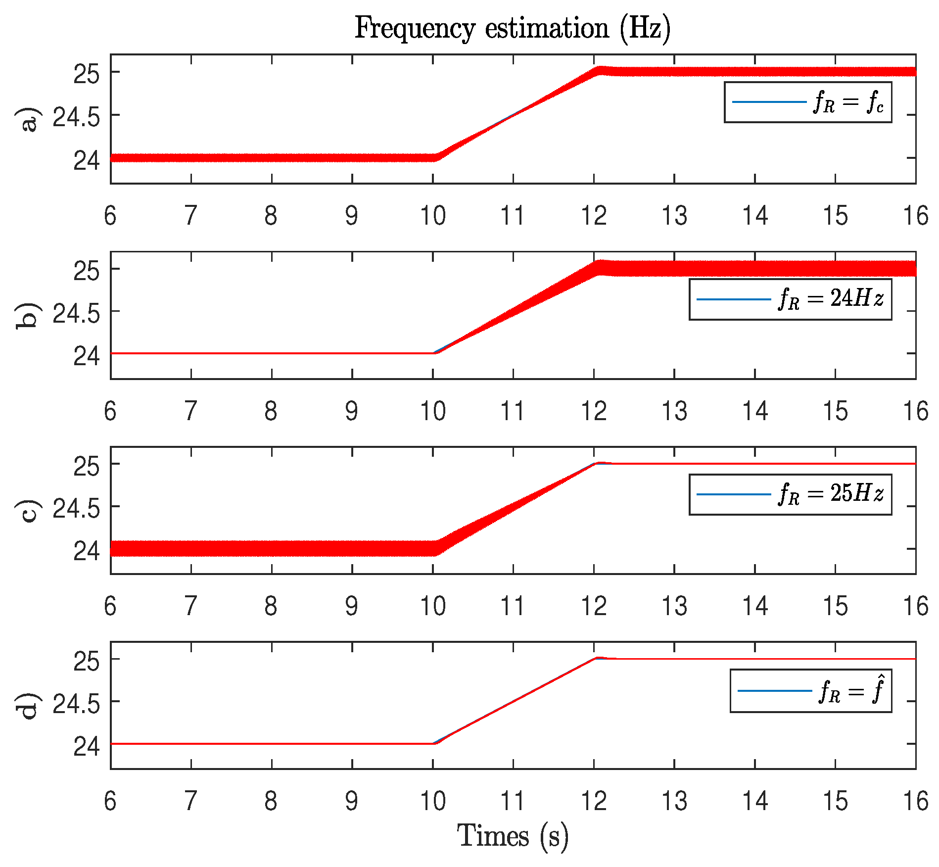
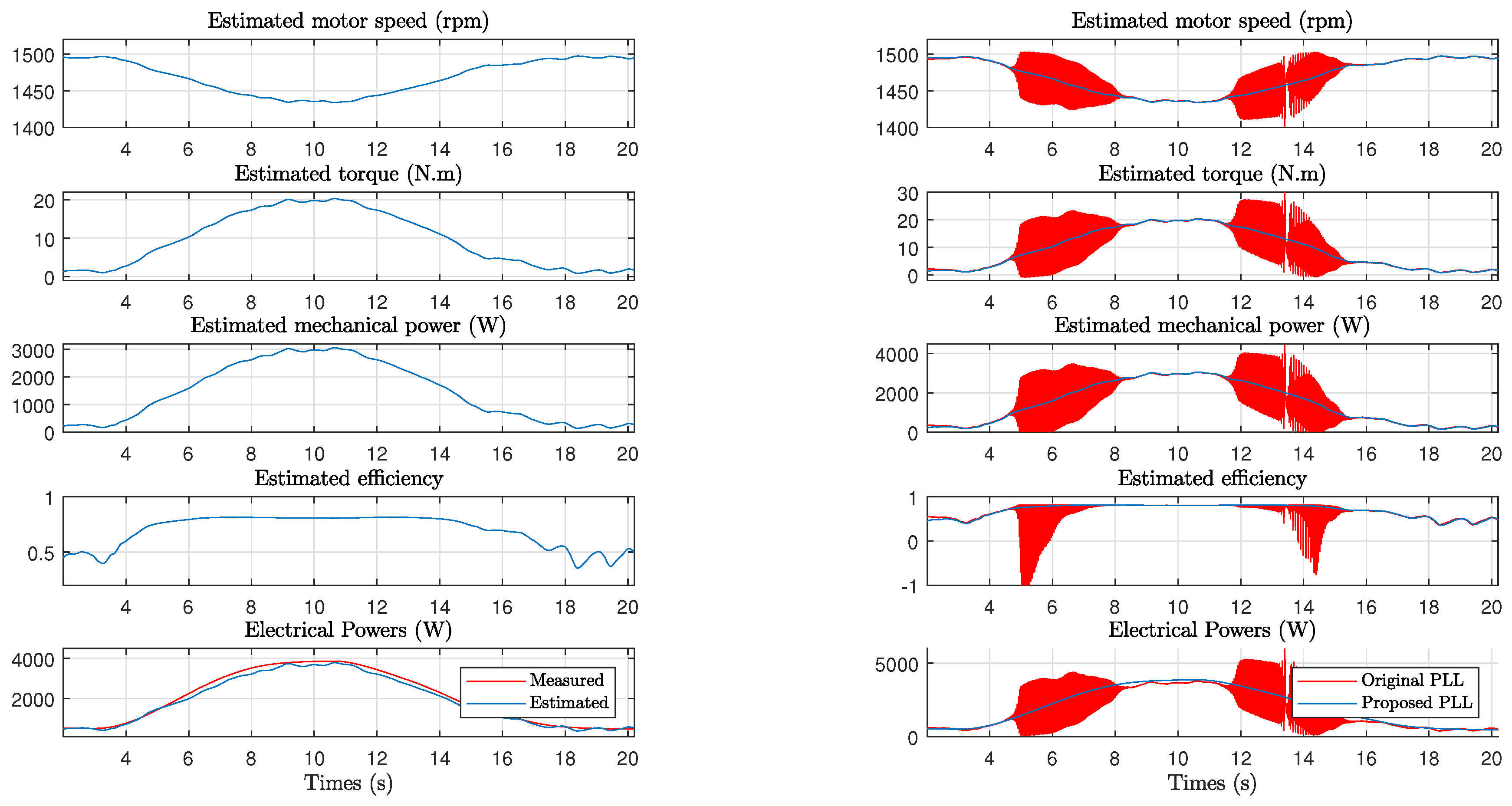
4.2. Variable Speed
- OSG are not tuned with the estimated frequency provided by the PLL,
- OSG at the PLL output is maintained,
- signals are not normalized,
- the P.I the setting is the same as our.
5. Conclusions
Author Contributions
Funding
Acknowledgments
Conflicts of Interest
References
- Zhang, H.; Bradley, K.; Zanchetta, P. A None-Intrusive Load and Efficiency Evaluation Method for In-Service Motors Using Vibration Tests with an Accelerometer. In Proceedings of the IEEE Industry Applications Society Annual Meeting, Edmonton, AB, Canada, 5–9 Octobert 2010. [Google Scholar]
- Dlamini, V.; Naidoo, R.; Manyage, M. A non-intrusive method for estimating motor efficiency using vibration signature analysis. Electr. Power Energy Syst. 2010, 45, 384–390. [Google Scholar] [CrossRef]
- Lin, H.; Ding, K. A new method for measuring engine rotational speed based on the vibration and discrete spectrum correction technique. Measurement 2013, 46, 2056–2064. [Google Scholar] [CrossRef]
- Netsanet, S.; Zhang, J.; Zheng, D. Bagged Decision Trees Based Scheme of Microgrid Protection Using Windowed Fast Fourier and Wavelet Transforms. Electronics 2018, 7, 61. [Google Scholar] [CrossRef]
- Freijedo, F.D.; Doval-Gandoy, J.; Lopez, O.; Fernandez-Comesana, P.; MartinezGions, C. A signal-processing adaptive algorithm for selective current harmonic cancellation in active power filters. IEEE Trans. Ind. Electron. 2009, 56, 2829–2840. [Google Scholar] [CrossRef]
- Golestan, S.; Ramezani, M.; Guerrero, J.M. DQ-frame cascaded delayed signal cancellation-based PLL: Analysis, design, and comparison with moving average filter-based PLL. IEEE Trans. Power Electron. 2015, 30, 1618–1632. [Google Scholar] [CrossRef]
- Yu, B. An Improved Frequency Measurement Method from the Digital PLL Structure for Single-Phase Grid-Connected PV Applications. Electronics 2018, 7, 150. [Google Scholar] [CrossRef]
- Golestan, S.; Monfared, M.; Freijedo, F.D.; Guerrero, J.M. Design and tuning of a modified power-based PLL for single-phase grid-connected power conditioning systems. IEEE Trans. Power Electron. 2012, 27, 3639–3650. [Google Scholar] [CrossRef]
- Thacker, T.; Boroyevich, D.; Burgos, R.; Wang, F. Phase-locked loop noise reduction via phase detector implementation for single-phase systems. IEEE Trans. Ind. Electron. 2011, 58, 2482–2490. [Google Scholar] [CrossRef]
- Han, Y.; Luo, M.; Zhao, X.; Guerrero, J.M.; Xu, L. Comparative Performance Evaluation of Orthogonal-Signal-Generators-Based Single-Phase PLL Algorithms—A Survey. IEEE Trans. Power Electron. 2016, 31, 3932–3944. [Google Scholar] [CrossRef]
- Cao, Y.; Yu, J.; Xu, Y.; Li, Y.; Yu, J. An Efficient Phase-Locked Loop for Distorted Three-Phase Systems. Energies 2017, 10, 280. [Google Scholar] [CrossRef]
- Rodriguez, P.; Teodorescu, P.; Candela, I.; Timbus, A.V.; Liserre, M.; Blaabjerg, F. New positive-sequence voltage detector for grid synchronization of power converters under faulty grid conditions. In Proceedings of the 37th IEEE Annual Power Electronics Specialists Conference, Jeju, Korea, 18–22 June 2006. [Google Scholar]
- Ciobotaru, M.; Teodorescu, R.; Blaabjerg, F. A new single-phase PLL structure based on second order generalized integrator. In Proceedings of the 37th IEEE Annual Power Electronics Specialists Conference, Jeju, Korea, 18–22 June 2006. [Google Scholar]
- Golestan, S.; Monfared, M.; Freijedo, F.D.; Guerrero, J.M. Dynamics assessment of advanced single-phase PLL structures. IEEE Trans. Ind. Electron. 2013, 30, 2167–2177. [Google Scholar] [CrossRef]
- Guan, Q.; Zhang, Y.; Kang, Y.; Guerrero, Y.M. Single-Phase Phase-Locked Loop Based on Derivative Elements. IEEE Trans. Power Electron. 2016, 32, 4411–4420. [Google Scholar] [CrossRef]
- Boglietti, A.; Cavagnino, A.; Lazzari, M.; Pastorelli, M. International Standards for the Induction Motor Efficiency Evaluation: A Critical Analysis of the Stray-Load Loss Determination. IEEE Trans. Ind. Appl. 2004, 40, 1294–1301. [Google Scholar] [CrossRef]
- Lu, B.; Habetler, T.G.; Harley, R.G. A survey of efficiency-estimation methods for in-service induction motors. IEEE Trans. Ind. Appl. 2006, 42, 924–933. [Google Scholar]
- Al-Badri, M.; Pillay, P.; Angers, P. A Novel In Situ Efficiency Estimation Algorithm for Three-Phase IM Using GA IEEE Method F1 Calculations and Pretested Motor Data. IEEE Trans. Energy Convers. 2015, 30, 1092–1102. [Google Scholar] [CrossRef]
- Salomon, C.P.; Santana, W.C.; Lambert-Torres, G.; Borges da Silva, L.; Bonaldi, E.; de Oliveira, L. Comparison among Methods for Induction Motor Low-Intrusive Efficiency Evaluation Including a New AGT Approach with a Modified Stator Resistance. Energies 2018, 11, 691. [Google Scholar] [CrossRef]
- Wu, D.; Pekarek, S.D. Using Mechanical Vibration to Estimate Rotor Speed in Induction Motor Drives. In Proceedings of the 2007 IEEE Power Electronics Specialists Conference, Orlando, FL, USA, 17–21 June 2007. [Google Scholar]
- Al-Jufout, S.A.; Al-rousan, W.H.; Wang, C. Optimization of Induction Motor Equivalent Circuit Parameter Estimation Based on Manufacturer’s Data. Energies 2018, 11, 1792. [Google Scholar] [CrossRef]
- Szychta, L.; Figura, R. Analysis of efficiency characteristics of squirrel-cage induction motor for pump applications. In Proceedings of the 2012 International Conference on Electrical Machines, Marseille, France, 2–5 September 2012. [Google Scholar]
- Gardner, F.M. Phase Lock Techniques; Wiley: New York, NY, USA, 1979. [Google Scholar]


| 0 | |||||
| (Hz) | D (s) | ||
|---|---|---|---|
| 10 | ≈30 | ≈0.3 | >3 |
| 5 | ≈20 | ≈0.2 | >5 |
| 1 | ≈4 | ≈0.04 | >25 |
| No Load | Half Load | Full Load | |
|---|---|---|---|
| (rpm) | 1496.7 | 1464.6 | 1435.5 |
| (rpm) | 1497.1 | 1464.1 | 1436.4 |
| (%) | 0.0272 | 0.0404 | 0.064 |
| (N.m) | 0.893 | 11.04 | 19.53 |
| (W) | 140 | 1692.7 | 2938.4 |
| (%) | 35.1 | 80 | 80.89 |
| (W) | 392.77 | 2115.6 | 3623.3 |
| (W) | 375.46 | 2319 | 3785.3 |
| (%) | 4.61 | 8.8 | 4 |
© 2019 by the authors. Licensee MDPI, Basel, Switzerland. This article is an open access article distributed under the terms and conditions of the Creative Commons Attribution (CC BY) license (http://creativecommons.org/licenses/by/4.0/).
Share and Cite
Doget, T.; Etien, E.; Rambault, L.; Cauet, S. A PLL-Based Online Estimation of Induction Motor Consumption Without Electrical Measurement. Electronics 2019, 8, 469. https://doi.org/10.3390/electronics8040469
Doget T, Etien E, Rambault L, Cauet S. A PLL-Based Online Estimation of Induction Motor Consumption Without Electrical Measurement. Electronics. 2019; 8(4):469. https://doi.org/10.3390/electronics8040469
Chicago/Turabian StyleDoget, Thierry, Erik Etien, Laurent Rambault, and Sébastien Cauet. 2019. "A PLL-Based Online Estimation of Induction Motor Consumption Without Electrical Measurement" Electronics 8, no. 4: 469. https://doi.org/10.3390/electronics8040469
APA StyleDoget, T., Etien, E., Rambault, L., & Cauet, S. (2019). A PLL-Based Online Estimation of Induction Motor Consumption Without Electrical Measurement. Electronics, 8(4), 469. https://doi.org/10.3390/electronics8040469