A Novel Arc Fault Detection Method Integrated Random Forest, Improved Multi-scale Permutation Entropy and Wavelet Packet Transform


Abstract
:1. Introduction
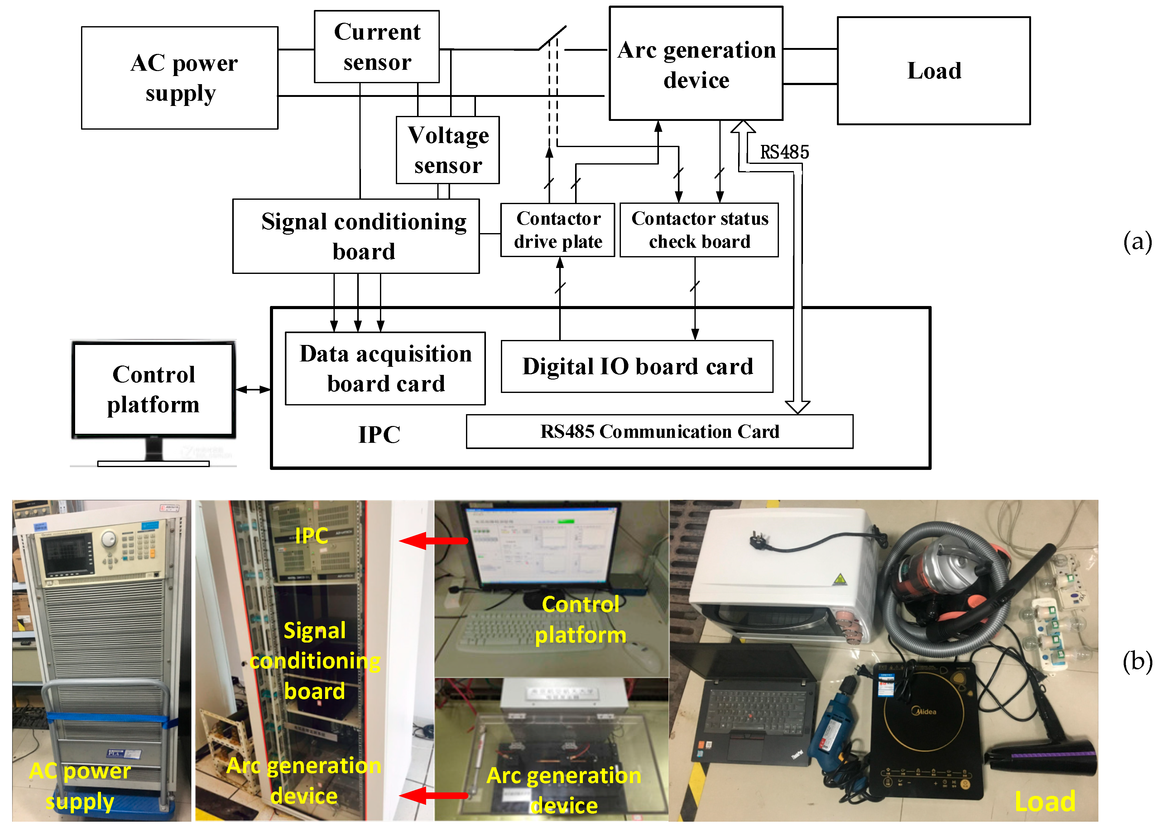
2. Experimental Platform and Data Acquisition
2.1. Experimental Platform
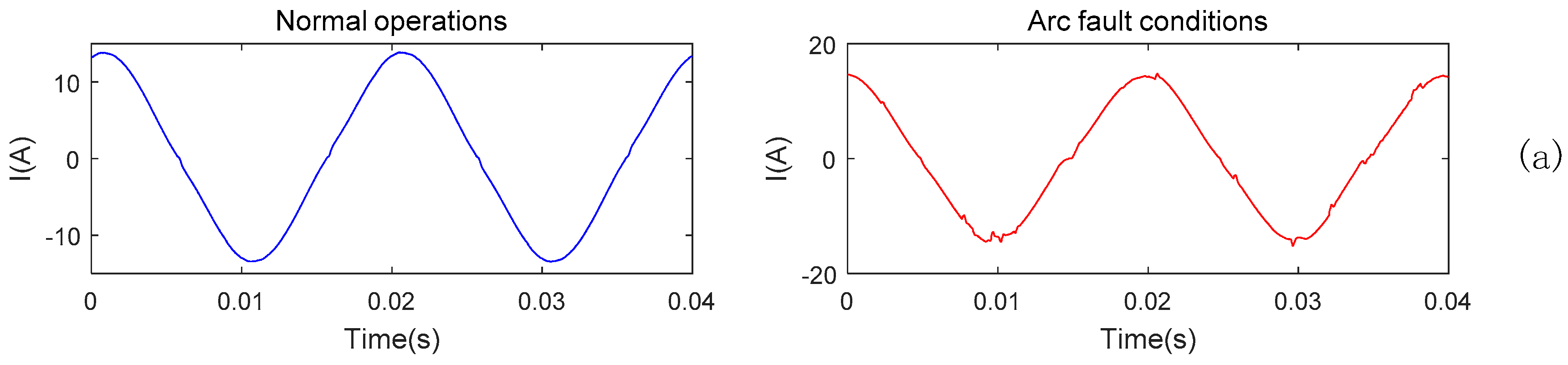
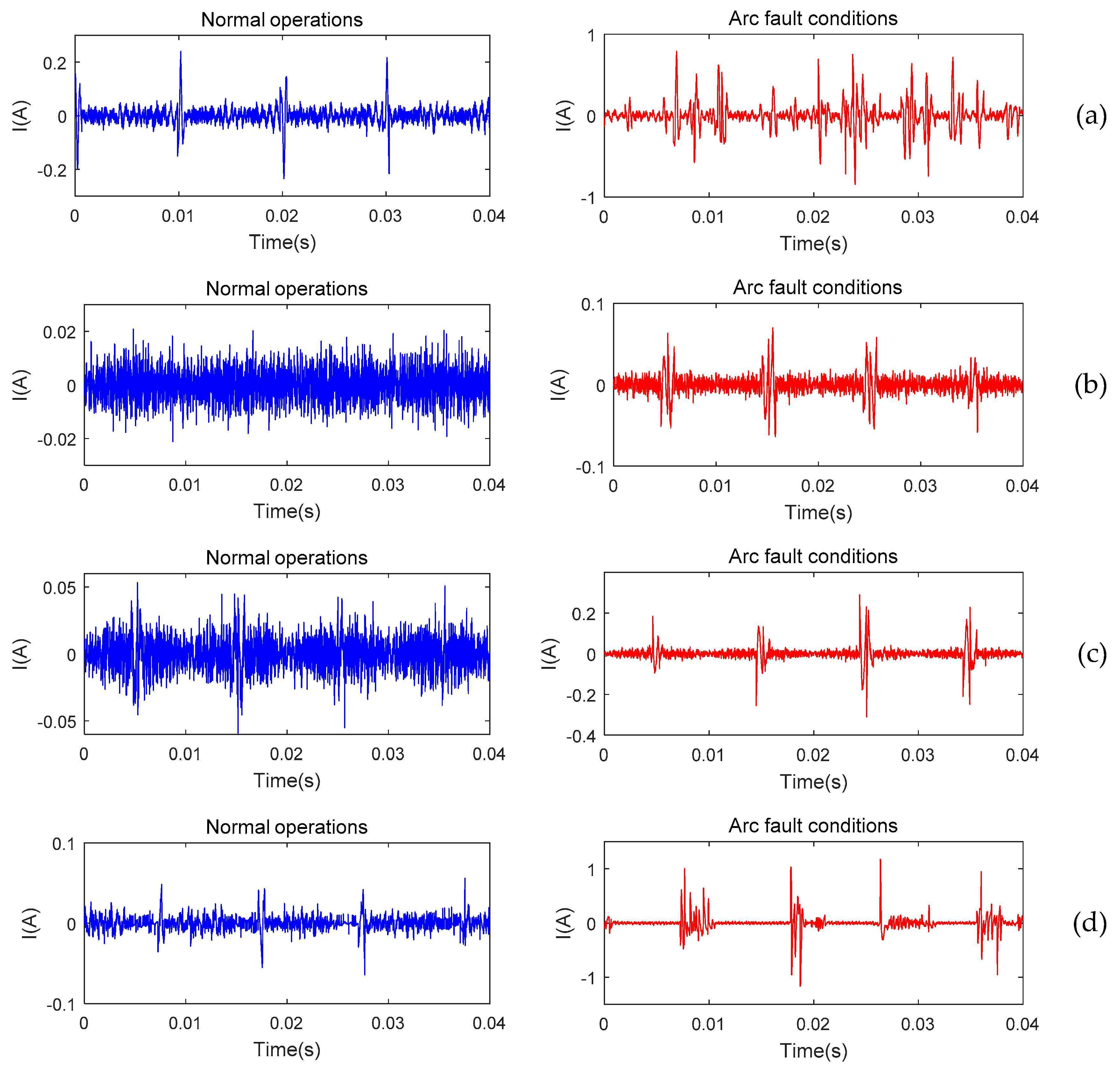
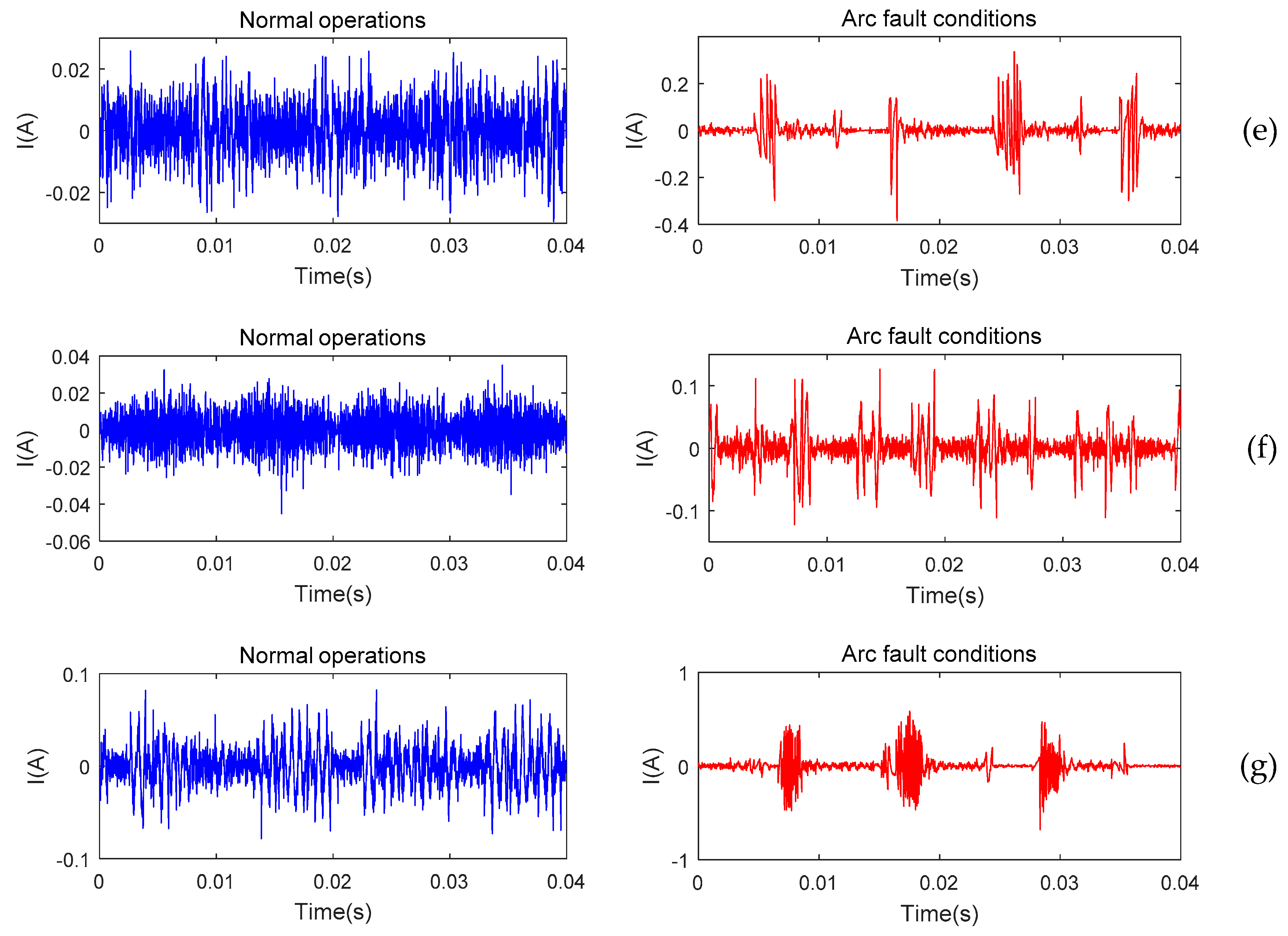
2.2. Experimental Data
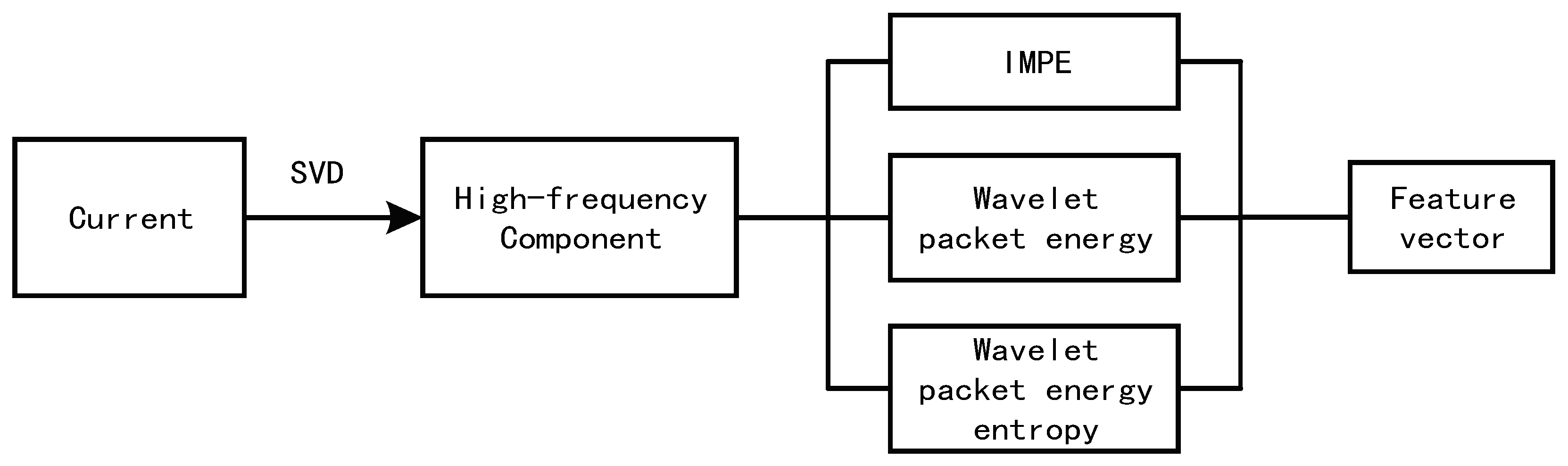
3. Feature Extraction
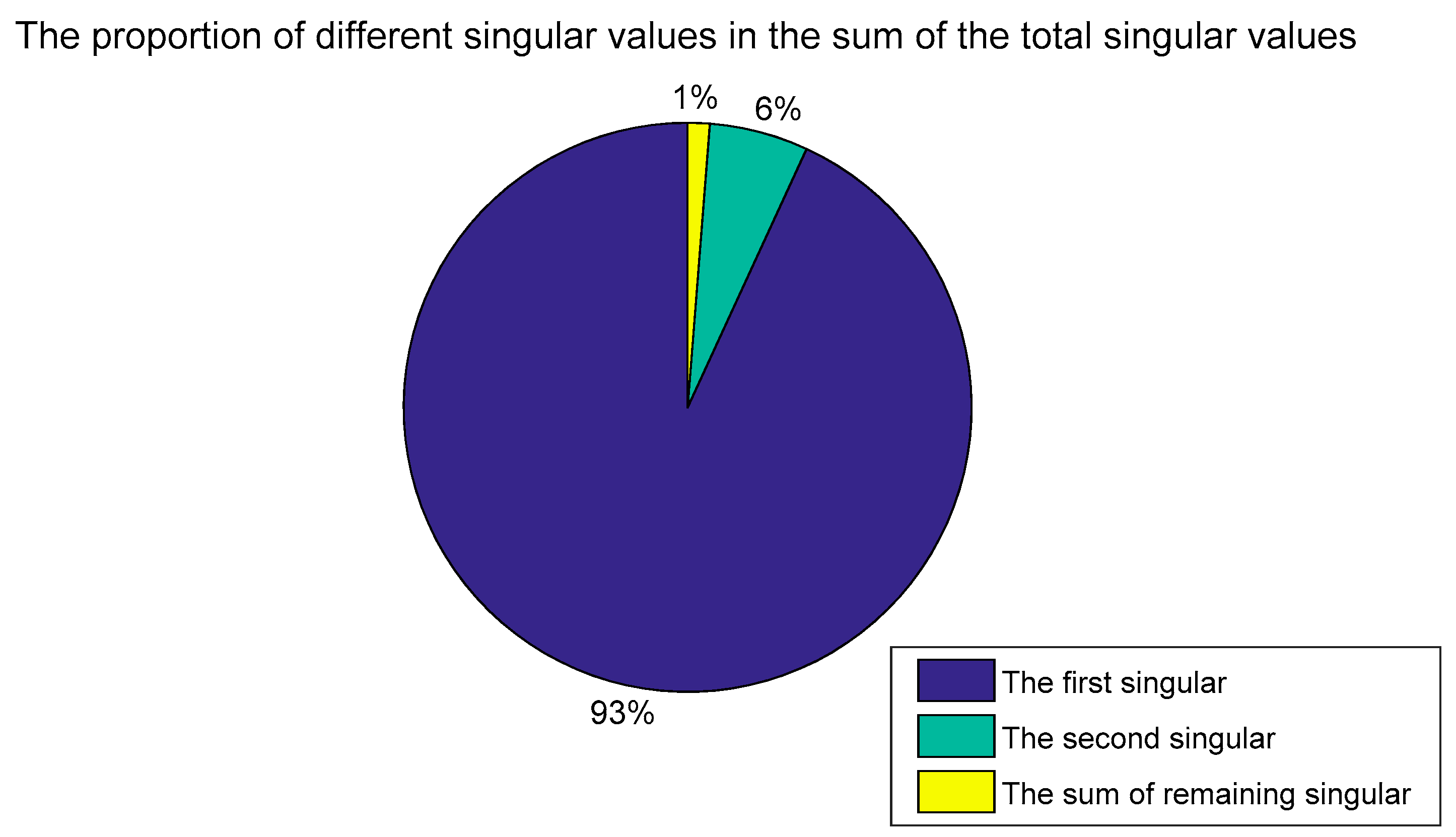
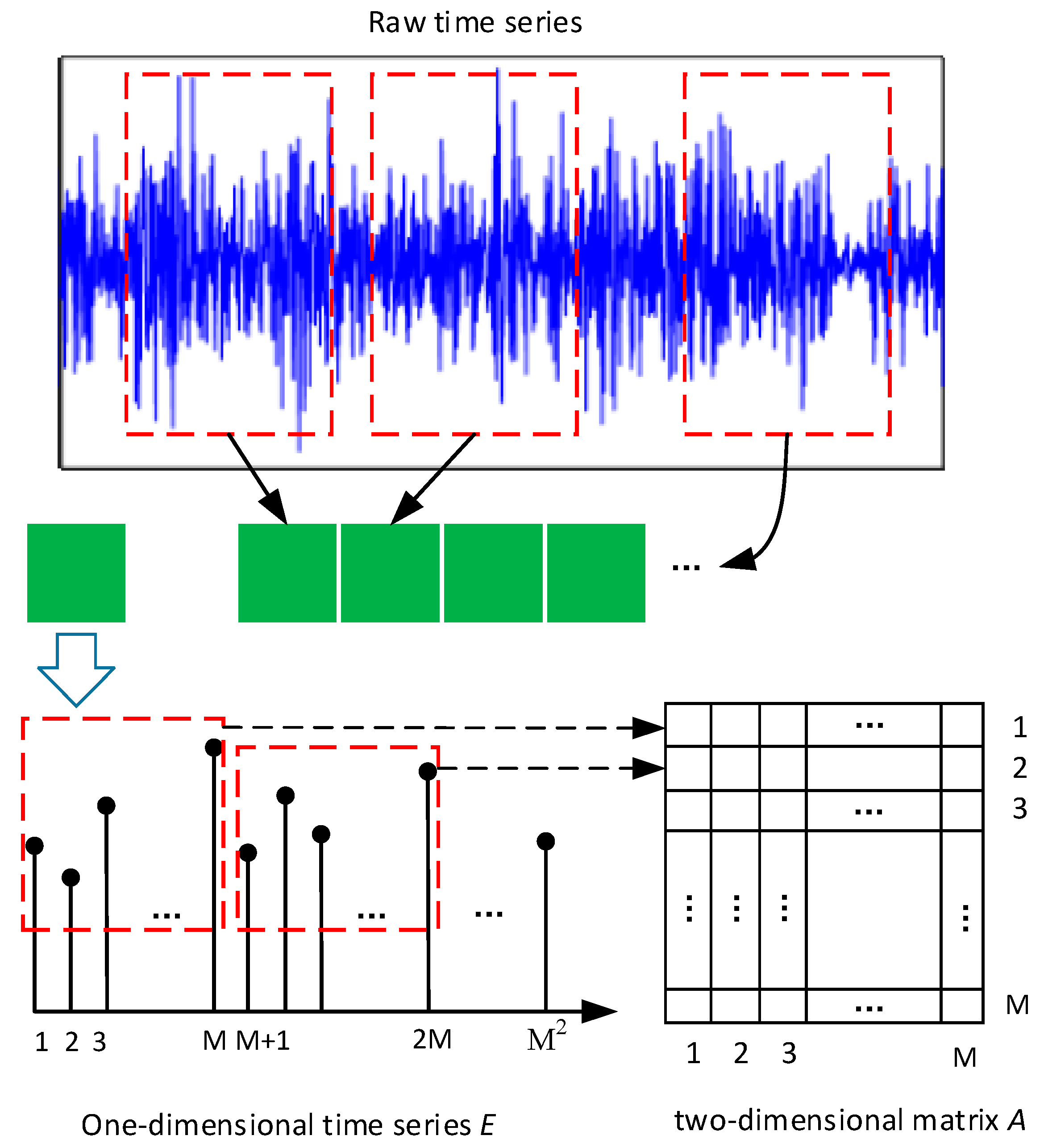
3.1. SVD
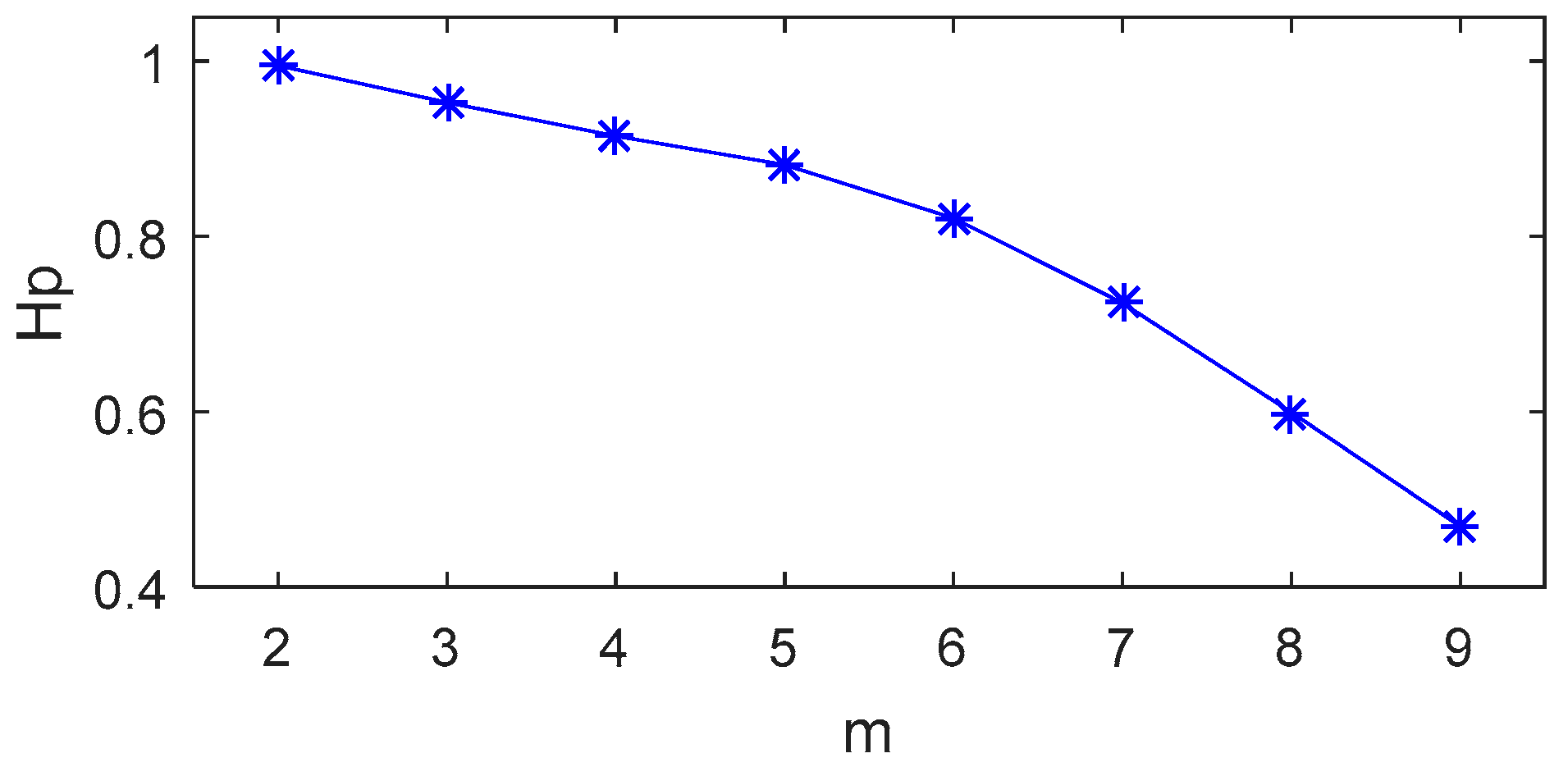
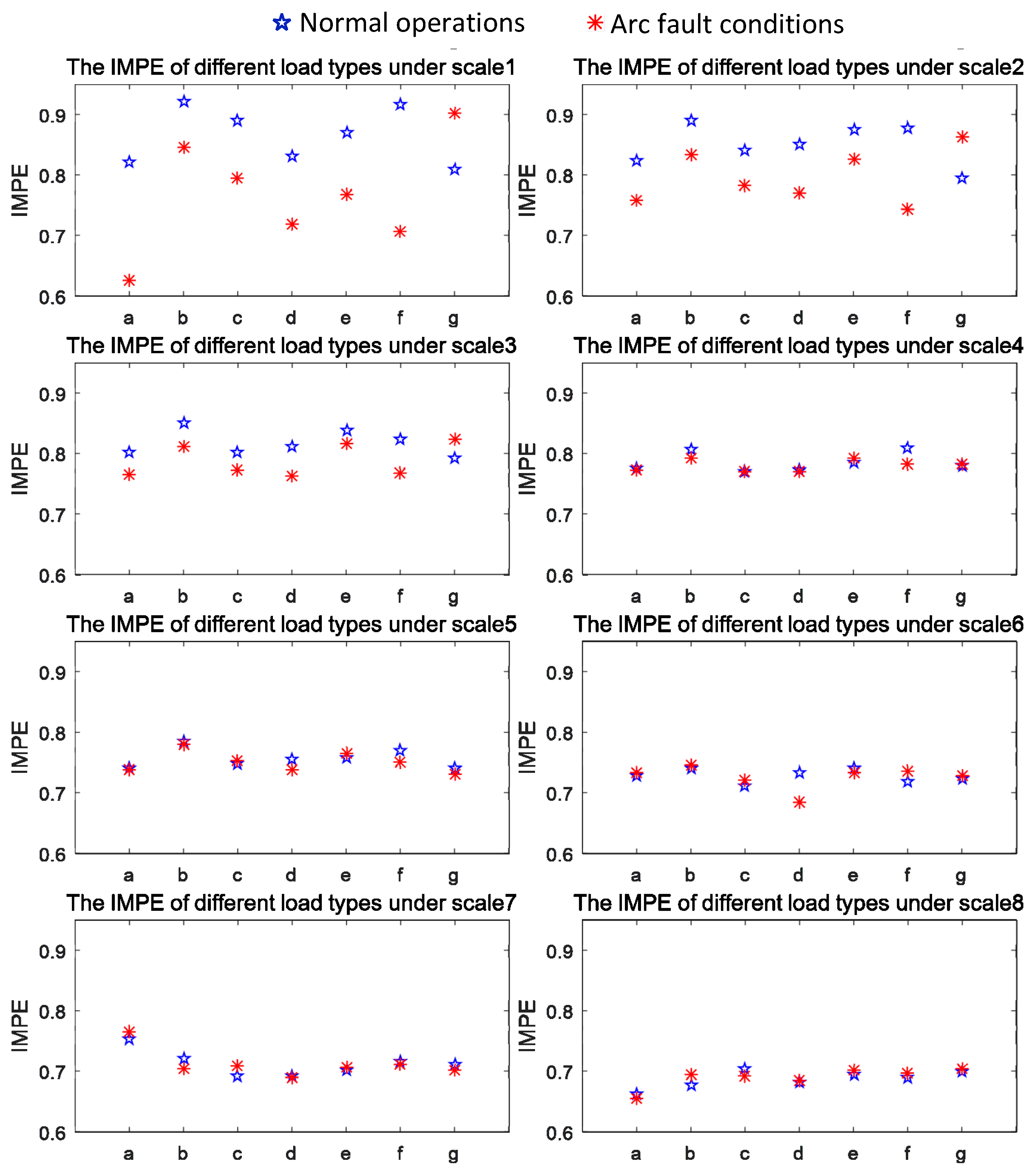
3.2. IMPE
3.2.1. PE
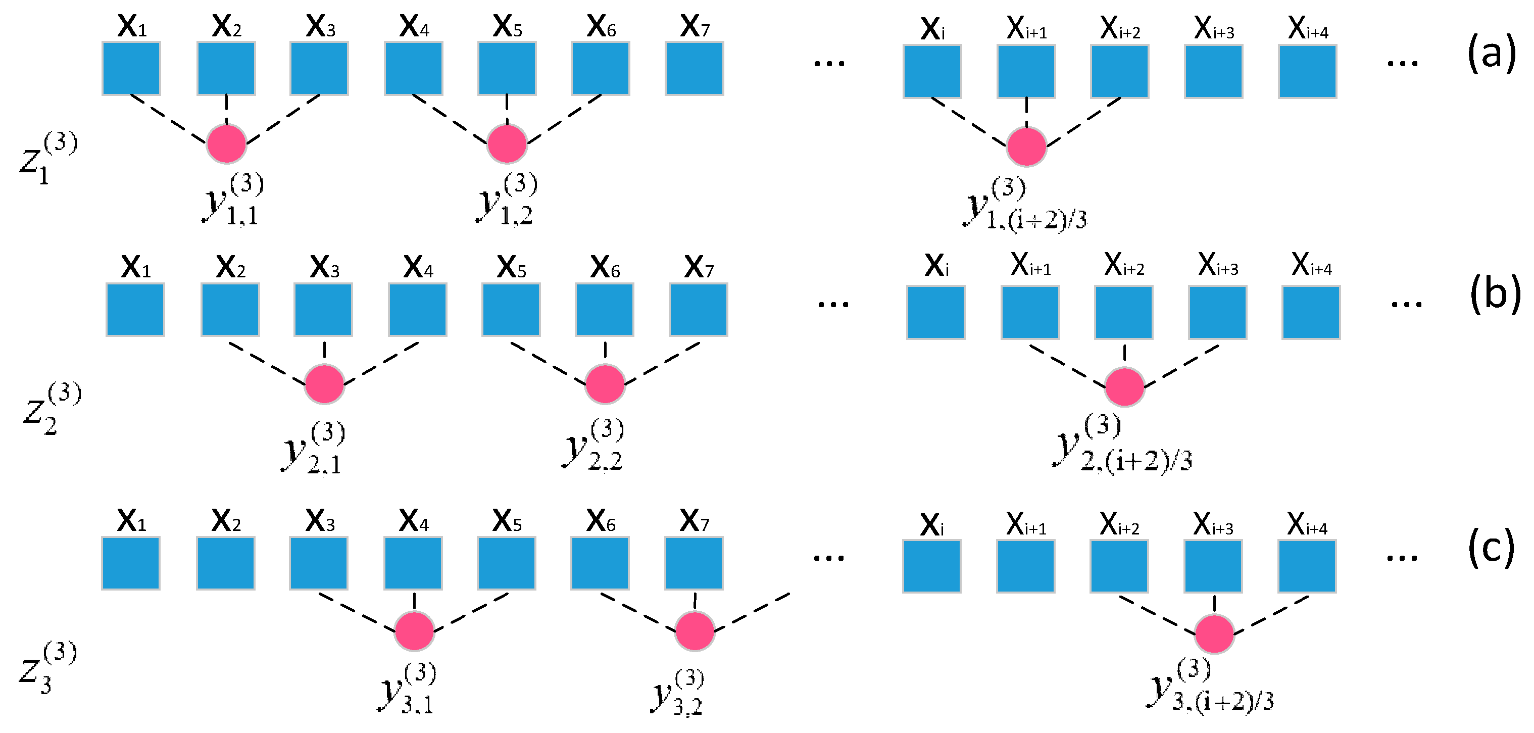
3.2.2. IMPE
3.2.3. The Feature Extraction of IMPE
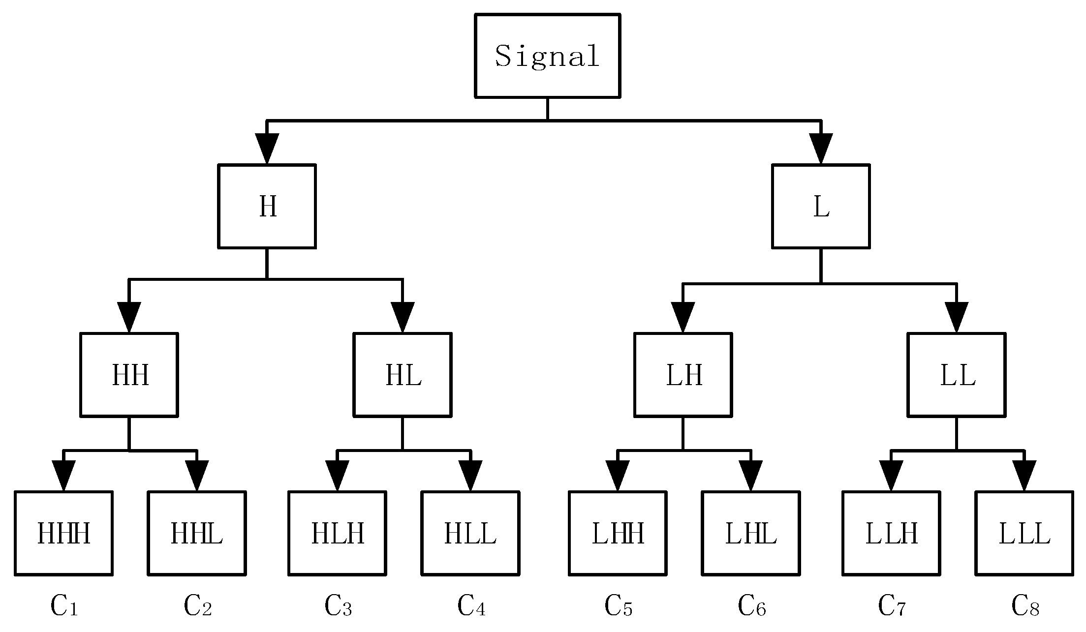
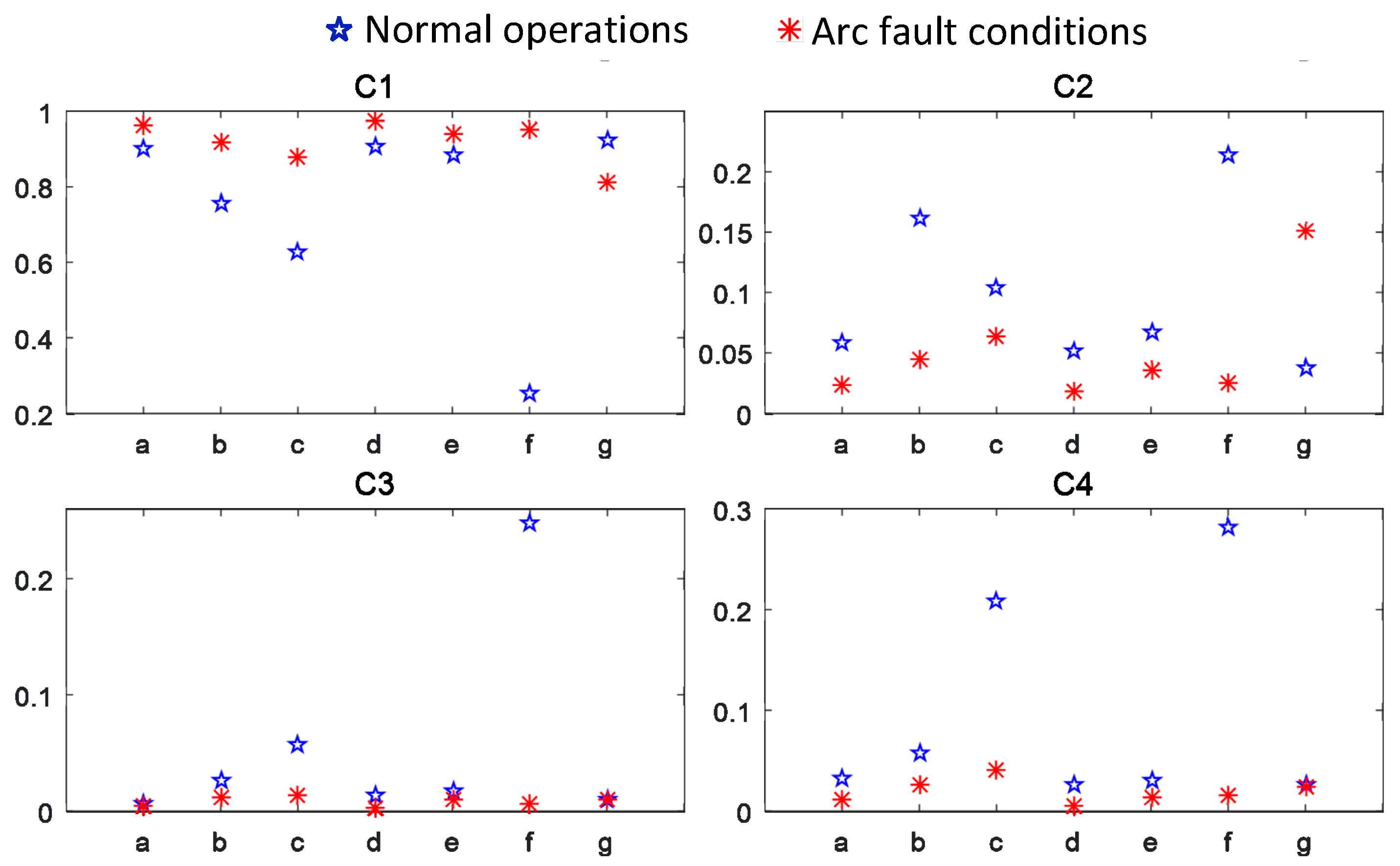
3.3. WPT
4. The Detection of Serial Arc Fault
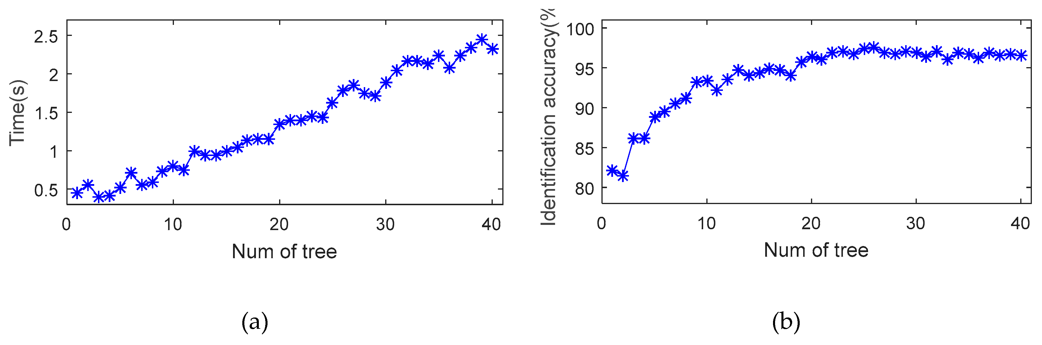
4.1. RF
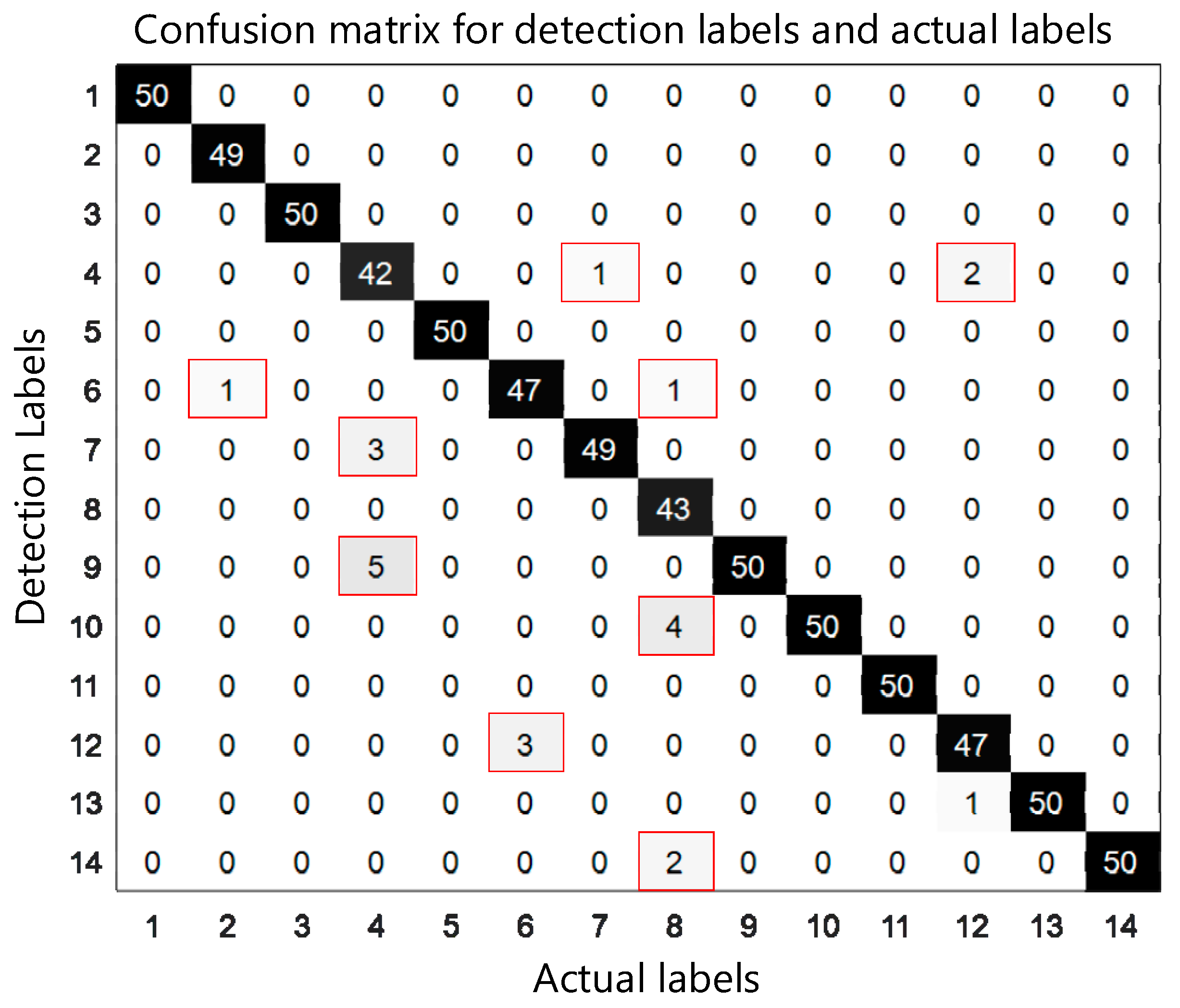
4.2. Analysis of detection results
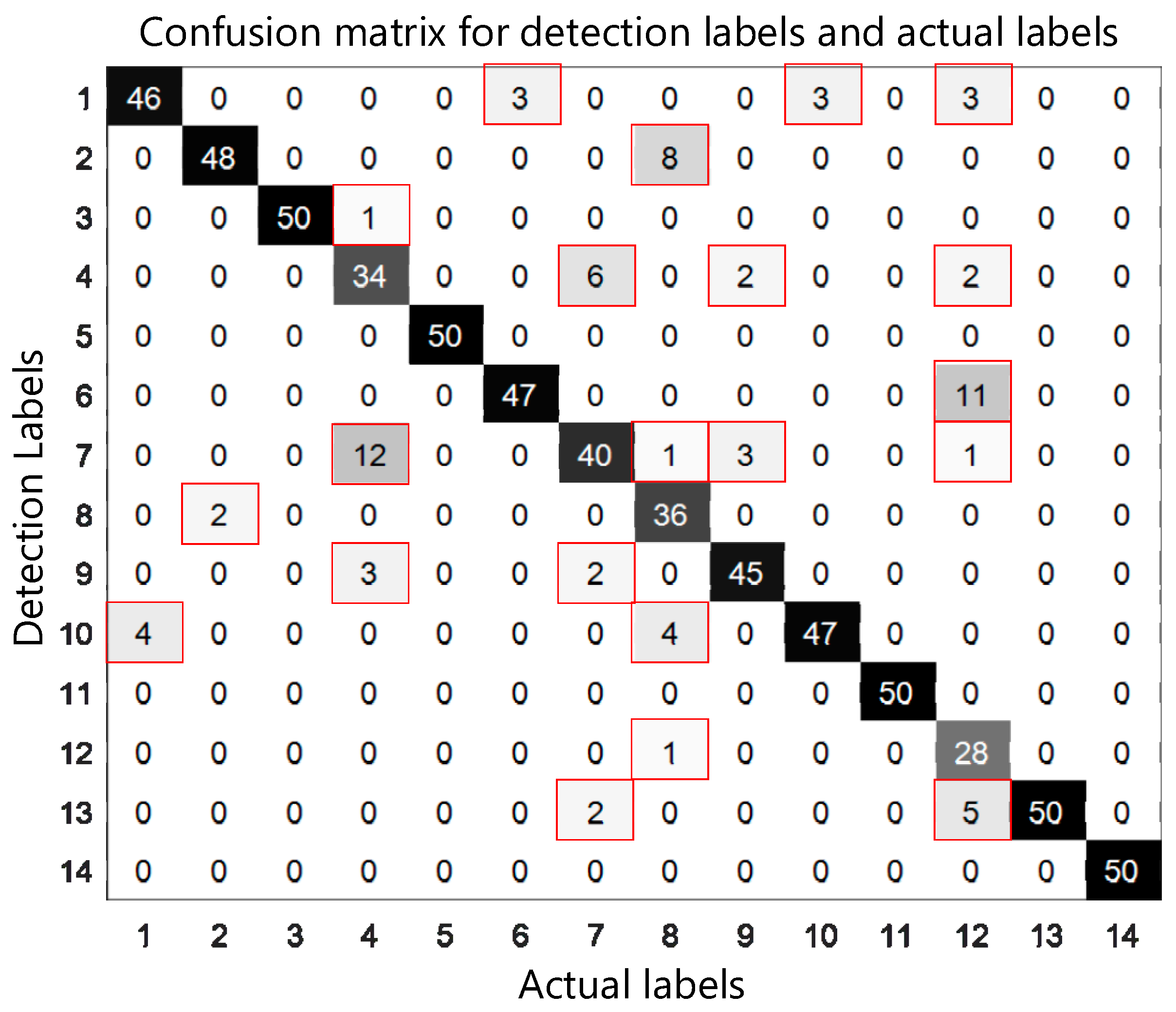
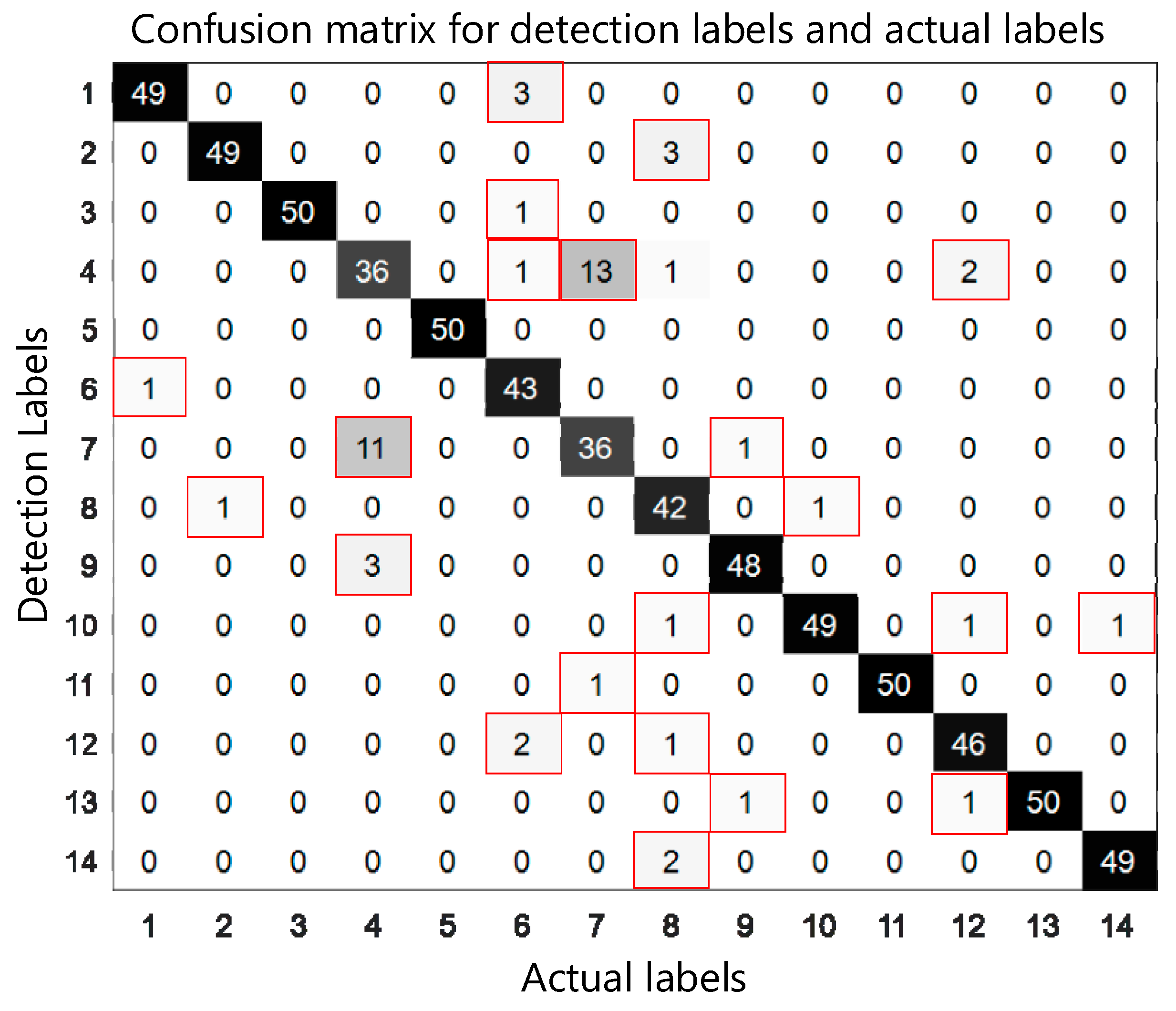
4.3. Comparison with Prior Methods
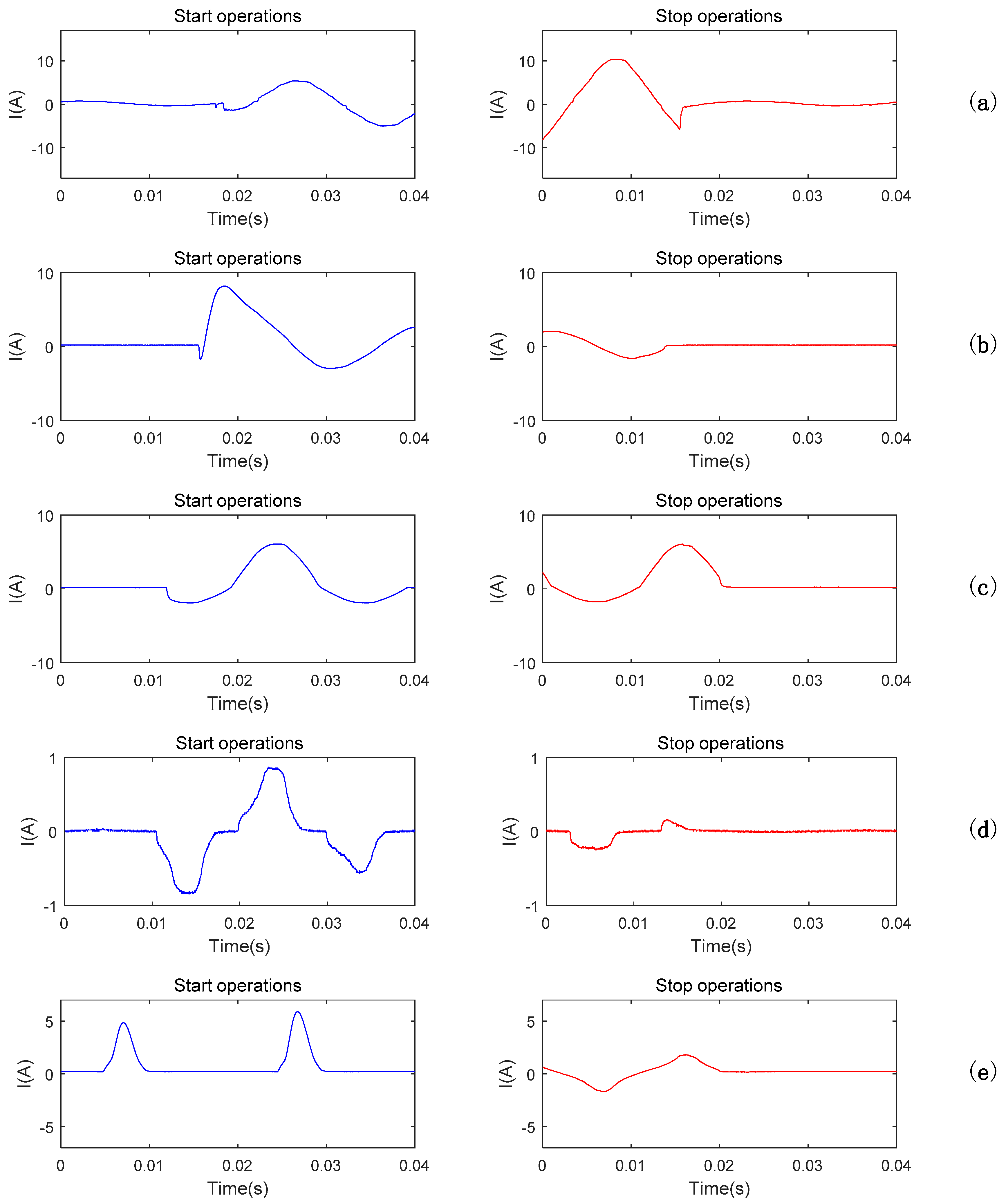
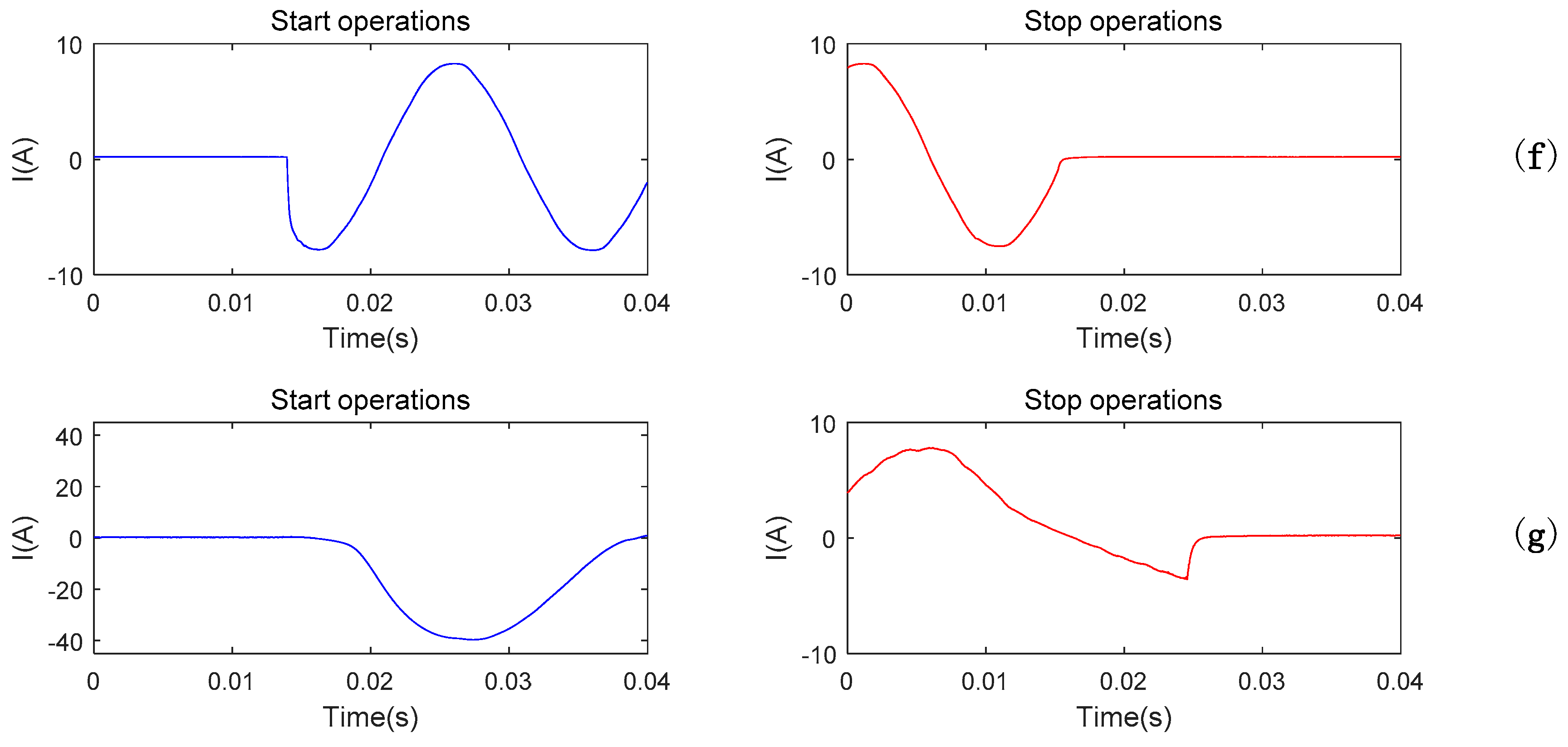
4.4. The Experiments of Transient Events
5. Conclusions
Author Contributions
Funding
Conflicts of Interest
References
- United States Fire Administration National Fire Data Center. Residential building fires (2013–2015). Top. Fire Rep. Ser. 2017, 16, 1–17. [Google Scholar]
- Fire Department of Ministry of Public Security. China Fire Services (2016); Yunnan People’s Publishing House: Kunming, China, 2016; pp. 396–407.
- United States Fire Administration National Fire Data Center. Residential building fires (2009–2011). Top. Fire Rep. Ser. 2014, 14, 1–11. [Google Scholar]
- Lee, R.H. The Other Electrical Hazard: Electric Arc Blast Burns. IEEE Trans. Ind. Appl. 1982, 246–251. [Google Scholar] [CrossRef]
- Gregory, G.D.; Scott, G.W. The arc-fault circuit interrupter: An emerging product. IEEE Trans. Ind. Appl. 1998, 34, 928–933. [Google Scholar] [CrossRef]
- Restrepo, C.E. Arc fault detection and discrimination methods. In Proceedings of the Electrical Contacts-2007 53rd IEEE Holm Conference on Electrical Contacts, Pittsburgh, PA, USA, 16–19 September 2007; IEEE: New Orleans, LA, USA, 2007; pp. 115–122. [Google Scholar]
- Lippert, K.J.; Domitrovich, T.A. AFCIs—From a standards perspective. IEEE Trans. Ind. Appl. 2014, 50, 1478–1482. [Google Scholar] [CrossRef]
- Gregory, G.; Wong, K.; Dvorak, R. More about arc-fault circuit interrupters. IEEE Trans. Ind. Appl. 2004, 40, 1006–1011. [Google Scholar] [CrossRef]
- Jiang, B.-F.; Wang, L. Research on Arc Model in AC Low-voltage Electrical Wire Fault. Proc. Chin. Soc. Univ. Electr. Pow. Syst. Autom. 2009, 4, 50. [Google Scholar]
- Wang, QL.; Wang, B.W.; Guan, L.H.; Zhao, Z.Z. Model and experiment of low-voltage AC series fault arc. Chin. Soc. Univ. Electr. Pow. Syst. Autom. 2018, 30, 26–35. [Google Scholar]
- Lan, H.-L.; Zhang, R.-C. Study on the feature extraction of fault arc sound signal based on wavelet analysis. Proc. Chin. Soc. Univ. Electr. Pow. Syst. Autom. 2008, 4, 57–62. [Google Scholar]
- Kim, C.J. Electromagnetic Radiation Behavior of Low-Voltage Arcing Fault. IEEE Trans. Deliv. 2009, 24, 416–423. [Google Scholar] [CrossRef]
- Zhang, R.C.; Yang, J.; Du, J.H. Study on In-Process Detection and Diagnosis of Faults Arc Based on Early Sounds Signature and Intermittent Chaos. Key Eng. Mater. 2008, 381, 611–614. [Google Scholar] [CrossRef]
- Meyar-Naimi, H.; Hasanzadeh, S.; Sanaye-Pasand, M. Discrimination of arcing faults on overhead transmission lines for single-pole auto-reclosure. Int. Trans. Electr. Energy 2013, 23, 1523–1535. [Google Scholar] [CrossRef]
- Zhang, L.P.; Miao, X.R.; Shi, D.Y. Control, Research on low voltage arc fault recognition method based on EMD and ELM. Electric. Mach. Control 2016, 20, 54–60. [Google Scholar]
- Jia, K.; Ren, Z.; Bi, T.; Yang, Q. Ground fault location using the low voltage side recorded data in distribution systems. IEEE Trans. Ind. Appl. 2015, 51, 1. [Google Scholar] [CrossRef]
- Ukil, A. Detection of direction change in prefault current in current-only directional overcurrent protection. In Proceedings of the Conference of the IEEE Industrial Electronics Society, Florence, Italy, 23–26 October 2016; pp. 3829–3833. [Google Scholar]
- Fan, R.; Liu, Y.; Huang, R.; Diao, R.; Wang, S. Precise Fault Location on Transmission Lines Using Ensemble Kalman Filter. IEEE Trans. Deliv. 2018, 33, 3252–3255. [Google Scholar] [CrossRef]
- Lu, Q.; Wu, H.; Wang, S.; Kong, D. Research on Arc-Fault Detection Based on Difference-Root Mean Square Method; Low Voltage Apparatus: Shanghai, China, 2013; pp. 6–10. [Google Scholar]
- Cai, X. Research on Arc Fault Detection and Protection Technique in the AC Supply System. Master’s Thesis, Nanjing University of Aeronautics and Astronautics, Nanjing, China, 2013. [Google Scholar]
- Zhang, S.; Zhang, F.; Liu, P.; Han, Z. Series Arc Fault Identification Method Based on Energy Produced by Wavelet Transformation and Neural Network. Trans. China Electrotech. Soc. 2014, 29, 290–295. [Google Scholar]
- Kawady, T.A.; Elkalashy, N.I.; Ibrahim, A.E.; Taalab, A.-M.I. Arcing fault identification using combined Gabor Transform-neural network for transmission lines. Int. J. Electr. Syst. 2014, 61, 248–258. [Google Scholar] [CrossRef]
- Liu, Y.-W.; Wu, C.-J.; Wang, Y.-C. Detection of serial arc fault on low-voltage indoor power lines by using radial basis function neural network. Int. J. Electr. Syst. 2016, 83, 149–157. [Google Scholar] [CrossRef]
- Lu, Q.W.; Wang, T.; Li, Z.R.; Wang, C. Detection Method of Series Arcing Fault Based on Wavelet Transform and Singular Value Decomposition. Trans. China Electrotech. Soc. 2017, 17, 212–221. [Google Scholar]
- Guo, F.Y.; Deng, Y.; Wang, Z.Y.; You, J.L.; Gao, H.X. Series Arc Fault Characteristics Based on Gray Level-Gradient Co-Occurrence Matrix. Trans. China Electrotech. Soc. 2018, 33, 71–81. [Google Scholar]
- Wang, Y.; Zhang, F.; Zhang, S. A New Methodology for Identifying Arc Fault by Sparse Representation and Neural Network. IEEE Trans. Instrum. Meas. 2018, 67, 2526–2537. [Google Scholar] [CrossRef]
- Ma, S.H.; Bao, J.Q.; Cai, Z.Y.; Meng, C.Y. A novel arc fault identification method based on information dimension and current zero. Proc. CSEE 2016, 36, 2572. (In Chinese) [Google Scholar]
- Yang, K.; Zhang, R.C.; Yang, J.H.; Du, J.H.; Chen, S.H.; Tu, R. Series arc fault diagnostic method based on fractal dimension and support vector machine. Trans. China Electrotech. Soc. 2016, 31, 70–77. [Google Scholar]
- Cheng, Q.; Tezcan, J.; Cheng, J. Confidence and prediction intervals for semiparametric mixed-effect least squares support vector machine. Recognit. Lett. 2014, 40, 88–95. [Google Scholar] [CrossRef]
- Gu, H.; Zhang, F.; Wang, Z.; Ning, Q.; Zhang, S. In Identification method for low-voltage arc fault based on the loose combination of wavelet transformation and neural network. In Proceedings of the 2012 Power Engineering and Automation Conference, Wuhan, China, 14–16 September 2012; pp. 1–4. [Google Scholar]
- Zhang, S.; Zhang, F.; Liu, P.; Han, Z. Identification of Low Voltage AC Series Arc Faults by using Kalman Filtering Algorithm. Elektronika ir Elektrotechnika 2014, 20, 51–57. [Google Scholar] [CrossRef]
- Surrel, Y. Design of algorithms for phase measurements by the use of phase stepping. Appl. Opt. 1996, 35, 51. [Google Scholar] [CrossRef]
- Kuai, M.; Cheng, G.; Pang, Y.; Li, Y. Research of Planetary Gear Fault Diagnosis Based on Permutation Entropy of CEEMDAN and ANFIS. Sensors 2018, 18, 782. [Google Scholar] [CrossRef]
- Zheng, J.; Pan, H.; Yang, S.; Cheng, J. Generalized composite multiscale permutation entropy and Laplacian score based rolling bearing fault diagnosis. Mech. Syst. Process. 2018, 99, 229–243. [Google Scholar] [CrossRef]
- Kreuzer, M.; Kochs, E.F.; Schneider, G.; Jordan, D. Non-stationarity of EEG during wakefulness and anaesthesia: Advantages of EEG permutation entropy monitoring. J. Clin. Monit. Comput. 2014, 28, 573–580. [Google Scholar] [CrossRef]
- Ravelo-García, A.G.; Navarro-Mesa, J.L.; Casanova-Blancas, U.; Martin-Gonzalez, S.; Quintana-Morales, P.; Guerra-Moreno, I.; Canino-Rodríguez, J.M.; Hernández-Pérez, E. Application of the Permutation Entropy over the Heart Rate Variability for the Improvement of Electrocardiogram-based Sleep Breathing Pause Detection. Entropy 2015, 17, 914–927. [Google Scholar] [CrossRef]
- Costa, M.; Goldberger, A.L.; Peng, C.K. Multiscale Entropy Analysis of Complex Physiologic Time Series. Phys. Rev. Lett. 2007, 89, 705–708. [Google Scholar] [CrossRef]
- Azami, H.; Escudero, J. Improved multiscale permutation entropy for biomedical signal analysis: Interpretation and application to electroencephalogram recordings. Biomed. Process. Control 2016, 23, 28–41. [Google Scholar] [CrossRef]
- Shuting, W.; Xiong, Z. Teager Energy-entropy Ratio of Wavelet Packet Transform and Its Application in Bearing Fault Diagnosis. Entropy 2018, 20, 388. [Google Scholar]
- Lin, S.; Liu, Z.; Hu, K. Traction Inverter Open Switch Fault Diagnosis Based on Choi–Williams Distribution Spectral Kurtosis and Wavelet-Packet Energy Shannon Entropy. Entropy 2017, 19, 504. [Google Scholar] [CrossRef]
- Cutler, A.; Cutler, D.R.; Stevens, J.R. Random Forests. Mach. Learn. 2004, 45, 157–176. [Google Scholar]
- Wang, Z.; Zhang, Q.; Xiong, J.; Xiao, M.; Sun, G.; He, J. Fault Diagnosis of a Rolling Bearing Using Wavelet Packet Denoising and Random Forests. IEEE Sens. J. 2017, 17, 5581–5588. [Google Scholar] [CrossRef]
- Cai, J.-D.; Yan, R.-W. Fault diagnosis of power electronic circuit based on random forests algorithm. In Proceedings of the 2009 Fifth International Conference on Natural Computation, Tianjian, China, 14–16 August 2009; pp. 214–217. [Google Scholar]
- Ko, B.C.; Gim, J.W.; Nam, J.Y. Cell image classification based on ensemble features and random forest. Electron. Lett. 2011, 47, 638. [Google Scholar] [CrossRef]
- Özçift, A. Random forests ensemble classifier trained with data resampling strategy to improve cardiac arrhythmia diagnosis. Comput. Boil. Med. 2011, 41, 265–271. [Google Scholar] [CrossRef]
- Liu, R.; Tan, T. An SVD-based watermarking scheme for protecting rightful ownership. IEEE Trans. Multimed. 2002, 4, 121–128. [Google Scholar]
- Do, V.T.; Chong, U.P. Signal Model-Based Fault Detection and Diagnosis for Induction Motors Using Features of Vibration Signal in Two-Dimension Domain. Stroj. Vestn-J Mech. E. 2011, 57, 655–666. [Google Scholar] [CrossRef]
- Wen, L.; Li, X.; Gao, L.; Zhang, Y. A New Convolutional Neural Network-Based Data-Driven Fault Diagnosis Method. IEEE Trans. Ind. Electron. 2018, 65, 5990–5998. [Google Scholar] [CrossRef]
- Salas, J.; Kim, H.; Eykholt, R. Nonlinear dynamics, delay times, and embedding windows. Phys. D Phenom. 1999, 127, 48–60. [Google Scholar]
- Pompe, B.; Bandt, C. Permutation Entropy: A Natural Complexity Measure for Time Series. Phys. Rev. Lett. 2002, 88, 174102. [Google Scholar]
- Cao, Y.; Tung, W.-W.; Gao, J.B.; Protopopescu, V.A.; Hively, L.M. Detecting dynamical changes in time series using the permutation entropy. Phys. Rev. E 2004, 70, 046217. [Google Scholar] [CrossRef]
- Yan, R.; Liu, Y.; Gao, R.X. Permutation entropy: A nonlinear statistical measure for status characterization of rotary machines. Mech. Syst. Process. 2012, 29, 474–484. [Google Scholar] [CrossRef]
- Zhang, X.; Liang, Y.; Zhou, J.; Zang, Y. A novel bearing fault diagnosis model integrated permutation entropy, ensemble empirical mode decomposition and optimized SVM. Measurement 2015, 69, 164–179. [Google Scholar] [CrossRef]


| Load Type | Operating Condition | |
|---|---|---|
| Operating Voltage/V | Power/W | |
| Induction cooker | 220 | 2100 |
| Incandescent lamp | 220 | 200 |
| Hairdryer | 220 | 2000 |
| Notebook computer | 220 | 148.3 |
| Electric drill | 220 | 600 |
| Electric oven | 220 | 1200 |
| Vacuum cleaner | 220 | 1200 |
| Load Type | Operating Condition | Scale1 | Scale2 | Scale3 | Scale4 | Scale5 | Scale6 | Scale7 | Scale8 |
|---|---|---|---|---|---|---|---|---|---|
| Induction cooker | Normal | 0.8209 | 0.8248 | 0.8017 | 0.7749 | 0.7416 | 0.7293 | 0.7523 | 0.6635 |
| Arc | 0.6264 | 0.7586 | 0.7662 | 0.7715 | 0.7381 | 0.7345 | 0.7664 | 0.6553 | |
| Incandescent lamp | Normal | 0.9220 | 0.8891 | 0.8516 | 0.8072 | 0.7838 | 0.7417 | 0.7207 | 0.6772 |
| Arc | 0.8468 | 0.8343 | 0.8114 | 0.7928 | 0.7795 | 0.7458 | 0.7048 | 0.6934 | |
| Hairdryer | Normal | 0.8893 | 0.8417 | 0.8015 | 0.7697 | 0.7491 | 0.7124 | 0.6929 | 0.7049 |
| Arc | 0.7951 | 0.7831 | 0.7727 | 0.7712 | 0.7518 | 0.7219 | 0.7101 | 0.6912 | |
| Notebook computer | Normal | 0.8311 | 0.8514 | 0.8123 | 0.7732 | 0.7546 | 0.7342 | 0.6927 | 0.6816 |
| Arc | 0.7186 | 0.7710 | 0.7617 | 0.7689 | 0.7395 | 0.6855 | 0.6893 | 0.6838 | |
| Electric drill | Normal | 0.8715 | 0.8744 | 0.8376 | 0.7853 | 0.7589 | 0.7403 | 0.7012 | 0.6953 |
| Arc | 0.7681 | 0.8272 | 0.8168 | 0.7917 | 0.7646 | 0.7342 | 0.7075 | 0.7010 | |
| Electric oven | Normal | 0.9168 | 0.8786 | 0.8243 | 0.8091 | 0.7698 | 0.7175 | 0.7174 | 0.6905 |
| Arc | 0.7056 | 0.7439 | 0.7683 | 0.7820 | 0.7512 | 0.7355 | 0.7108 | 0.6972 | |
| Vacuum cleaner | Normal | 0.8104 | 0.7945 | 0.7916 | 0.7799 | 0.7396 | 0.7247 | 0.7114 | 0.6985 |
| Arc | 0.9020 | 0.8619 | 0.8239 | 0.7817 | 0.7314 | 0.7286 | 0.7008 | 0.7049 |
| Load Type | Operating Condition | C1 | C2 | C3 | C4 | Wavelet Energy-Entropy |
|---|---|---|---|---|---|---|
| Induction cooker | Normal | 0.9027 | 0.0586 | 0.0067 | 0.0320 | 0.5805 |
| Arc | 0.9612 | 0.0236 | 0.0039 | 0.0113 | 0.2866 | |
| Incandescent lamp | Normal | 0.7541 | 0.1622 | 0.0266 | 0.0570 | 1.1076 |
| Arc | 0.9172 | 0.0445 | 0.0117 | 0.0266 | 0.5286 | |
| Hairdryer | Normal | 0.6285 | 0.1042 | 0.0577 | 0.2096 | 1.4709 |
| Arc | 0.8822 | 0.0637 | 0.0133 | 0.0408 | 0.6837 | |
| Notebook computer | Normal | 0.9100 | 0.0512 | 0.0135 | 0.0252 | 0.5612 |
| Arc | 0.9725 | 0.0192 | 0.0024 | 0.0059 | 0.2132 | |
| Electric drill | Normal | 0.8855 | 0.0668 | 0.0180 | 0.0296 | 0.6709 |
| Arc | 0.9403 | 0.0357 | 0.0100 | 0.0140 | 0.4078 | |
| Electric oven | Normal | 0.2544 | 0.2140 | 0.2488 | 0.2828 | 1.9930 |
| Arc | 0.9520 | 0.0262 | 0.0063 | 0.0155 | 0.3445 | |
| Vacuum cleaner | Normal | 0.9265 | 0.0380 | 0.0103 | 0.0253 | 0.4832 |
| Arc | 0.8149 | 0.1504 | 0.0106 | 0.0241 | 0.8509 |
| Load Type | Operating Condition | Label | Number of Test Set | Number of Correctly Detected | Detection Accuracy/% |
|---|---|---|---|---|---|
| Induction cooker | Normal | 1 | 50 | 50 | 100 |
| Arc | 2 | 50 | 49 | 98 | |
| Incandescent lamp | Normal | 3 | 50 | 50 | 100 |
| Arc | 4 | 50 | 42 | 84 | |
| Hairdryer | Normal | 5 | 50 | 50 | 100 |
| Arc | 6 | 50 | 47 | 94 | |
| Notebook computer | Normal | 7 | 50 | 49 | 98 |
| Arc | 8 | 50 | 43 | 86 | |
| Electric drill | Normal | 9 | 50 | 50 | 100 |
| Arc | 10 | 50 | 50 | 100 | |
| Electric oven | Normal | 11 | 50 | 50 | 100 |
| Arc | 12 | 50 | 47 | 94 | |
| Vacuum cleaner | Normal | 13 | 50 | 50 | 100 |
| Arc | 14 | 50 | 50 | 100 |
| Classifier | The Number of Test Data | The Number of Correctly Detected | Detection Accuracy under Normal Operations (%) | Detection Accuracy under Serial arc Fault Conditions (%) | Detection Accuracy (%) |
|---|---|---|---|---|---|
| BPNN | 700 | 621 | 94.57 | 80 | 88.71 |
| LSSVM | 700 | 644 | 95.14 | 89.71 | 92.43 |
| RF | 700 | 677 | 99.71 | 93.71 | 96.71 |
| Load Type | Operating Condition | Number of Samples | Number of Correctly Detected | Detection Accuracy/% |
|---|---|---|---|---|
| Induction cooker | Start | 20 | 20 | 100 |
| Stop | 20 | 19 | 95 | |
| Incandescent lamp | Start | 20 | 20 | 100 |
| Stop | 20 | 20 | 100 | |
| Hairdryer | Start | 20 | 20 | 100 |
| Stop | 20 | 20 | 100 | |
| Notebook computer | Start | 20 | 20 | 100 |
| Stop | 20 | 20 | 100 | |
| Electric drill | Start | 20 | 20 | 100 |
| Stop | 20 | 20 | 100 | |
| Electric oven | Start | 20 | 20 | 100 |
| Stop | 20 | 20 | 100 | |
| Vacuum cleaner | Start | 20 | 20 | 100 |
| Stop | 20 | 20 | 100 |
© 2019 by the authors. Licensee MDPI, Basel, Switzerland. This article is an open access article distributed under the terms and conditions of the Creative Commons Attribution (CC BY) license (http://creativecommons.org/licenses/by/4.0/).
Share and Cite
Yin, Z.; Wang, L.; Zhang, Y.; Gao, Y. A Novel Arc Fault Detection Method Integrated Random Forest, Improved Multi-scale Permutation Entropy and Wavelet Packet Transform. Electronics 2019, 8, 396. https://doi.org/10.3390/electronics8040396
Yin Z, Wang L, Zhang Y, Gao Y. A Novel Arc Fault Detection Method Integrated Random Forest, Improved Multi-scale Permutation Entropy and Wavelet Packet Transform. Electronics. 2019; 8(4):396. https://doi.org/10.3390/electronics8040396
Chicago/Turabian StyleYin, Zhendong, Li Wang, Yaojia Zhang, and Yang Gao. 2019. "A Novel Arc Fault Detection Method Integrated Random Forest, Improved Multi-scale Permutation Entropy and Wavelet Packet Transform" Electronics 8, no. 4: 396. https://doi.org/10.3390/electronics8040396
APA StyleYin, Z., Wang, L., Zhang, Y., & Gao, Y. (2019). A Novel Arc Fault Detection Method Integrated Random Forest, Improved Multi-scale Permutation Entropy and Wavelet Packet Transform. Electronics, 8(4), 396. https://doi.org/10.3390/electronics8040396