1. Introduction
A fatal crash occurred in a Tesla Model S on 5 July 2016. This was the first known fatality in autopilot on an autonomous vehicle. Tesla noted that “the vehicle was on a divided highway with Autopilot engaged when a tractor trailer drove across the highway perpendicular to the Model S. Neither Autopilot nor the driver noticed the white side of the tractor trailer against a brightly lit sky, so the brake was not applied.” [
1]. There are three sensor systems in Tesla Autopilot. The first one is the vision system named MobileEyeQ3 in the middle of the windshield. The second is the millimeter-wave radar below the front bumper. The last one is twelve ultrasonic sensors around the vehicle. All sensors unfortunately missed the back part during the unusual situation in which the fatality occurred. The measuring distance of the ultrasonic radar was too short (2 m). It could not detect obstructions at high speeds. The installed position of the millimeter-wave radar system was too low, and its vertical angle was less than five degrees, thus this sensor missed the object. Optical detection ideally emulates how human observes the world and therefore should be the most efficient method. However, it is difficult for the camera to extract features of white objects from a large white background. It cannot get enough feature information to input the MobiEyeQ3. This results in the MobiEyeQ3 missing the object. Essentially, the problem is caused by less redundancy of the image algorithm. In addition, if a large part of the vehicle is similar to blue sky, buildings, or trees, the computer vision system of the self-driving car could miss detecting the part.
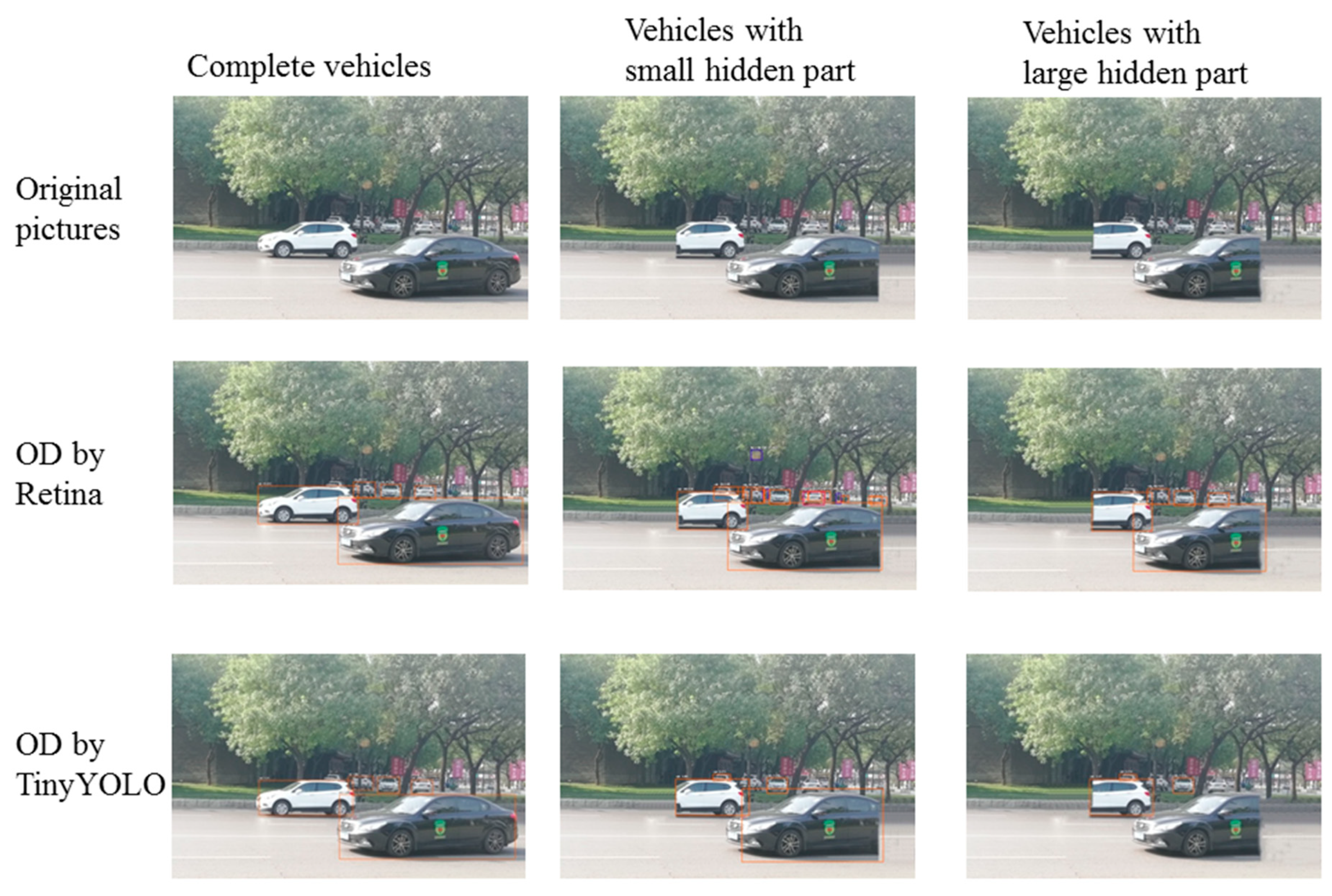
The left picture in the first row of
Figure 1 was taken from a real scene. According to the Tesla accident report [
1], the extreme virtual environment was settled. In this virtual environment, two virtual cars are shown in the middle and right of the first row. Let us postulate that the drivers paint the back of the black car and the front of the white SUV in a color and style that match completely with the background. Thus, the painted parts blend into the background and cannot be seen but exist nonetheless. This type of vehicle is rare in the real world and looks ridiculous. However, they cannot be excluded.
In this particular case, almost all of the object detection algorithms would fail. The second and third row respectively show the results processed by the latest object detection algorithms, Retina [
2] and TinyYOLO [
3]. In
Figure 1, the abbreviation “OD” stands for “object detection”. Both algorithms failed to detect the entire vehicle in columns 2 and 3.
Figure 1 demonstrates that the state of the art object detection algorithms cannot detect the hidden part. If these special vehicles are encountered in the real word, an aforementioned accident will still occur.
The research tries to solve the above problem by deep learning networks. Recently, with the successful application of machine learning, deep learning is becoming more effective in various fields. The researchers use deep neural networks for image classification [
4,
5,
6,
7], semantic segmentation [
8,
9], object detection [
2,
3,
10], image generation [
11], etc. We propose a novel method to detect the hidden part of a vehicle, thus helping to avoid traffic accidents. In other words, we learn to “see” the hidden part.
Our proposed algorithm tried to correctly handle the situation in the extreme condition shown in
Figure 1. Firstly, the deep learning network model needed to be trained on an enormous number of images to achieve satisfactory performance. We collected vehicle pictures by the camera in the busiest streets of the ancient city, Xi’an, China. In addition to our database, we prepared the other databases described in detail in
Section 4.1.
After the databases were prepared, an improved Retina object detection model was trained for detecting the vehicles. In the unmanned vehicle scene, quickly identifying objects is necessary. Recently, real-time object detection methods such as Retina network [
2] and YOLO network [
3,
10] have been proposed. To increase the performance of detecting speed and keep the safety level, a detection model with high threshold value was created. This model is used in the first stage of object detection. The proposed algorithm does not know whether or not the front vehicles have the hidden part beforehand. There is no signal “telling” the algorithm whether or not the vehicle has hidden parts. A reasonable assumption is made that all vehicles may have hidden parts. For reducing the computational work, the main vehicles in the middle of the road are detected by this model. The vehicles that occur further in the distance are not likely to cause accidents and can be ignored. An image inpainting model for inpainting the vehicles was created. Assuming the detected vehicles have hidden parts that cannot be seen by a general computer vision system, inpainting the right and left area is applied separately. When the inpainting algorithm is applied to a complete vehicle without any hidden part, inpainting does not add anything. Otherwise, the area of the inpainted vehicle increases. Then, a second stage of object detection is immediately applied to the inpainted vehicle with the same improved Retina model. The difference between the first and second stage of detected regions is defined as an alarm box. This time, the hidden part can be “seen”. The alarm box is the existing region that the normal visual system cannot detect. Vehicles should avoid the alarm box region.
The whole procedure is called the DIDA approach (object detection, inpainting, object re-detection, setting alarm box). We show experimentally that the proposed DIDA can “see” the part that cannot be detected by typical optical systems in
Section 3.
Our contributions in this paper are summarized as follows: (1) we proposed the DIDA approach to solve the problem of detecting the incomplete object in the autopilot scene; (2) we proposed the DIDA approach to “see” the hidden part of the vehicle using the serial joint processing of object detection and image inpainting, solving the aforementioned problem with only optical sensor signals for the first time and offering a new method for insuring further security in the autopilot system; (3) we collected the vehicle database in Xi’an, China, which can be used in subsequent research as well.
The rest of the paper is organized as follows. Related work on object detection and image inpainting is proposed in
Section 2. Methods such as the flow chart about seeing hidden parts of the vehicle, the framework of the object detection model, and Generative Adversarial Nets (GANs) [
12] are shown in
Section 3. Detailed experimental results are shown in
Section 4. Several problems that need to be further studied are addressed in
Section 5. The conclusions are described in
Section 6.
2. Related Work
This section provides an overview of research on object detection and image inpainting.
First of all, the research of object detection based on deep learning is reviewed. Each object detection model has essentially two phases—an object localization phase to search for candidate objects and a classification phase where the candidates are classified based on distinctive features. In the Region-based-Convolutional-Neural-Network-features (R-CNN) model [
13], the selective search method (SS) [
14] is used as an alternative to exhaustively searching for object localization. In particular, about 2000 small region proposals are generated and then merged in a bottom-up manner to obtain more accurate candidate regions. Different color-space features, saliency cues, and similarity metrics are used to guide the merging procedure. Each proposed region is then resized to match the input of the CNN model. The output of this model is a 4096-dimensional feature vector. To get the class probabilities, this generated feature vector needs to be classified by multiple Support Vector Machine (SVM) [
15]. The R-CNN model has achieved a 62.4% mean Average Precision (mAP) score on the PASCAL VOC 2012 [
16] benchmark and a 31.4% mAP score on the 2013 ImageNet [
17] benchmark in the large scale visual recognition challenge (ILSVRC).
The major limitation of this method is that it requires a long time to analyze the proposed regions. For addressing the weakness of the time-consuming analysis process, R. Girshick introduced the Fast Region-based Convolutional Network (Fast R-CNN) [
18]. The Fast R-CNN method produces output vectors that are further classified by a normalized exponential function (softmax) [
19] classifier. Experimental results proved that Fast R-CNNs were capable of achieving a mAP score of 70.0% and 68.4% on the 2007 and 2012 PASCAL VOC benchmarks, respectively.
To address the limitation of high computational overhead in the prior region based methods using selective search, the Region Proposal Network (RPN) [
20] were proposed, which produce region proposals directly by determine bounding boxes and detecting objects. This method led to the development of the Faster Region-based Convolutional Network (Faster R-CNN) [
20] as a combination of the RPN and the Fast R-CNN models. Experimental results of Faster R-CNN proved an improvement by reporting the mAP scores of 78.8% and 75.9% on the 2007 and 2012 PASCAL VOC benchmarks, respectively. The results of Faster R-CNN are computed 34 times faster than the original Fast R-CNN.
The two models mentioned above involve detection of region proposals and finding an object in the image. However, the Region-based Fully Convolutional Network (R-FCN) [
21] uses only convolutional back-propagation layers for learning and inference. The R-FCN reached an 83.6% mAP score on the 2007 PASCAL VOC benchmark. For the 2015 COCO [
22] challenge, this method reached a 53.2% score for an Intersection over Union (IoU) = 0.5 and a 31.5% score for the official mAP metric. In terms of speed, the R-FCN is typically 2.5–20 times quicker than the Faster R-CNN.
The you-only-look-once (YOLO) model [
3,
10] was proposed for determining bounding boxes and class probabilities directly with a network in one run. This method reported mAP scores of 63.7% and 57.9% on the 2007 and 2012 PASCAL VOC benchmarks, respectively. The Fast YOLO model [
23] had a lower score (52.7% mAP) in comparison to YOLO. However, it resulted in improved performance of 155 FPS in contrast to 45 FPS for YOLO in a real-time world.
As the YOLO model struggled with the detection of objects of small sizes and unusual aspect ratios, the Single-Shot Detector (SSD) [
24] was developed to predict both the bounding boxes and the class probabilities with an end-to-end CNN architecture. The SSD model employs additional differential feature layers (10 × 10, 5 × 5, and 3 × 3) with the aim of improving the number of relevant bounding boxes in comparison to YOLO.
Recently, the two-stage and one-stage detectors based on deep learning started to dominate modern object detection methods. The two-stage detectors include the first stage, generating a sparse set of candidate proposals, and the second stage, classifying the proposed region into the classes based on the background or foreground. The classic two-stage methods contain R-CNN [
25], RPN, Fast R-CNN, Faster R-CNN, Feature Pyramid (FPN) [
26], etc. The one-stage detectors include the OverFeat [
27], SSD [
24], and YOLO [
3,
10]. Generally, the latter have advantages in speed but less accuracy. YOLO focuses on the trade-off between the speed and accuracy. Recently, the Focal Loss [
2] was proposed to train a sparse set of hard-detect samples and prevent the large number of easy-detect samples from overwhelming the detector. The Retina Network detector [
2] outperforms all previous one-stage and two-stage detectors in both speed and accuracy except for YOLOv3 in speed.
In this work, seeing the hidden part can be considered a problem of detecting the insufficient and incomplete object. This problem is a special case in object detection. Most object detection algorithms are not specifically optimized for detecting the unusual object. The state of the art object detection algorithms such as YOLO and Retina still cannot solve this problem.
The second aspect of related work is the image inpainting. It is another main difficulty to overcome. The image inpainting can be considered as filling the missing parts in a picture. Existing methods addressing this problem fall into two groups. The first uses the traditional diffusion-based or patch-based methods. The second group is based on deep learning networks, such as CNN and GAN [
12]. Traditional inpainting approaches [
28,
29] normally use variational algorithms or patch similarity to generate the hole information. These approaches work well for fixed textures. However, they are weak in repairing multi-class images with holes. Recently, GANs based on deep learning have emerged as promising methods for image inpainting. Context Encoders [
30] firstly train deep neural networks for image inpainting. They are trained with both
reconstruction loss and generative adversarial loss (combined adversarial losses function). However, the inpainted texture with Context Encoders appears insufficient. Besides the combined adversarial losses function, both global and local discriminators [
31] are proposed for increasing receptive fields of output neurons. Considering the high-resolution image, the Multi-Scale Neural Patch Synthesis [
32] was proposed based on the joint loss function, which contains three items—the holistic content constraint, the local texture constraint, and the total variation loss term. This approach shows that promising results not only preserve contextual structures but also generate high-frequency details. One downside of this method is that it is relatively slow. Recently, the method with contextual attention was proposed in [
33]. This method uses the global and local WGANs [
34] and spatially discounted reconstruction loss to improve the training stability and speed.
3. The Approach
3.1. The Flow Chart of the Method
A typical computer vision system cannot detect a whole vehicle that has a large area of color or texture similar to the background. To solve the problem, the DIDA method is proposed.
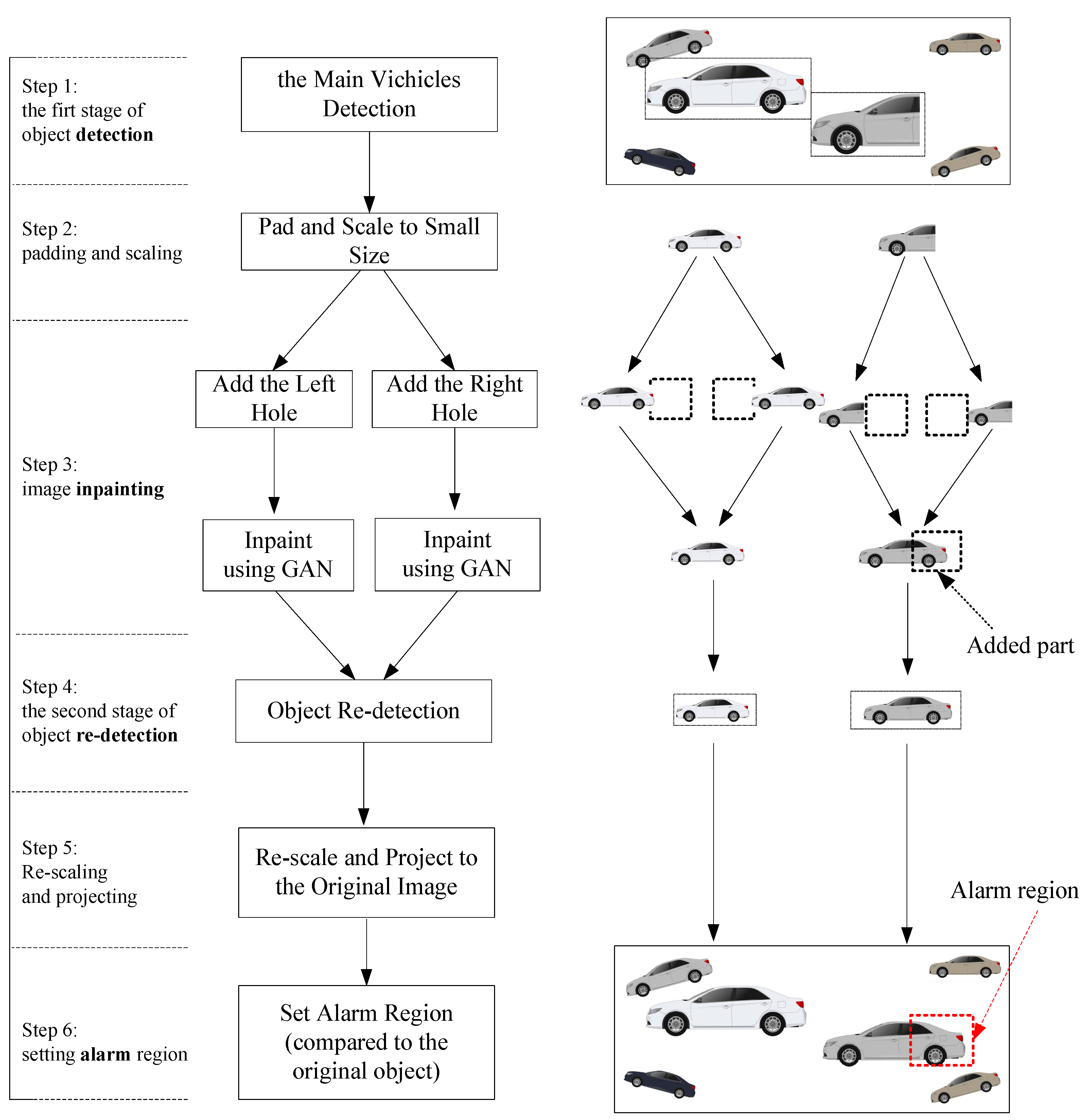
Figure 2 explains the DIDA method in an abstract scenario. The four character “DIDA” comes from the four important steps in the flow chart: object
Detection (step 1),
Inpainting (step 3), object re-
Detection (step 4), and setting
Alarm box (step 6). The single object detection algorithm cannot detect the hidden part, nor can the state of the art algorithms. After the first stage of object detection, the inpainting operation is performed. If the vehicle has a hidden part, the inpainting operation will add a part. Then, the second stage of object detection can detect the entire region including the hidden part.
Step 1 is the first stage of vehicle detection. In the optical system of an autopilot, 24–30 frames are captured in one second. Recently, proposed object detection algorithms have been implemented in real-time detection. To detect the hidden part of the vehicle in this work, the system does not need to detect all vehicles. This is due to two reasons; one is that detecting many objects consumes a great deal of computational resource, and the other is that the small vehicles in view far from the main road do not affect the safe driving. In the top picture of
Figure 2, two major vehicles are detected and marked in rectangles. The left one is a complete vehicle. The right one is incomplete. The right part of the incomplete vehicle cannot be seen because it has the same color as the background. In order to describe the situation visually, the right half of the vehicle merges in the background.
The second step is padding and image scaling. If the shape of the input data is square, the subsequent convolution network should have high performance. For high performance and retaining certain background information, the detected vehicle image is padded from side, upper, and down directions. Padding is detailed in the experiments section. Additionally, high-resolution image inpainting [
32] was proposed, but it uses too many resources. The DIDA focuses on hidden parts and does not need to generate the texture of the original high-resolution image. Therefore, the second step of DIDA reduces the image size after the first stage of object detection. This significantly increases the performance. The scaling operation is both reasonable and necessary.
The third step is image inpainting. The traditional image inpainting methods rely on blurring or copying patches from the side region. It cannot conduct the task of repairing the image to a satisfactory level of completeness. It can only fill the patched holes with part of the background, such as the building, trees, blue sky, white cloud, the road, etc. As of late, image inpainting algorithms based on deep learning have been able to inpaint the hole in a meaningful way. For example, if one eye is covered, the traditional method would fill the covered part with the texture of the skin. The deep learning method, however, would inpaint the covered part with a virtual eye. In the above steps, two major vehicles are detected. One vehicle is complete, while the other only shows half. The latter is dangerous. Autopilot systems cannot judge the actual size of the vehicles only by an optical system. In the DIDA system, all detected vehicles are supposed to be uncompleted. Therefore, the holes that need to be patched are added to the left and right of the object. If the vehicle is complete, the inpainted image fragment should not be part of the vehicle but the background of the scene. In the other case, the inpainted image fragment of the hole should be a part of the vehicle. The inpainting result is shown as the dotted box tagged as “Added part” in step 3 of
Figure 2.
The fourth step is the second stage of object detection. The inpainted images may be the same as the original image or an additional part of the vehicle added to the image. If the detected vehicle image becomes larger than the image before inpainting, this step should find the larger object box. Then, this step outputs a flag that indicates whether or not there is an alarm region.
The fifth step is re-scaling the image to the size of the original image and projecting it to the initial location.
The sixth step is setting the alarm region. If the flag in step 4 is true, we can calculate the alarm region to prevent the vehicle from getting through it.
3.2. The Object Detection about Vehicle
Vehicle detection plays an important role in intelligent transportation and autopilot. Considering the speed and accuracy, we adopt the improved Retina network for object detection. The original Retina Network is a unified network composed of a primary backbone network and two task-specific subnetworks [
2].
The backbone network is utilized to compute a convolutional feature map over an input image. The primary network is based on the Feature Pyramid network [
26] built on the ResNet network [
7].
The first classification subnet predicts the presence probability of an object at each spatial position for each of the anchors and K object classes (K equals 1 here because there is only one vehicle object). It takes an input feature map from the previous primary network’s output. The subnet applies four 3 × 3 convolutional layers, each layer followed by ReLU activations. Finally. sigmoid activations are attached to the outputs. Focal loss is adopted as the loss function.
The second subnet performs bounding box regression. It is similar to the classification network, but the parameters are not shared. This subnet outputs the object’s location as opposed to the anchor box if an object exists. The smooth_L1_loss with sigma that equals three is applied as the loss function to this sub-network.
The focal loss [
2] is designed to address the detection scenario in which there is an imbalance between foreground and background classes. The focal loss is shown as follows:
In Equation (1), gamma is the focusing parameter and alpha is the balancing parameter. The focal loss adds less weight to well classified examples and greater weight to misclassified examples.
To improve the detecting quality and speed, the following adjustments are used. First of all, more training data are added to improve the quality of detection. More vehicle images are extracted from the CompCars dataset [
35], the Stanford Cars dataset [
36], and the pictures captured by our team. It is described in detail in
Section 4. Secondly, the detection threshold is set to 0.8. Thirdly, the class of the detecting object is set to one. Finally, because FPN makes multi-scale predictions, it is not required to detect small objects in this solution. The two minimum layers in the FPN [
26] are deleted.
3.3. Generate Adversarial Network
Recently, the GAN [
11] has been used to generate virtual images. GAN contains two sub-models, the generator model (abbreviated as
G) and the discriminator model (abbreviated as
D).
G generates virtual pictures, which will look like real data. Based on experience, random white noise variable z is defined as the input of
G. Then, function
G(z;
θg) maps the noise variables to the data space. It is represented by a multilayer perceptron with parameters
θg. The sub-model
D is also a multilayer perceptron.
D(
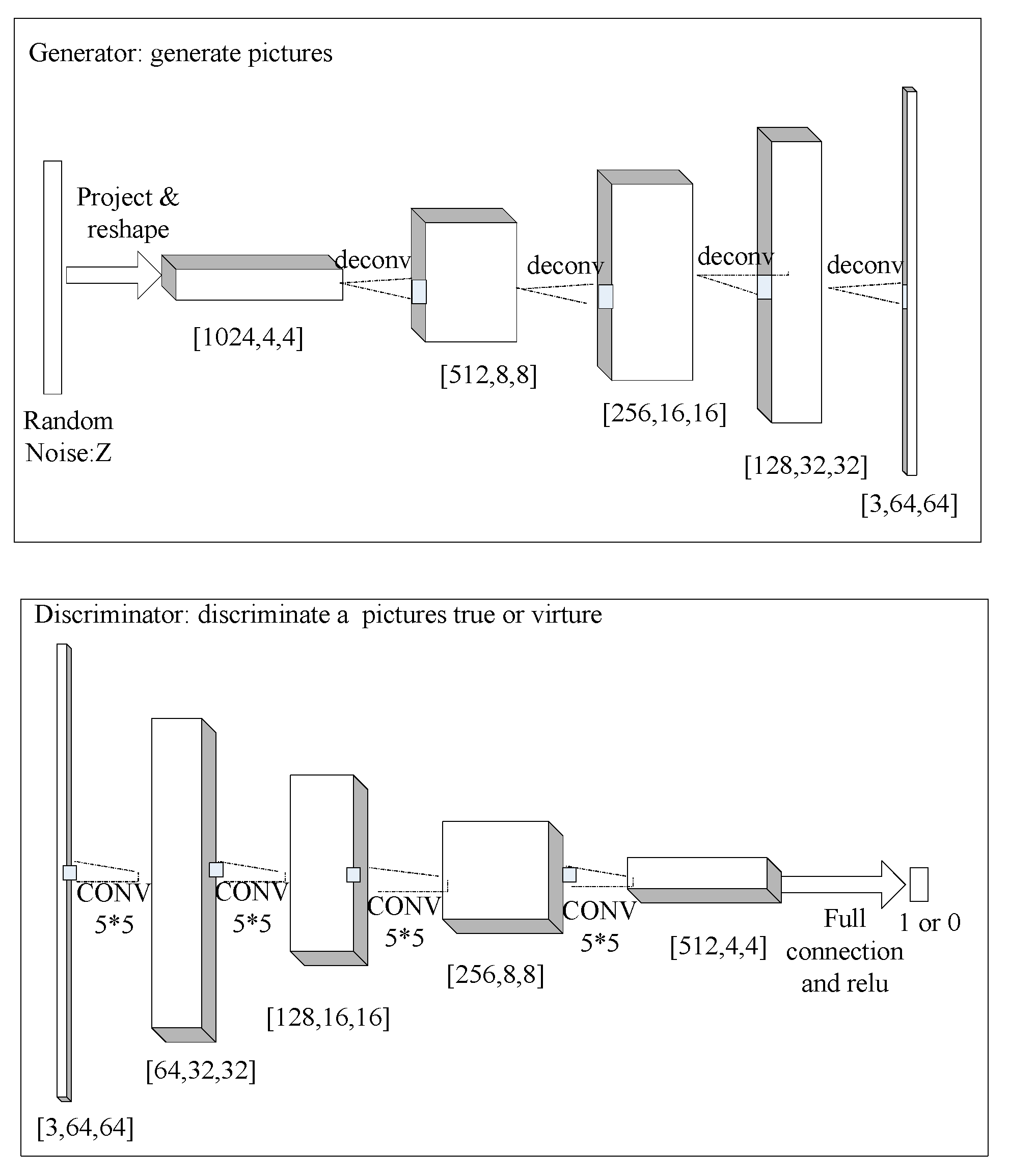
x) represents the probability that the picture x comes from the true data rather than the virtually generated data. The framework of
G and
D is indicated by
Figure 3.
The model
D outputs a Boolean value of one or zero, which respectively indicates real data or virtually generated data if the output data trick the discriminator into thinking the data are real. GAN trains
D to maximize the probability of assigning the correct label to both the true and the virtual data. GAN concurrently trains
G to minimize the same probability. In other words, GANs follow a two-player mini-max optimization process written as formula
. In order to make the calculation easy, the log function is added to
D. Because the input number for log function must be greater than zero, the improved formula of GAN is changed, as shown in Equation (2):
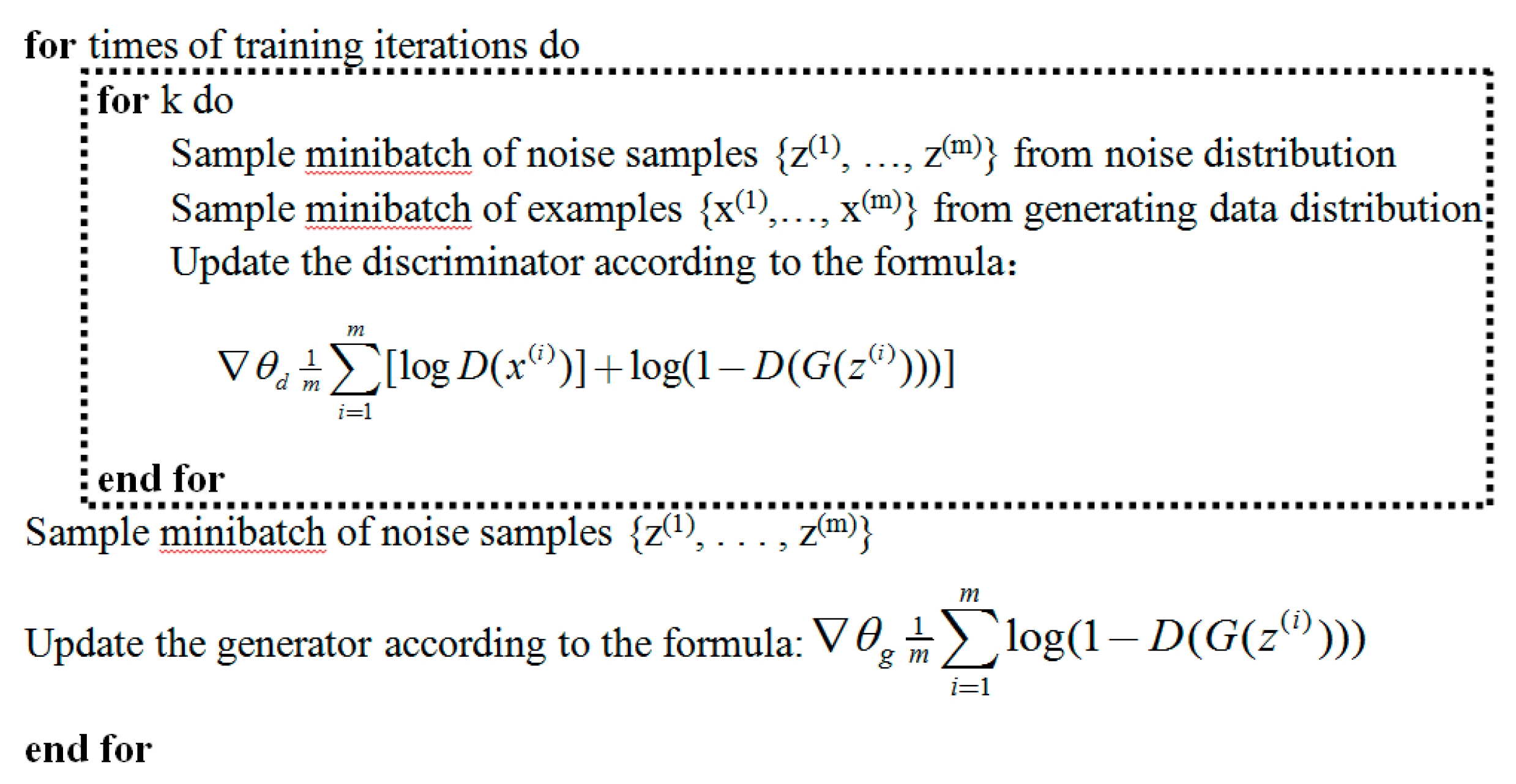
Minibatch stochastic gradient descent [
37] is used in the training stage of GAN. The hyper parameter k is set as two. The k defines the times of the
D for each
G. The algorithm of minibatch stochastic gradient descent in the experiment is shown as
Figure 4.
The pseudo-code surrounded by the dotted rectangle achieves the optimization of the D. All of the code completes synchronal optimization of the G and D. If the various pictures are all trained at the same time, the diversity of the image class results in chaotic and meaningless virtual images. If there are numerous kinds of images, the generating process should be done category by category. In this case, only one image category (vehicle) is used.
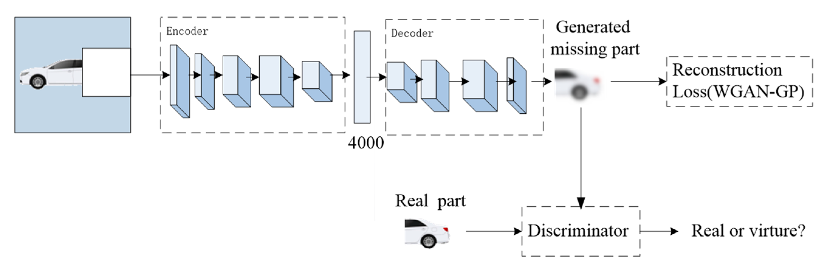
3.4. The Framework of Image Inpainting
The architecture of the image inpainting to predict missing parts from their surroundings is shown in
Figure 5.
Figure 5 shows the process of inpainting the right predicting region in the white box. The upper half of the figure describes the process of generating the virtue image using the auto-encoding structure [
38]. The rest of the figure describes the decision process by the discriminator of GAN.
Encoder: The encoder is derived from the AlexNet architecture [
4]. Given an input image with a size of 128 × 128, we use five convolutional layers ([64,4,4], [64,4,4], [128,4,4], [256,4,4], [512,4,4]) and the following pooling layer to compute an abstract [512,4,4] dimensional feature representation. In contrast to AlexNet, our model is not trained for ImageNet classification but for predicting the missing hole.
The layer between the encoder and the decoder is a channel-wise fully-connected layer [
30]. This layer is designed to propagate information within each feature map. If the dimension of the input layer is [m, n, n], this layer outputs the same size feature maps.
Decoder: The decoder generates the virtue image with the missing region using the features of the encoder output. The decoder contains a series of up-convolutional layers ([512,4,4], [256,4,4], [128,4,4], [64,4,4], [64,4,4]) [
8,
39,
40] and ELUs activation function [
41]. An up-convolutional is utilized to result in a higher resolution image. The idea behind the decoder is that the series of up-convolutions and nonlinear activation function comprises a non-linear up-sampling of the feature produced by the encoder.
Joint Loss Function: The reconstruction loss function is set as the following joint loss function:
Given the input image
x0, we would like to find the unknown output image
x.
R is used to denote the missing hole region in
x. The function
h(·) defines the operation of extracting a sub-image or sub-feature-map in a rectangular region, i.e.,
h(
x,
R) returns the color content of
x in
R. The term
represents the total variation regularization to smooth the image:
Empirically,
is set as 5 × 10
−6 to balance the two losses. In this loss Equation (4), the texture loss is not adopted because each texture process should consume more than eight seconds [
32].
Discriminator: The structure of the discriminator is the same as in
Figure 2. It decides whether an image is true or not.
4. Experiments and Results
This section first presents the datasets, then real world vehicle detection and inpainting are demonstrated to show the hidden part of a vehicle.
4.1. Datasets
One of the reasons for the great progress in deep learning is big data. The proposed approach is based on deep learning, thus sufficient valid data are also essential for this approach to function correctly. We prepared the following datasets.
The Comprehensive Cars (CompCars) dataset [
35] contains data from two scenarios, web-based and surveillance-based. The web-based data contain 136,726 images capturing entire car sets and images capturing the car parts. The surveillance-based data contain car images captured in the front view. In this work, only cars from the web-based set are used. The Stanford Cars dataset [
36] contains 16,185 images of 196 classes of cars. The data are divided into 8144 training images and 8041 testing images. This work uses both training and testing images as training data. However, the aforementioned car datasets do not have enough vehicle images captured from the sides. Therefore, our team took about 50,000 vehicle pictures. These pictures were collected from the sides of the cars beside the busiest crossroad, the ancient Bell Town and Drum Town, in Xi’an, China. The new dataset was created and called the Complex Traffic Environment (CTE-Cars). The training dataset used in this work is a combination of the CompCars dataset, the Stanford Cars dataset, and CTE-Cars.
4.2. The First Stage of Object Detection (Step 1)
The test dataset contains pictures taken in a new scene. They do not belong to the training dataset. In this way, the set of the experiments ensures the validity of the test results and avoids overfitting.
The focal loss [
2] is applied to all anchors [
19] in each picture during the training process. The total focal loss of a picture is calculated as the sum of the focal loss over all anchors. It is normalized by the amount of anchors assigned to a ground-truth box. In general, alpha should be decreased slightly while gamma is increased in Equation (1). In the experiment, the experimental parameters gamma: 2 and alpha: 0.25 work best. The primary network of the model is ResNet-50 [
7]. In the model, weight decay is set to 0.0001, momentum is set to 0.9, and initial learning rate is set to 0.01 during the first 60,000 iterations. Learning rate is reduced by 10% after every 60,000 iterations.
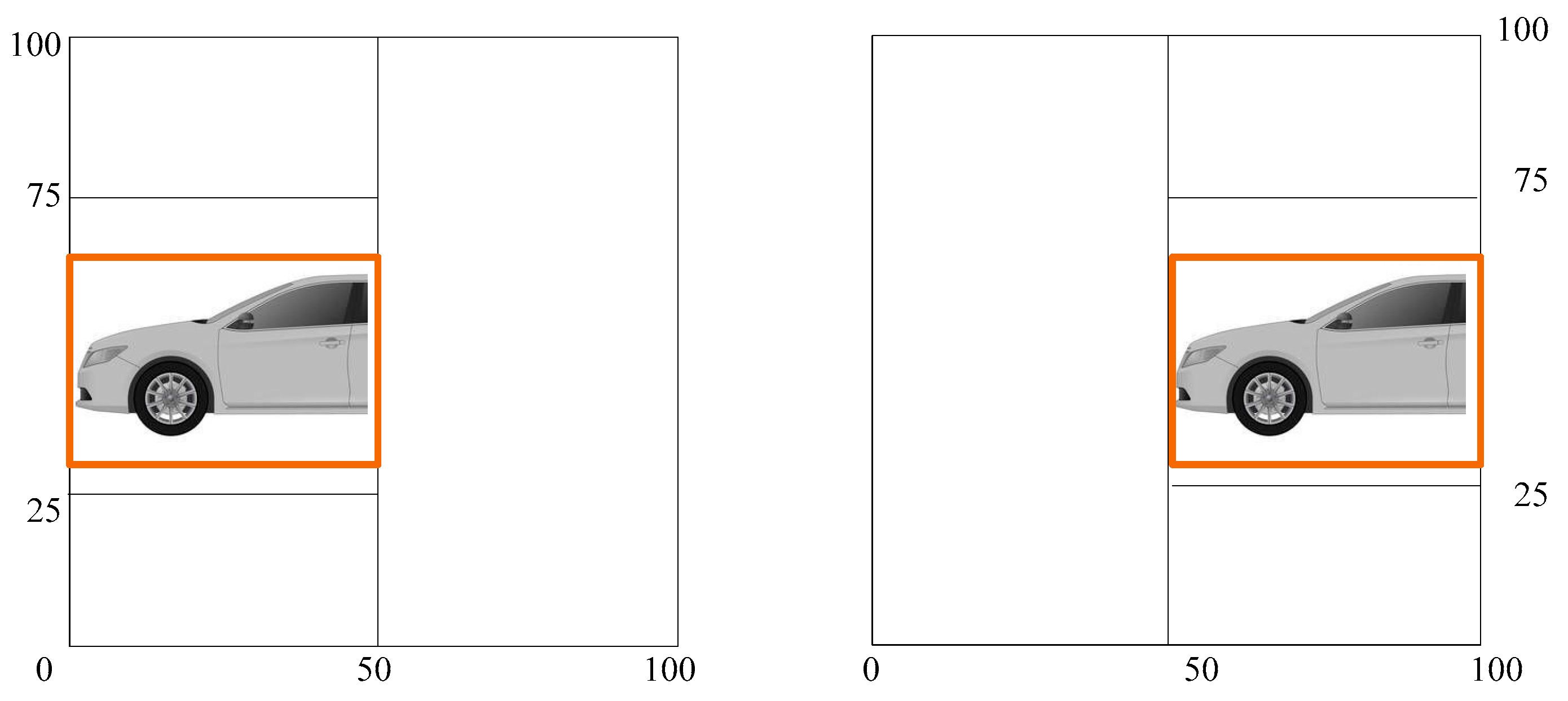
The next step is padding and scaling the picture size.
The orange box is the region of the detected vehicle. A right padding is to extend the right part and form a square image, as shown in the left sub-graph of
Figure 6. A left padding is to extend the left part and form a square image, as shown in the right sub-graph of
Figure 6. At this stage, the images are padded to form the complete image.
The purpose of the paper is to obtain information about a certain dangerous area to avoid accidents, not to precisely repair the appearance of the vehicle. To speed up the calculation, the detection image is scaled down to a square of 128 × 128 pixels. Then, the small images are imported to the network.
4.3. Image Inpainting and Re-Detection (Step 3 and Step 4)
Table 1 shows the flow chart from the padding to re-detection. Because the state of the art object detection algorithms cannot detect the vehicle with hidden parts, as shown in
Figure 1, we do not compare with other object detection algorithms in this section. Pictures in the first row are the padded images, which are very clear. However, the pictures in the second row are blurrier than the pictures in the first line because they are scaled down to 128 × 128 pixels. Row 3 shows the images after inpainting. The left and right inpainting are mandatory whether there are hidden parts or not. Object re-detection is shown in row 4. This is the fourth step of DIDA. If a vehicle has a hidden part, the detected region in the second stage of object detection should be bigger than the region of the first stage of detection. This is shown in the orange box in column 3 of rows 4 and 2. Otherwise, the two regions should be same, as shown in column 4 of rows 4 and 2.
The images from the rows 5 to 8 show the inpainting results of the traditional methods. The methods are the texture synthesis method based on the algorithm [
42] (row 5), Absolute Minimizing Lipschitz Extension (AMLE) [
43] (row 6), Mumford-Shah Inpainting with Ambrosio-Tortorelli approximation [
44] (row 7), and Transport Inpainting [
45]. None of the traditional methods could handle the large region inpainting.
In the test phase, we randomly select 200 vehicle pictures to be used. The test dataset includes two types of pictures with and without hidden parts. In the real world, it is difficult to find the vehicle picture with a hidden part to verify the correctness of this algorithm. The test picture with a hidden part is a virtual picture created by Photoshop. No test pictures are seen by the train model. They are divided into two categories, each of which has 100 pictures. In the first category of the test dataset, the test pictures have a one quarter hidden region. In the second category of the test dataset, the test pictures have a half hidden region.
There are four different qualitative results of the algorithm—adding a part to the complete vehicle (wrong), adding a part to the incomplete vehicle (right), adding nothing to the complete one (right), and adding nothing to the incomplete one (wrong). In the research, we quantitatively define a correct result if the difference of the area between the predicted vehicle and the grand-truth is less than 10%. The precision results of the two test datasets were 91% and 82%, respectively.
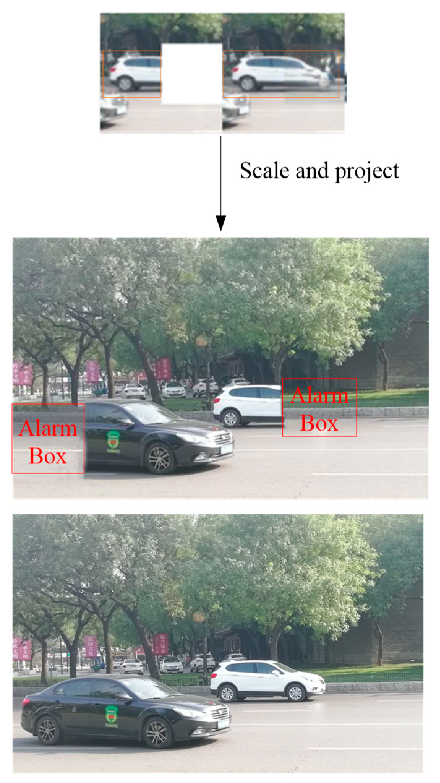
4.4. Re-Scaling, Projecting (Step 5), and Setting Alarm Region (Step 6)
The left orange box in the top of
Figure 7 shows the detected region of the vehicle before inpainting. The right orange box is the re-detected vehicle region after inpainting. The latter is bigger than the former. The difference between the two boxes is the hidden part. The vehicles are projected to the original image. The red box, the projected difference region, is defined as the alarm region (alarm box). Although the alarm area cannot be recognized as a part of the vehicle by a general vision system, this area is still dangerous.
Figure 7 omits the procedure of the black car. The bottom picture is the ground-truth image.
This algorithm does not lead to any risk. The DIDA algorithm performs an “adding” action based on the original vehicle image, not a “deleting” action. The worst scenario is that a part is added to a complete vehicle, which only reduces traffic efficiency.
5. Discussion
In uncommon situations, the color of a part of a vehicle is similar to the background color, which results in an error of optical object detection and consequently causes a failure of autopilot. The error can even cause a traffic accident. The proposed DIDA method solves this problem. As far as we know, the work is the first attempt to solve the problem by combining the object detection and image inpainting. However, the method has many steps, and the speed of the whole process needs improvement in the future. YOLOv3 [
46] should be tested to improve the speed in the future.
In addition, the repaired parts are not perfect, such as the lack of tires. Although this does not affect the task, the improved GAN algorithm can be used in the future to generate the hidden part more accurately.
The category of the test pictures is not enough. In this research, only the normal condition of the test environment is considered. In the future, test pictures with sufficiently high numbers of vehicle categories should be added, such as different distances, different lighting conditions, angles of sunshine, shadows and background, etc.
In this work, we demonstrate an imaginative inpainting of a vehicle. It embodies a higher level artificial intelligence, such as prediction and imagination. The idea and method can be extended to other areas, such as underwater detection, intelligent transportation, robotics, etc.
Moreover, we share the CTE-Cars dataset that can be used for other future research of autopilot.


