Weighted Neighborhood Preserving Ensemble Embedding

Abstract

Neighborhood preserving embedding (NPE) is a classical and very promising supervised dimensional reduction (DR) technique based on a linear graph, which preserves the local neighborhood relations of the data points. However, NPE uses the K nearest neighbor (KNN) criteria for constructing an adjacent graph which makes it more sensitive to neighborhood size. In this article, we propose a novel DR method called weighted neighborhood preserving ensemble embedding (WNPEE). Unlike NPE, the proposed WNPEE constructs an ensemble of adjacent graphs with the number of nearest neighbors varying. With this graph ensemble building, WNPEE can obtain the low-dimensional projections with optimal embedded graph pursuing in a joint optimization manner. WNPEE can be applied in many machine learning fields, such as object recognition, data classification, signal processing, text categorization, and various deep learning tasks. Extensive experiments on Olivetti Research Laboratory (ORL), Georgia Tech, Carnegie Mellon University-Pose and Illumination Images (CMU PIE) and Yale, four face databases demonstrate that WNPEE achieves a competitive and better recognition rate than NPE and other comparative DR methods. Additionally, the proposed WNPEE achieves much lower sensitivity to the neighborhood size parameter as compared to the traditional NPE method while preserving more of the local manifold structure of the high-dimensional data.

1. Introduction

In many machine learning applications, such as data classification [1,2], face recognition [3,4], signal processing [5,6], and text categorization [7,8], the input data is usually high-dimensional which makes the calculations too complex, as well as requiring more computational time. In order to boost the performance and computational efficiency, various dimensionality reduction (DR) techniques have been proposed to preprocess these high-dimensional data. The employment of DR techniques aims at extracting the optimal representative features and transforming the original high-dimensional data into a low-dimensional feature space using different algorithms. According to the general framework these DR methods can be grouped into linear and non-linear methods [9].

Principal component analysis (PCA) [10] and linear discriminant analysis (LDA) [11] are two well-known linear subspace learning DR approaches. Both PCA and LDA assumes that the sample lies on a linear embedded manifold. PCA preserves the global geometrical information whereas LDA tries to preserve the global discriminant information of the high-dimensional data points. As these both aforementioned linear methods are very simple and convenient to use, they still fail to exploit the essential non-linear structure of the data. In order to overcome the issues in linear DR methods, many manifold learning algorithms have been introduced to discover the non-linear structure of the data. These include isometric feature mapping [12], local linear embedding (LLE) [13], and Laplacian eigenmaps (LE) [14]. However, these algorithms suffer from the out-of-sample problem [15].

To solve the out-of-sample problem in manifold learning algorithms, graph-based embedding methods have been presented to reveal the local manifold structure of the data [16]. Graph-based embedding models preserve the spatial similarities of neighborhoods of the original data points in the form of node pairs by defining each node of graph as a low-dimensional eigenvector using a graph similarity weight matrix. Finally, the optimized projections can be computed by solving the graph-based eigenvector decomposition. Locality preserving projection (LPP) [17] and neighborhood preserving embedding (NPE) [18] are famous graph-based embedding manifold learning DR techniques. Both methods preserve the intrinsic manifold structure of the data without particular conjecture of the data distribution.

Due to the simplicity and effectiveness, NPE has been investigated in many recent studies [19,20,21,22]. Although NPE has shown better results than other competitive DR algorithms it is still highly sensitive to the neighborhood size parameter [23,24] as it uses the K nearest neighbor (KNN) criteria for constructing an adjacency graph. In this paper, we propose a novel DR method called weighted neighborhood preserving ensemble embedding (WNPEE). With this approach, our method can preserve more satisfactory local neighborhood structure that illustrates the intrinsic manifold of original high-dimensional data. The key properties of the proposed WNPEE method are summarized below:

• Unlike NPE, the proposed WNPEE constructs an ensemble of adjacent graphs with the number of nearest neighbors varying. With this graph ensemble building, WNPEE can obtain the low-dimensional projections with optimal embedded graphs pursuing in a joint optimization way.
• As rationale behind proposed WNPEE algorithm is similar to NPE; therefore, NPE can be viewed as a special instance of the WNPEE for a fixed parameter of the neighborhood size.
• The WNPEE provides an efficient weighting scheme for the eigenspace which makes it much less sensitive to the parameter of neighborhood size and it can get more stable recognition rate as compared to NPE.

We arrange rest of the paper, subsequent to introduction in Section 1 in the following manner. In Section 2, we present a brief but comprehensive review of state-of-the-art DR methods. The preliminaries of both LPP and NPE are given in Section 3. In Section 4, we describe the proposed WNPEE method with suitable explanation. Experimental results with a comparative discussion of the proposed method along with four comparative DR methods are shown in Section 5. We draw our conclusion and the future directions of research in Section 6.

2. Related Work

Recently, a number of dimensionality reduction methods have been developed with different ideas and methodology. However the aim of these numerous methods is same, that is, to obtain low-dimensional data on which further machine learning tasks can be easily performed with improved computational complexity. The following are some related comparable linear DR techniques used in this article to show the superiority of the proposed WNPEE method.

Linear dimensionality reduction approaches are widely used in face recognition because of their relative simplicity, analytical manipulability, and the direct ability to deal with the testing data points. The most popular linear DR methods include PCA [10], LPP [16], LDA [12], and NPE [18]. In face recognition applications, they are well known as Eigenfaces [11], Fisherfaces [16], Laplacianfaces [25], and NPEfaces [18]. Eigenfaces, which is based on PCA, finds a set of mutually orthogonal basis vectors to characterize the high-dimensional data in a least-squares sense. Different from Eigenfaces, which does not appropriately use label information of the given input data, Fisherfaces spread on LDA to search the information on which the data points belonging to different classes are expected as distant from each other as possible. However, it assumes that the data points of the same class must be close to each other. Therefore, Laplacianfaces was proposed to find an optimally linear approximation of the eigenfunctions using the Laplace Beltrami operator on the face manifold [25]. The representation map generated by LPP preserves better local information of the essential manifold structure with more discriminating power.

Additionally, to preserve the neighborhood relations of high-dimensional data an unsupervised locally linear embedding (LLE) was firstly introduced by Roweis and Saul [13]. It is based on two linear perceptions: first is that each data point and its neighbors lies on or close to a locally linear cover of a manifold, and second is that the local symmetrical classification in original data space is unchanged in the output data space. LLE is very effective for feature extraction of high-dimensional data, yet it is unable to generate a loading matrix necessary for construction of a prediction model. Therefore, to overcome this problem a linear approximation of the LLE algorithm called neighborhood preserving embedding (NPE) has been developed [18]. NPE possibly outperforms Eigenfaces and Fisherfaces to preserve more Euclidian structure in DR tasks. The following is a brief overview of these related linear dimensionality reduction algorithms.

Let us consider $P={\{p_i\in {ℝ}^D\}}_{i=1}^N$ a high $D$-dimensional data with $N$ number of samples. Linear DR mapping is to assign the original high-dimensional data to a low $d$-dimensional data i.e., $Q={\{q_i\in {ℝ}^d\}}_{i=1}^N$ $\left(d\ll D\right)$. If $A$ is a transformation matrix, then linear DR is defined as:

$$q_i=A^T{p}_i for i=1,\dots , N.$$

(1)

PCA idea is to find a projection direction that will give maximum variance, i.e., the reconstruction error can be minimal. The objective function of PCA is defined as follows:

$$A_{opt}=\arg ma{x}_A{\displaystyle \sum }_{i=1}^N{(q_i-\overline{q})}^2,―$$

$$A_{opt}=\arg ma{x}_A{A}^{T}CA.$$

(2)

where $\overline{q}=\frac{1}{N}{{\displaystyle \sum }}^{}{q}_i$ and $C$ is the data covariance matrix. Finally the eigenvalues and orthogonal set of eigenvectors are computed for this covariance matrix. However, PCA impairs class discrimination as it uses directions which are only efficient for class representation. Thus, LDA, a linear supervised DR method, is a better choice for extracting discriminant features. Let the input data $P$ belong to $l$ classes, then LDA is optimized by the followig objective function:

$$A_{opt}= \arg ma{x}_A\frac{A^T{S}_{B}A}{A^T{S}_{W}A},$$

(3)

$$S_B={\displaystyle \sum }_{i=1}^l{N}_i\left(m^{\left(i\right)}-m\right){(m^{\left(i\right)}-m)}^T,―$$

(4)

$$S_W={\displaystyle \sum }_{i=1}^l\left({\displaystyle \sum }_{j=1}^{N_i}\left(p_j^{\left(i\right)}-m^{\left(i\right)}\right){(p_j^{\left(i\right)}-m^{\left(i\right)})}^T\right)―$$

(5)

where $m$ is the total sample mean vector, $N_i$ is the number of samples in the $i$th class, $m^{\left(i\right)}$ is the average vector ofthe $i$th class, and $p_j^{\left(i\right)}$ is the $j$th sample in the $i$th class. Additionally, $S_B$ is the between-class scatter matrix and $S_W$ is the within-class scatter matrix.

3. Preliminaries

In this section we briefly describe the functioning of LPP and NPE DR algorithms.

3.1. Locality Preserving Projections

LPP is an unsupervised graph-based embedding method [17]. LPP is designed with different objective principle from classical linear DR techniques. Due to locality preserving quality of LPP, it has been used in many information retrieval applications [26,27,28]. LPP can be simply functional everywhere unlike non-linear DR techniques. LPP could be carry out in the inventive space or in the reproducing kernel Hilbert space into which data points are mapped. The functioning of the LPP is defined as follows:

• Constructing an adjacent graph: using $\mathsf{\epsilon }$-neighborhood or $k$-neighborhood. In the ε-neighborhood: nodes $i$ and $j$ are connected by an edge if ${||p_i-p_j||}^2< \epsilon$. In the $k$-neighborhood: nodes $i$ and $j$ are connected by an edge if $i$ is in $k$ nearest neighbors of $j$ or $j$ is in $k$ nearest neighbors of $i$.
• Choosing the weights: Weights $W_{ij}$ are given to edges between nodes $i$ and $j$ by a symmetric weight matrix $W$, computed either by uniform weight or Gaussian weight of Euclidean distance.$W$ is often defined as:

  $$W_{ij}=\{\begin{array}{cc}\hfill \frac{exp{||p_i-p_j||}^2}{t},& p_j\in \mathrm{KNN} of p_i or p_i\in \mathrm{KNN} of p_j\\ \hfill 0,& otherwise.\end{array},$$

  (6)

  where parameter $t$ is a positive constant.
• Eigenmaps: by computing eigenvectors and eigenvalues for the below eigenvector problem:

  $$PL{P}^{T}a=\lambda PD{P}^{T}a.$$

  (7)

  where $D$ is a diagonal matrix whose entities are column (or row) sum of $W$, $D_{ii}={\displaystyle \sum }_j{W}_{ij}$, $L=D-W$ is the Laplacian matrix and $a$ is a transformation vector.

3.2. Neighborhood Preserving Embedding

The neighborhood preserving embedding (NPE) method is identical to LPP as both are targeted to discover the local structure of the original data manifold, yet their objective functions are totally different [19]. Linearity makes NPE a fast and suitable technique for practical applications [29,30,31,32,33,34,35,36]. NPE can be performed in either supervised or unsupervised mode. When the class information is available, it can be utilized to build a better weight matrix. It models the manifold structure directly by constructing the nearest-neighbor (NN) graph that reveals neighborhood relations of data points, and then retains the graph structure in the projection. The algorithmic procedure of NPE is defined as follows:

• Constructing an adjacency graph: using $k$-neighborhood or $\epsilon$-neighborhood. In the $k$-neighborhood: a directed edge from nodes $i$ and $j$ if $p_j$ is in $k$ nearest neighbors of $p_i$. In the $\epsilon$-neighborhood: put an edge between nodes $i$ and $j$ if ${||p_i-p_j||}^2\le \epsilon$.
• Computing the weights: Weights $W_{ij}$ are given to edges between nodes $i$ and $j$ by a symmetric weight matrix $W$, and weight 0 if there is no such edge. The weight is calculated by minimizing following objective function:

  $$\min {\displaystyle \sum }_i{||p_i-{\displaystyle \sum }_j{W}_{ij}{p}_j||}^2,$$

  (8)

  $$s.t{\displaystyle \sum }_j{W}_{ij}=1 , j=1,2,\dots N.$$
• Computing the projections: final projections are obtained by minimizing the following eigenvector problem:

  $$PM{P}^{T}a=\lambda PD{P}^{T}a.$$

  (9)

  where $M={\left(I-W\right)}^T\left(I-W\right)$, $I$ is an identity matrix and $D$ is a diagonal matrix as in Equation (7). The optimal mapping transformation matrix $A$ is embedded by the optimal mapping transformation vectors $\left(a_0, a_1,\dots ,a_{d-1}\right)$, which are arranged in the order of their corresponding eigenvalues as ${\lambda }_0\le \dots \le {\lambda }_{d-1}$.

4. The Proposed WNPEE Method

The aforementioned NPE is based on graph embedding and the neighbor relationship is measured by an artificially-constructed adjacent graph. Usually the KNN [2] criteria is used to construct an adjacent graph which makes the performance of the NPE very sensitive to the parameter of the neighborhood size. Thus, to overcome the neighborhood size sensitivity in NPE, we are motivated to propose a novel DR technique called weighted neighborhood preserving ensemble embedding (WNPEE). The proposed WNPEE is designed to capture the locality of the original data in the phase of manifold learning using an ensemble of adjacent graphs with varying the number of nearest neighbors. This graph ensemble building helps in obtaining the optimal embedded graph with low-dimensional projections pursued in a joint optimization way. Simultaneously, WNPEE makes the projections less sensitive to the parameter of the neighborhood size.

Let us assume a high-dimensional data set $X={\{x_i\in {ℝ}^D\}}_{i=1}^N$, where $x_i$ are data samples, $D$ represents the dimensions, and $N$ is the total number of samples. WNPEE aims to reduce the original $D$-dimensional data into reduced $d$-dimensional data $\left(d\ll D\right)$ by constructing an optimal transformation matrix $A$. Let $Y={\{y_i\in {ℝ}^d\}}_{i=1}^N$ represent the reduced $d$-dimensional data such that $A$ maps $x_i$ to $y_i$ or we can say $y_i$ represents $x_i$, where $y_i=A^T{x}_i$ in which locality of $x_i$ is preserved by linear dimensionality reduction. In our proposed WNPEE method, the low-dimensional projections are carried out through the following steps:

Step 1: Firstly, it constructs an ensemble of adjacent graphs unlike NPE, i.e., constructing only one graph. Let $G_1, G_2,\dots , G_L$ are adjacent graphs computed by varying the neighborhood size parameter ranges from $1 to L$. These graphs can be formed either by $\mathrm{K}$ nearest neighbors $\left(\mathrm{KNN}\right)$ or $\mathsf{\epsilon }$-neighborhood. In proposed WNPEE, we assume the $\mathrm{KNN}$ criteria for constructing an ensemble of adjacent graphs. Each adjacent graph having $N$ nodes, where the $i$-th node is corresponds to data point $x_i$. Using the $\mathrm{KNN}$ method, a directed edge is placed from node $i$ to node $j$ if $x_j$ is among $K$ nearest neighbors of $x_i$. Simultaneously weights are given to multiple adjacent graphs to ensemble them, by using parameter ${\alpha }_k$ where $k$ is the neighborhood size parameter.

Step 2: Secondly, we compute the weights on the edges with fixed parameter ${\alpha }_k$ where the neighborhood size $k=1 to L$. By using a fixed ${\alpha }_k$ we assume that each adjacent graph has an equal weight, i.e., if $L=10$ then each adjacent graph have weight $1/10$ while computing the weights on the edges. Let ${\mathrm{W}}_{\mathrm{k}}$ be an $N\times N$ weight matrix for every $k$ adjacent graph, with $W_{k,ij}$ is the weight of the edge from node $i$ to $j$, and 0 if there is no such edge. Minimization of the below objective function is used for weighting the edges:

$$\min {\displaystyle \sum }_i||x_i-{\displaystyle \sum }_j{\displaystyle \sum }_k{\mathsf{\alpha }}_k{W}_{k,ij}{x}_j||{}^2,$$

$$s.t{\displaystyle \sum }_j{W}_{k,ij}=1,\hspace{1em}\hspace{1em}j=1,2,\dots ,N.$$

(10)

Step 3: Then the low-dimensional projections are obtained by solving the below generalized eigenvalue problem:

$$XM{X}^{T}a=\lambda X{X}^{T}a.$$

(11)

where $X$ is high-dimensional data,$M={\left(\mathrm{I}-{{\displaystyle \sum }}^{}{\alpha }_k{\mathrm{W}}_{\mathrm{k}}\right)}^T\left(\mathrm{I}-{{\displaystyle \sum }}^{}{\alpha }_k{\mathrm{W}}_{\mathrm{k}}\right)$, and $I=diag\left(1,\dots ,1\right)$ is a diagonal matrix. By solving Equation (11), the low-dimensional projection vectors $a_0, a_1,\dots ,a_{d-1}$ are obtained with their corresponding eigenvalues ${\lambda }_0\le \dots \le {\lambda }_{d-1}$. Thus, WNPEE embedding is as follows:

$$x_i\to y_i= A^T{x}_i, A=(a_0, a_1,\dots ,a_{d-1}).$$

(12)

where $y_i$ is a $d$-dimension vector and $A$ is a $D\times \mathrm{d}$ matrix.

Step 4: Finally, we compute the weight coefficients ${\alpha }_1,{\alpha }_2,\dots ,{\alpha }_L$ according to Equation (26), on $G_1, G_2,\dots , G_L$ adjacent graphs while taking the projection vector $a$ fixed obtained from Equation (11). With these updated weights on ensemble adjacent graphs, the weighted neighborhood preserving ensemble embedding projection vector $a$ as well as ${\alpha }_k$ are iteratively computed until the loss converges. The whole WNPEE procedure is summarized in Algorithm 1.

Algorithm 1. The weighted neighborhood preserving ensemble embedding algorithm.

Input: High-dimensional data $X$ Output: projection vector $a$ Parameter: ${\alpha }_k$ Initialize: - Construct an ensemble of adjacent graphs using $KNN$ with ${\alpha }_k$ weights while loss not converged do 1. Computing the weights on edges with fix ${\alpha }_k$ acc. to (10) 2. Obtain projection vector $a$ acc. to (11) 3. Fix $a$ and update ${\alpha }_k$ acc.to (26) 4. Compute current loss End while

Obtaining Parameter ${\alpha }_k$ in the Proposed WNPEE

In this paper we proposed an approach to make NPE less sensitive to neighborhood size $k$ while preserving the local manifold structure of the input data during dimensionality reduction. To do so we introduce a new ensemble of adjacent graphs framework to NPE manifold learning technique. We therefore discuss how to obtain the value for the parameter ${\mathsf{\alpha }}_{\mathrm{k}}$, which is the weight coefficient for the ensemble adjacent graphs which satisfies ${\mathsf{\alpha }}_{\mathrm{k}}\ge 0$ and ${\displaystyle \sum }_{k=1}^L{\alpha }_k=1$.

In WNPEE each node of the adjacent graph can be represented by a linear combination of its neighbors with the weight $W_{k,ij}$ on the edge. Thus, the local spatial distribution of these patches can be characterized by linear coefficients that reconstruct each data point from its neighbors. With proper constraints and fixed $W_{k,ij}$ weights [18], the reconstruction errors are measured by the following cost function:

$$\Phi \left(y\right)= {\displaystyle \sum }_i{\left(y_i-{\displaystyle \sum }_j{\displaystyle \sum }_k{\alpha }_k{W}_{k,ij}{y}_j\right)}^2.$$

(13)

Although the projections are linear, i.e., $y^T=a^{T}X$, where the $i$-th column vector of $X$ is $x_i$ it can be written as:

$$z_i=y_i-{\displaystyle \sum }_j{\displaystyle \sum }_k{\alpha }_k{W}_{k,ij}{y}_{j },$$

(14)

or in vector form:

$$z=y-{{\displaystyle \sum }}^{}{\alpha }_k{\mathrm{W}}_{\mathrm{k}}y,$$

(15)

$$z=\left(\mathrm{I}-{{\displaystyle \sum }}^{}{\alpha }_k{\mathrm{W}}_{\mathrm{k}}\right)y.$$

(16)

where $I$ is a identity matrix. Further the cost function can be reduced to:

$$\Phi \left(y\right)= {\displaystyle \sum }_i{\left(z_i\right)}^2,$$

(17)

$$\Phi \left(y\right)= z^{T}z,$$

(18)

$$\Phi \left(y\right)=y^T{\left(\mathrm{I}-{{\displaystyle \sum }}^{}{\alpha }_k{\mathrm{W}}_{\mathrm{k}}\right)}^T\left(\mathrm{I}-{{\displaystyle \sum }}^{}{\alpha }_k{\mathrm{W}}_{\mathrm{k}}\right)y,$$

(19)

$$\Phi \left(y\right)=a^{T}X{\left(\mathrm{I}-{{\displaystyle \sum }}^{}{\alpha }_k{\mathrm{W}}_{\mathrm{k}}\right)}^T\left(\mathrm{I}-{{\displaystyle \sum }}^{}{\alpha }_k{\mathrm{W}}_{\mathrm{k}}\right)X^{T}a,$$

$$s.t. {\displaystyle \sum }_{k=1}^L{\alpha }_k=1.$$

(20)

However from Equation (20), we can see that $\Phi \left(y\right)$ is linear with respect to ${\alpha }_k$. It is also noted that the optimal solution of the linear programming will always be the extreme points, that is either ${\alpha }_k$= 0 or ${\alpha }_k$ = 1, which means there will only be one adjacent graph selected contrary to our objective of exploring the rich complementation of multiple adjacent graphs. Thus, to overcome this problem, we make a relaxation by considering ${\alpha }_k$ to be ${\alpha }_k^r$(r represents a control parameter for the weights of the multiple adjacent graphs). Thus, while $r>1$ the outcome is a balance of multiple adjacent graphs [37,38]. Thus, by adding a Lagrangian multiplier, we obtain the formulation of WNPEE as:

$$ℒ\left(y,\lambda \right)=a^{T}X{\left(\mathrm{I}-{{\displaystyle \sum }}^{}{\alpha }_k^r{\mathrm{W}}_k\right)}^T\left(\mathrm{I}-{{\displaystyle \sum }}^{}{\alpha }_k^r{\mathrm{W}}_k\right)X^{T}a-\lambda \left({{\displaystyle \sum }}^{}{\alpha }_k^r-1\right).$$

(21)

Let $B=\left(\mathrm{I}-{{\displaystyle \sum }}^{}{\alpha }_k^r{\mathrm{W}}_k\right)$, and taking partial derivative by using Leibniz’s notation as follows:

$$\frac{\partial ℒ\left(y,\lambda \right)}{\partial \left({\alpha }_k\right)}= \frac{\partial \left(\Phi \left(y\right)\right)}{\partial \left(B\right)}\frac{\partial \left(B\right)}{\partial \left({\alpha }_k\right)},$$

(22)

$$\frac{\partial ℒ\left(y,\lambda \right)}{\partial \left(B\right)}=2 tr\left[\left(\mathrm{I}-{{\displaystyle \sum }}^{}{\alpha }_k^r{\mathrm{W}}_k\right)X^T\mathit{a} {\mathit{a}}^{T}X\right],$$

(23)

$$\frac{\partial \left(B\right)}{\partial \left({\alpha }_k\right)}= -tr \left({\mathrm{W}}_{\mathrm{k}}\right)r {\alpha }_k^{r-1},$$

(24)

Therefore:

$$\frac{\partial ℒ\left(y,\lambda \right)}{\partial \left({\alpha }_k\right)}=r {\alpha }_k^{r-1} tr \left\{\left[\left(\mathrm{I}-{{\displaystyle \sum }}^{}{\alpha }_k^r{\mathrm{W}}_k\right) X^{T}a a^{T}X\right]{ }^T{\mathrm{W}}_k\right\}- \lambda ,$$

(25)

Thus, when projections are fixed, and considering the constraint ${\displaystyle \sum }_{k=1}^L{\alpha }_k=1$, we can further derive that:

$${\alpha }_k=\frac{\sqrt[r-1]{\frac{1}{tr({{\displaystyle \sum }}_k)}}}{{{\displaystyle \sum }}_{j=1}^L\sqrt[r-1]{\frac{1}{tr({{\displaystyle \sum }}_j)}}}.$$

(26)

where ${\displaystyle \sum }_k=\left[\left(\mathrm{I}-{{\displaystyle \sum }}^{}{\alpha }_k^r{\mathrm{W}}_k\right) X^{T}a a^{T}X\right]{ }^T{\mathrm{W}}_k.$ Therefore, by computing the value of ${\alpha }_k$ we can iteratively obtain the weights on ensemble of adjacent graphs. Furthermore using this graph ensemble building, our proposed WNPEE DR algorithm can obtain the low-dimensional projections with optimal embedded graph pursuing in a joint optimization way. As from [18] it reveals that NPE essentially tries to obtain the linear approximations to the eigenfuntions of the iterated Laplacian Beltrami operator. Therefore, WNPEE also provides a way to linearly approximate the eigenfunctions. In the next section, extensive experiments are carried out on a variety of face databases to verify performances in both recognition and lower sensitivity to the neighborhood size parameter with other state-of-the-art DR methods.

5. Experimental Results and Analysis

In this section, we have conducted experiments on four publicly available high-dimensional face databases ORL, Georgia Tech (GT), CMU PIE and Yale respectively. To demonstrate the effectiveness of our proposed WNPEE, results are compared with other competitive DR algorithms including Eigenfaces, Fisherfaces, LPP, and NPE. The performance is evaluated by considering the recognition rates corresponding to dimensions. Furthermore, to show the superiority of the proposed WNPEE method, its sensitivity to neighborhood parameter k is computed for different databases. The environment for the experiments is MATLAB (R2014a) (version 8.3.0.532, MathWorks, Natick, MA, USA) on an Intel^® Core™ i5-6500 CPU @3.2 GHz, DELL machine with 4.0 GB RAM. In all experiments in this section, $k$ nearest neighbor classifier is employed to construct the adjacent graphs. The value of the parameter of neighborhood size is pre-set to 15 with a step size of one, i.e., $k=1, 3,\dots , 15$. The weight control parameter $r$ is taken as 6 [37]. To overcome the small sample size problem, the PCA preprocessing is applied in the LPP method by keeping nearly 98% image energy. The eigenvector dimension taken in all experiments is fixed to 50 to compare the recognition results.

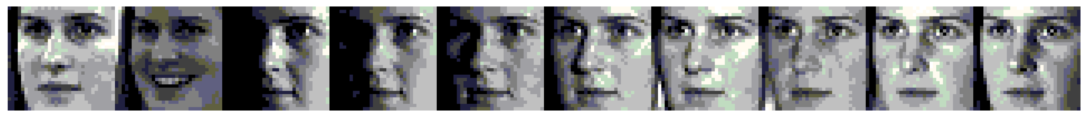
5.1. Experiments on the ORL Face Database

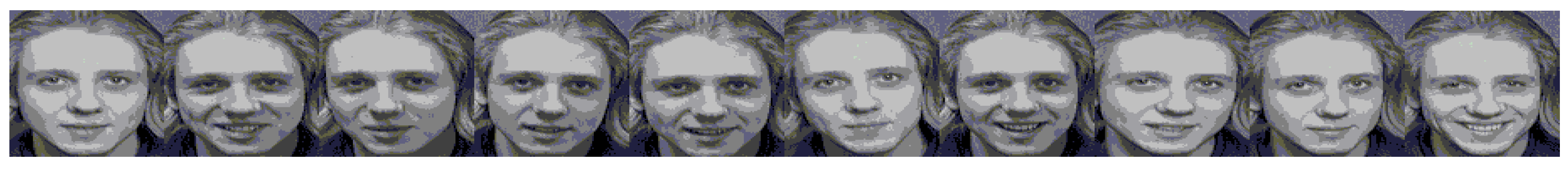
The ORL (Olivetti Research Laboratory) database [39] contains 400 images of 40 persons (10 images per person). To be subjected, the images were taken at different times, varying the light, facial expressions (open or closed eyes, smiling or not smiling), and facial details (glasses or no glasses). The size of each image is 112 × 92 pixels, with 256 gray levels per pixel. In our experiments, the images were normalized and cropped to a resolution of 32 × 32 pixels. Figure 1 shows some sample images of one person from the ORL face database.

The average recognition rates (%) of five different methods used with their correspondent standard deviation and dimension of the best subspace are shown in

Table 1. The average recognition rates of each method on four face databases with the corresponding STDs and dimension of best subspace.

Database	No. of Trains	Eigenface	Fisherface	LPP	NPE	WNPEE
ORL	l = 4	34.02 ± 1.91(41)	66.69 ± 1.21(41)	70.20 ± 0.94(43)	82.05 ± 1.42(37)	84.80 ± 1.22(48)
	l = 5	21.61 ± 0.91(43)	64.62 ± 1.75(47)	74.28 ± 1.46(41)	86.01 ± 1.41(27)	82.56 ± 1.74(37)
	l = 6	18.35 ± 0.73(50)	69.16 ± 1.83(34)	78.76 ± 1.57(24)	86.68 ± 1.42(43)	89.37 ± 1.79(23)
	l = 7	16.18 ± 0.63(50)	71.36 ± 1.92(39)	80.05 ± 1.41(17)	86.05 ± 1.31(22)	86.99 ± 1.78(14)
GT	l = 3	10.24 ± 0.71(50)	30.40 ± 0.72(33)	34.11 ± 0.68(49)	46.28 ± 0.92(24)	47.85 ± 1.94(19)
	l = 5	7.82 ± 0.46(50)	39.51 ± 0.94(37)	49.37 ± 1.53(50)	56.65 ± 1.23(49)	63.84 ± 1.42(22)
	l = 7	7.50 ± 0.35(48)	42.01 ± 0.94(45)	56 ± 1.34(32)	59.59 ± 1.22(39)	69.83 ± 1.48(17)
	l = 9	9.22 ± 0.83(50)	50.40 ± 1.13(41)	59.33 ± 1.33(23)	63.46 ± 1.33(38)	73.26 ± 1.51(20)
CMU PIE	l = 10	70.88 ± 2.43(50)	57.40 ± 2.91(50)	64.05 ± 1.76(50)	62.48 ± 1.84(50)	74.69 ± 1.83(47)
	l = 15	73.24 ± 2.72(48)	77.23 ± 1.22(49)	76.26 ± 2.31(49)	74.54 ± 2.17(47)	84.35 ± 1.91(47)
	l = 20	73.52 ± 2.65(47)	74.50 ± 2.15(48)	82.16 ± 2.14(37)	79.77 ± 2.28(49)	88.13 ± 1.95(31)
	l = 25	76.25 ± 2.61(33)	75.67 ± 2.85(39)	80.17 ± 2.13(33)	79.10 ± 2.25(47)	88.92 ± 1.93(29)
YALE	l = 6	29.57 ± 1.42(47)	43.86 ± 0.98(14)	48.90 ± 0.89(15)	49.22 ± 1.28(24)	55.65 ± 0.90(27)
	l = 7	25.86 ± 1.37(39)	39.86 ± 0.73(24)	48.83 ± 0.91(41)	51.43 ± 0.9(42)	59.33 ± 0.89(25)
	l = 8	23.51 ± 1.27(49)	44.97 ± 1.19(24)	49.95 ± 0.81(35)	55.77 ± 1.14(25)	69.68 ± 1.13(9)
	l = 9	32.53 ± 1.32(47)	47.33 ± 0.90(42)	53.60 ± 0.61(48)	58 ± 1.13(13)	71.80 ± 1.13(20)

. We randomly select $l=4, 5, 6, 7$ images for each individual for training and rest to be used as testing samples. For effective performance, experiments are repeated 10 times for each value of $l$. It can be easily seen from the table that the proposed WNPEE method achieves the best recognition results for value of $l=4, 6, 7$ and NPE has the best recognition when $l=5$. The best average recognition rates for Eigenfaces, Fisherfaces and LPP are, respectively, lower then NPE and WNPEE.

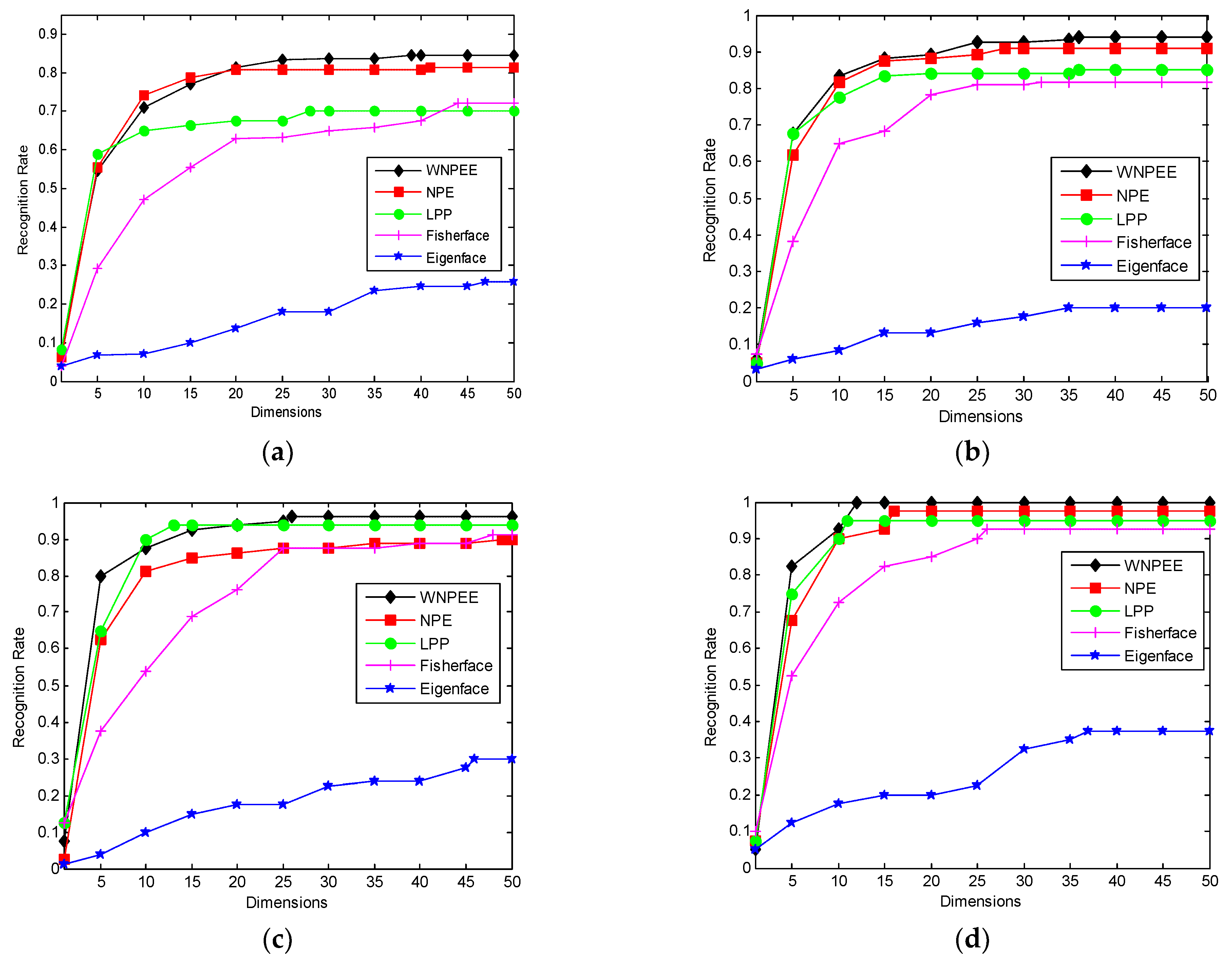
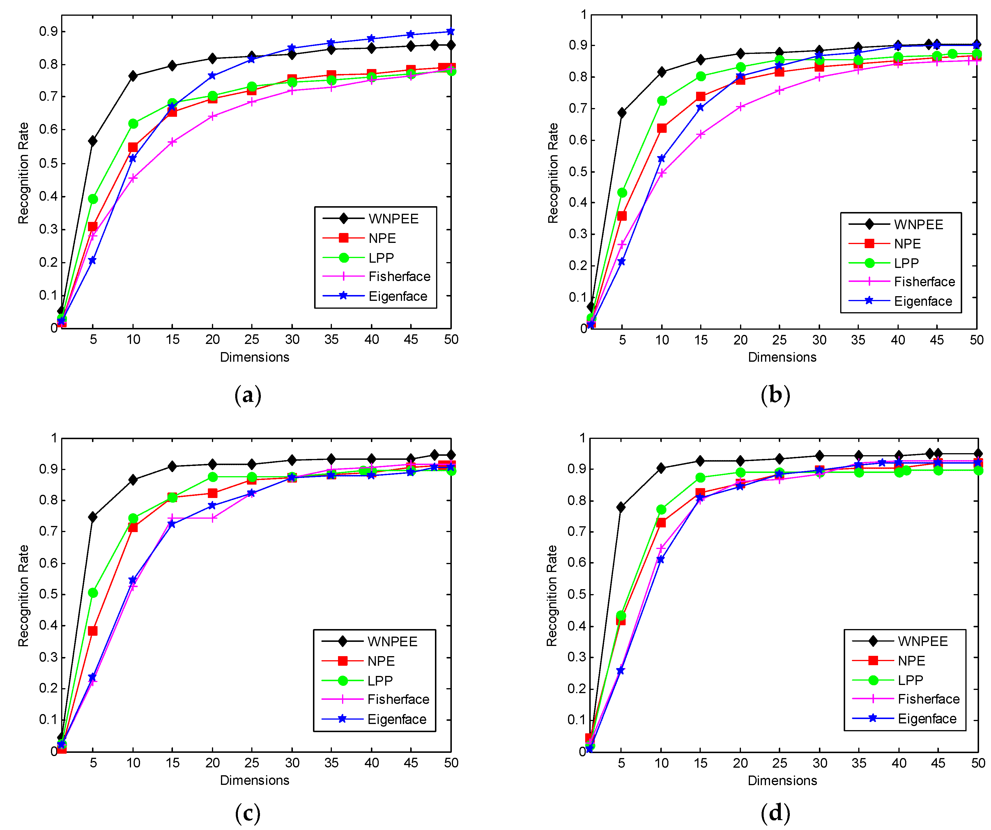
Figure 2 shows the recognition rate versus reduced dimensions of different DR methods used in experiments with our proposed WNPEE algorithm. Figure 2a–d for different values of $l$. From the figures we conclude that Eigenfaces have lowest and proposed WNPEE method have the highest recognition rate. Almost all DR algorithms starts from their lowest value of recognition and achieves the peak value when number of dimensions is 25 and after that almost stable.

We list the computational time (in seconds) of each method for one run with different values of training samples $l$, shown in

Table 2. Computation time on ORL face database under different trains for one run (time in seconds).

No. of Trains	Eigenface	Fisherface	LPP	NPE	WNPEE
l = 3	1.21	1.35	2.16	1.81	2.44
l = 5	2.08	2.87	2.98	2.08	3.16
l = 7	3.07	3.17	3.48	2.27	4.11
l = 9	2.80	2.98	3.74	2.41	4.27
Average	2.29	2.59	3.09	2.14	3.50

. As can be seen from the time results that the time taken by proposed method is slightly more than the other methods and the difference is not much. This is because of one more loop added in our algorithm. However, the performance of the WNPEE is superior to the other algorithms.

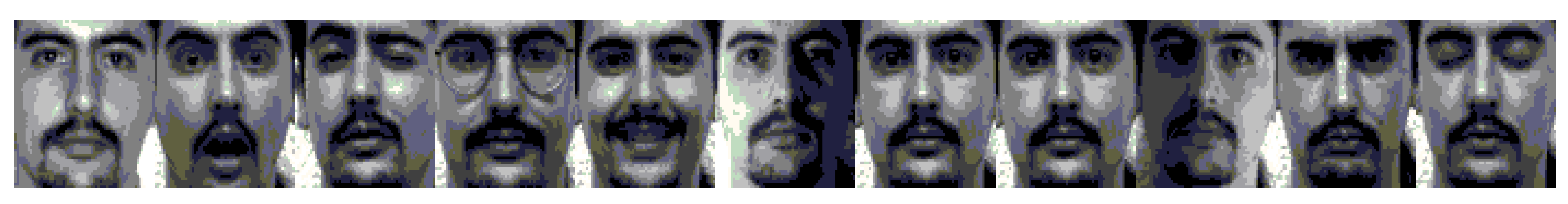
5.2. Experiments on the GT Face Database

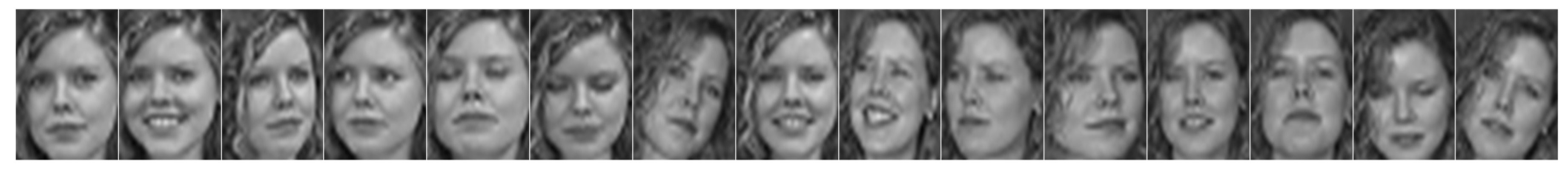
Georgia Tech (GT) face database [40] contains 750 images of 50 people taken in two or three sessions between at the Center for Signal and Image Processing at Georgia Institute of Technology. All people in the database are represented by 15 color JPEG images with cluttered background. These images show frontal and/or tilted faces with different facial expressions, lighting conditions and scale. In our experiments, all the images in the data set were manually cropped to size to 32 × 32 pixels and converted into gray scale images for training and testing. Figure 3 shows some sample images of GT database.

The experimental results in form of average recognition rates (%) of each DR methods with their corresponding standard deviation and best subspace dimension are shown in Table 1. The training sets are chosen randomly with $l=3, 5, 7, 9$ images of each individual and rest to be used as testing samples. For different values of $l$ the experiments are performed for 10 repetitions for satisfactory results. The best results are highlighted in bold face. Results clearly shows that the proposed WNPEE has the best recognition rates among all five comparative DR methods. Additionally, WNPEE achieves its best performance with the increase in value of $l$.

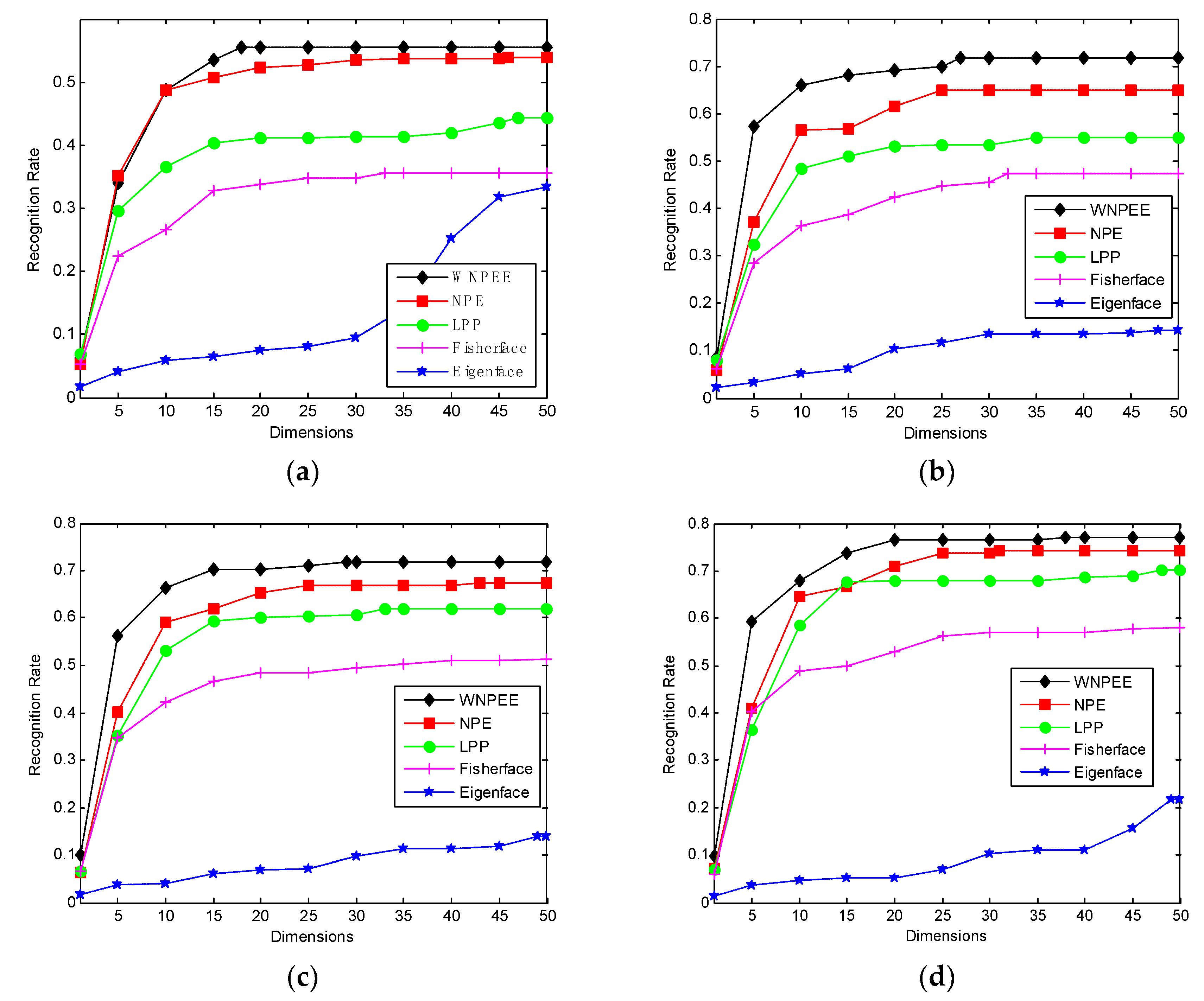
The recognition rate corresponds to reduce dimensions for different DR algorithms are shown in Figure 4a–d for different values of $l$. It is observed from graphs that mostly all comparable methods achieves their peak values of recognition rates in between dimensions 15 to 20 and then becomes stable for higher dimensions. We can also deduce that WNPEE shows the best results whereas NPE overcomes the other three graph-based DR methods.

According to the computational time results shown in

Table 3. Computation time on GT face database under different trains for one run (time in seconds).

No. of Trains	Eigenface	Fisherface	LPP	NPE	WNPEE
l = 3	4.31	4.28	4.31	4.25	4.63
l = 5	5.23	5.12	5.09	5.08	5.78
l = 7	5.72	5.53	5.58	5.54	6.23
l = 9	5.70	5.54	5.62	5.51	7.04
Average	5.24	5.12	5.15	5.09	5.92

, it is detected that the time consumed by WNPEE is different from other methods. On the other hand it shows that the time difference is not so large, it is in some seconds that make our proposed method suitable for many real time applications.

5.3. Experiments on the CMU PIE Face Database

The CMU PIE face database [41] contains 41,368 images of 68 people, each person under 13 different poses, 43 different illumination conditions, and with four different expressions. Images are taken under 15 view points and 19 illumination conditions while displaying a range of facial expressions. All images are moved to gray scale and cropped to 32 × 32 pixels in our experiments. Some sample images are shown in Figure 5.

Table 1 shows the average recognition rates (%) of five DR algorithms with their corresponding standard deviation and best subspace dimension, where the highest rates are in boldface. We choose the first $l=10, 15, 20, 25$ images for the training and rest for the testing samples. Experiments are repeated ten times for best average recognition rates. From the results shown in Table 1 it is found that proposed WNPEE outperform other four comparative DR methods with different training sets. Furthermore, NPE achieves the second best results due to its superiority over other three methods.

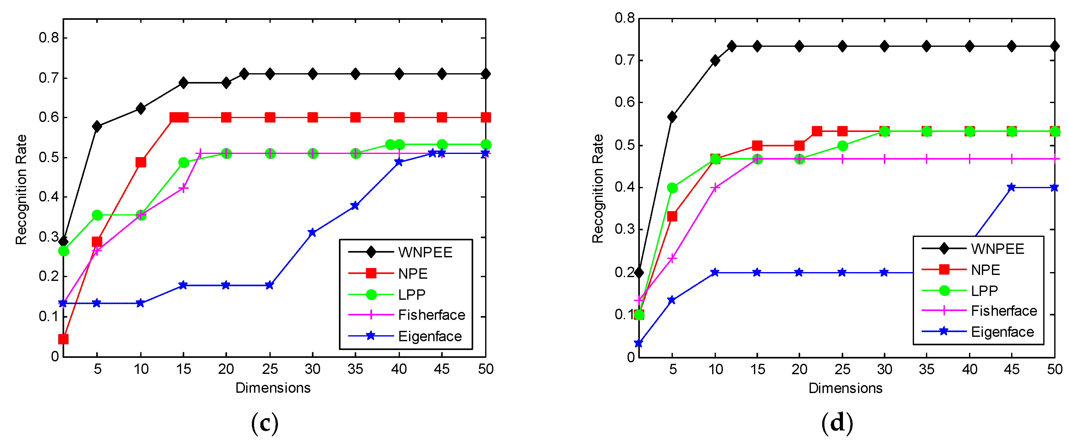
Figure 6a–d illustrates the recognition rate against dimensions for each value of $l$. The graph results demonstrate that our proposed WNPEE outperforms all other comparative DR methods used in experiments. Although when the value of $l=10$, NPE shows more superior recognition but, as the value of $l$ increases, our proposed WNPEE outperforms all methods. It is also noted that with higher values of $l$ overall performance of all DR methods increases.

To evaluate the computation complexity we record the time consumed for all DR techniques for one run which are shown in

Table 4. Computation time on CMU PIE face database under different trains for one run (time in seconds).

No. of Trains	Eigenface	Fisherface	LPP	NPE	WNPEE
l = 3	1.04	2.14	2.57	2.08	2.61
l = 5	1.13	2.23	2.75	2.11	2.79
l = 7	1.12	2.16	2.78	2.13	2.75
l = 9	1.01	2.11	2.95	2.01	3.06
Average	1.07	2.16	2.76	2.08	2.80

. The time is in seconds with different values of trains. Time results reveals that proposed method is almost equal in terms of computations. However, a slight difference in time makes our proposed WNPEE slow, but its performance makes it a competitive algorithm in the field of DR.

5.4. Experiments on the YALE Face Database

The Yale database [42] was used to evaluate the system performance under conditions where the facial expressions and illumination are varied. It contains 165 gray scale images of 15 individuals under various facial expression (normal, happy, sad, sleepy, surprise, and wink), lighting conditions (left-light, center-light, right-light), and facial details (with glasses or without). The original size of the images is 243 × 320 pixels but in our experiments we have normalized each image to 32 × 32 pixels. Some sample images with different face expressions are shown in Figure 7.

In this experiment, we have evaluated the performance of the five methods: Eigenfaces, Fisherfaces, LPP, NPE, and WNPEE. The recognition rates with STDs and dimensions are recorded by taking their mean for 10 runs shown in Table 1. For better implementation of the algorithms different training sets for $l=6, 7, 8, 9$ images of each individual are taken and rest are for testing sets. The result shows the superiority of the WNPEE and also it reveals that with the use of an optimal weighted graph, the performance can be increased for a DR algorithm.

The result graphs are in the form of recognition rate with respect to the dimensions as shown in Figure 8. For different values of $l$ different results are recorded as shown in the figure. Graphs demonstrate two interesting facts, i.e., with a greater amount of training, the greater the accuracy will be, and KNWPE outperforms the other four DR methods in terms of recognition rate. This makes our WNPEE more superior to use in many tasks, including face recognition and pattern analysis.

For any algorithm to be of practical use, it should have a lower computation time. As revealed from

Table 5. Computation time on the YALE face database under different training for one run (time in seconds).

No. of Trains	Eigenface	Fisherface	LPP	NPE	WNPEE
l = 6	0.91	1.9	2.19	2.93	3.03
l = 7	0.93	1.86	2.39	2.89	3.14
l = 8	1.14	1.96	2.94	3.07	3.59
l = 9	1.71	1.87	3.09	4.02	4.65
Average	1.17	1.89	2.65	3.22	3.60

, the overall time for proposed WNPEE is slightly more than the other DR methods with a difference of 0.38 s. The slightly greater time is practically negligible if the performance is far better than the other methods. Thus, we can easily use this proposed WNPEE in practice.

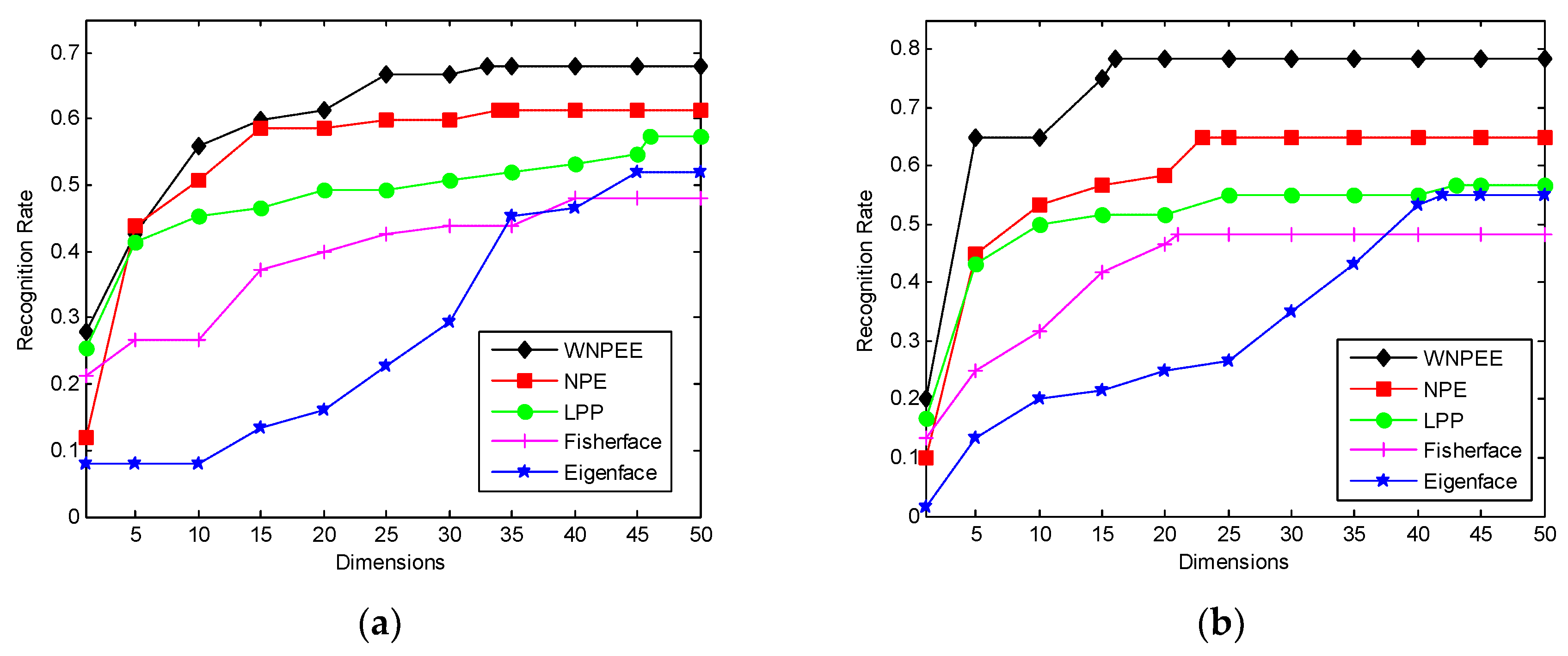
5.5. Analyzing the Sensitivity to Neighborhood Size Parameter

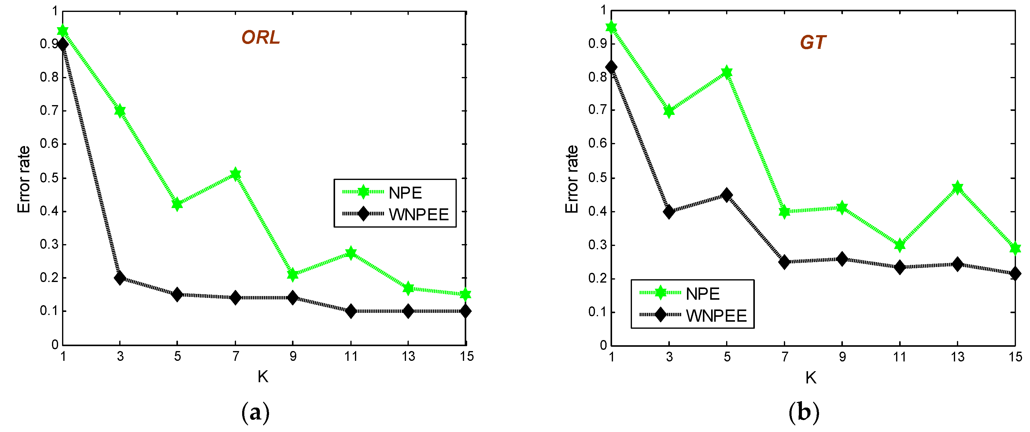
As mentioned before the NPE is among the best graph-based DR methods, but still its performance is very sensitive to the neighborhood size parameter. Thus, to overcome this sensitivity problem in classical NPE we proposed a new WNPEE DR technique. To evaluate the WNPEE sensitivity to the neighborhood size parameter we have conduct experiments on four face databases ORL, GT, CMU PIE, and Yale. The experimental results are observed in form of error rates with varying the parameter of neighborhood size. In these experiments, we vary the value of parameter k from 1 to 15 with a step size of one and plot the corresponding average error rates, as shown in Figure 9. Figure 8a–d are for ORL, GT, CMU PIE, and Yale databases, respectively.

For ORL database, each individual with $l=7$ images are selected randomly for training and rest are used as testing. Figure 8a shows the average error rate versus parameter of neighborhood size on ORL database. From the figure we observe that the error rate for NPE is continuously changing with varying neighborhood size. Firstly it decreases fast when parameter changes from 1 to 3, then suddenly increases up to k = 7, and continue varying with parameter k. On the other hand, the average error rate of our proposed WNPEE shows a sharp down when parameter changes from 1 to 3 and then it is almost stable with contrast of neighborhood size. The above observation clearly shows that proposed WNPEE is very less sensitive to parameter of neighborhood size.

As compared to ORL, Georgia Tech face database is more complex because of increased number of expressions for various pose faces. In our experiment, we choose $l=9$ for everyone to form training and balance were used as testing sets. The average error rates with varying neighborhood size parameter for 10 iterations are presented in Figure 8b. The results show that NPE error rates are different with different value of the neighborhood size parameter. Oppositely, the error rates of WNPEE changes sharply at the start, then up to parameter value 7 it changes little and, further, it become stable. The reason behind this may be the GT database has a very complex bunch of data that needs more time to achieve a stable accuracy as compared to the ORL database.

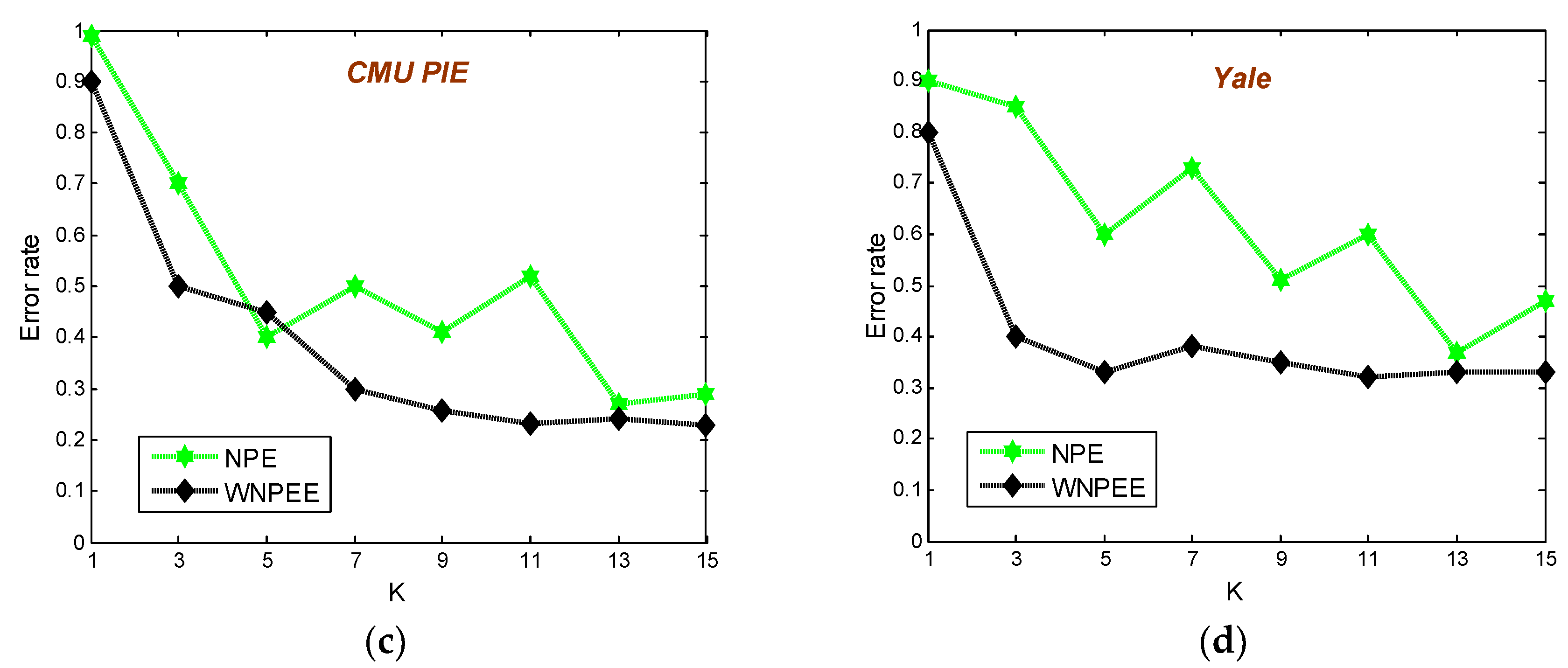
In CMU PIE face database, a random subset of $l=25$ training samples are selected and the rest were taken for the testing set. The average error rates of NPE and WNPEE versus the parameter of neighborhood size for 10 iterations is shown in Figure 8c. Form the plot it is clear that both the error rates for NPE and WNPEE are changing with different values of parameter k, but WNPEE will become stable after k = 7. This shows that WNPE is less sensitive to neighborhood size as compared to NPE.

The Yale database experiment results are shown in Figure 8d. In this experiment, each individual with $l=9$ images are selected as the training set and the rest are taken for the testing set. In the same way, the error rates are used to measure the sensitivity to parameter of neighborhood size. As shown in plot 8d, the performance of the WNPE is less sensitive to the neighborhood parameter than NPE.

Based on the above results on four face databases; we can realize two important facts. First is that NPE accuracy continuously varies with changes in the parameter of neighborhood size. Additionally, the accuracy of proposed WNPEE changes with respect to the neighborhood size parameter, but it becomes relatively stable after the parameter reaches 7 in mostly cases. Another fact is that the proposed WNPEE has attained greater accuracy than NPE in all four experiments. Therefore, an ensemble of adjacent graphs can be utilized to get improved face recognition performance of NPE which is pursued in a joint optimization way. From the above on-going discussions without any obstruction we can conclude that our proposed WNPEE shows a very significant improvement in terms of performance and is less sensitive to the neighborhood size parameter.

5.6. Computation Complexity

The most significant goal for dimension reduction is to help alleviate the problem of data complexities so as to improve the performance of algorithms. In this section, a detailed complexity analysis of the proposed WNPEE algorithm, and the computation cost compared with other approaches on ORL, Georgia Tech, CMU PIE, and Yale datasets are discussed.

The proposed WNPEE algorithm consists of two parts: one is for multiple graph construction and the other is for the iterative solution of the regularization framework. From Algorithm 1, computational convergence of WNPEE subjects to continual update of the weight coefficients ${\alpha }_k$ for multiple adjacent graphs. Suppose a training set $X$ of dimensions $m \mathrm{x} n$, and $k$ number of adjacent graphs for ensemble embedding, then it will take $O\left(k{n}^2\right)$ to compute ${\alpha }_k$. Since our method is an eigenvalue problem, a complexity of $O\left(n^3\right)$ for obtaining the low-dimensional projection vector $a$. Therefore, the total complexity of the proposed WNPEE method is $O\left(t\left(n^3+k{n}^2\right)\right)$, whereis the number of iterations for convergence.

The computation times for obtaining the low-dimensional projections on ORL, Georgia Tech, CMU PIE and Yale datasets are reported in Table 2, Table 3, Table 4 and Table 5. It can be seen that the proposed method is slightly time consuming as compared to the rest of the methods. This is due to the utilization of multiple adjacent graphs in our method. However, the proposed WNPEE obtained superior recognition rates, as shown in Table 1. In conclusion, except for the slightly increased computational time consumption, the proposed WNPEE generally obtains better recognition rates and is less sensitive to neighborhood size k compared to the rest of the DR methods. Thus, there is no constraint to the practical application of the proposed method.

6. Conclusions

In this paper, we proposed a new graph-based DR algorithm, called weighted neighborhood preserving ensemble embedding (WNPEE). The proposed WNPEE method aims at improving the sensitivity of traditional NPE to parameter of neighborhood size, as well as to increase its face recognition performance as compared to other comparative methods. WNPEE significantly enhances the face recognition performance mainly from two key factors. The first improvement resides in the fact that in the WNPEE algorithm constructs an ensemble of adjacent graphs with varying parameters of neighborhood size. With this graph ensemble building, WNPEE can obtain the low-dimensional projections with optimal embedded graph pursuing in a joint optimization way. This helps WNPEE to preserve more local information that best determines the essential manifold structure of high-dimensional data. The second improvement is that WNPEE provides an efficient weighting scheme for eigenspace which makes the projections much less sensitive to the neighborhood size parameter as compared to NPE. Four different DR approaches, Eigenfaces, Fisherfaces, LPP, and NPE, have been compared, to calculate the performance of the proposed WNPEE algorithm. Experimental results on four face databases ORL, GT, CMU PIE, and Yale demonstrate that the proposed WNPEE DR method achieves the highest recognition rates. Additionally, the proposed WNPEE is less sensitive to the neighborhood size parameter when compared to NPE.

Therefore, the proposed WNPEE method can be suitable for advanced driver assistance systems (ADAS) in various tasks, such as object recognition, data classification, obstacle detection, signal processing, text categorization, and various deep learning tasks. In future work we plan to extend ensemble of adjacent graphs framework to other graph embedding techniques.