Article

Three-Phase Three-Level Flying Capacitor PV Generation System with an Embedded Ripple Correlation Control MPPT Algorithm

1
Department of Electrical, Electronic, and Information Engineering, University of Bologna, Viale Risorgimento 2, 40136 Bologna, Italy
2
Department of Electrical and Computer Engineering, Nazarbayev University, 53 Kabanbay Batyr Ave, Astana 010000, Kazakhstan
*
Author to whom correspondence should be addressed.
Electronics 2019, 8(2), 118; https://doi.org/10.3390/electronics8020118
Submission received: 19 December 2018 / Revised: 21 January 2019 / Accepted: 21 January 2019 / Published: 22 January 2019
(This article belongs to the Special Issue Renewable Electric Energy Systems)

Abstract

:
This paper presents the implementation of a maximum power point tracking (MPPT) algorithm in a multilevel three-phase photovoltaic (PV) system using the ripple correlation control (RCC) method. Basically, RCC adopts the inherent oscillations of PV current and voltage as perturbation, and it has been predominantly used for single-phase configurations, where the oscillations correspond to the 2nd order harmonics. The implementation of an RCC-MPPT algorithm in a three-phase system has not been presented yet in the literature. In this paper, the considered three-phase three-level converter is a three-level flying capacitor (FC) inverter. The proffered RCC method uses the 3rd harmonic components of PV current and voltage for the estimation of the voltage derivative of the power dPpv/dVpv (or current, dIpv/dVpv), compelling the PV array to operate at or very close to the maximum power point. The analysis and calculation of the low-frequency PV current and voltage ripple harmonic components in the three-phase flying capacitor inverter is presented first, with reference to centered carrier-based three-level PWM. The whole grid-connected PV generation scheme has been implemented by MATLAB/Simulink, and detailed numerical simulations verified the effectiveness of the control method in both steady-state and dynamic conditions, emulating different sun irradiance transients.

1. Introduction

To fulfill the constantly increasing worldwide energy demand, renewable energy sources such as photovoltaic (PV), wind, geothermal, and biomass, are being explored. Currently, PV energy is becoming one of the most widely used renewable energy sources, due to its indubitable known advantages and the decreasing installation costs.
In order to improve the PV conversion efficiency, maximum power point tracking (MPPT) algorithms are widely adopted in both grid-connected and stand-alone PV systems. Among the different methods known in the literature, the most popular and effective are perturb and observe (P&O) [1] and incremental conductance [2]. Typical problems for these methods are the identification of a suitable perturbation step size, and the limited maximum power point (MPP) tracking dynamic capability during sudden variations in solar irradiance. In this class of P&O algorithms, either fixed or variable step size are adopted to improve the settling time in transient conditions and the MPP resolution in the steady-state operating points [3].
Similar to P&O techniques, the extremum seeking (ES) algorithm employs “ad hoc” perturba-tions [4]. A multi-variable extremum seeking algorithm based on a single control loop for cascaded dc/dc photovoltaic micro-converters has been proposed in [5]. A Newton-based ES algorithm has been adopted to improve the dynamic performances of gradient-based ES in [6]. All aforementioned algorithms implemented the ES control by injecting an external perturbation signal into the duty cycle. On the contrary, ripple correlation control (RCC) algorithms exploit the inherent PV voltage and current oscillations to track the MPP. In particular, for single-phase PV systems the 2nd harmonics are exploited [4,7,8,9,10,11,12,13]. The RCC algorithm has good dynamic performance comparing with the P&O algorithms and it does not require additional perturbations in tracking the MPP. A comprehensive analysis and comparison between RCC and ES methods has been carried out in reference [9] in case MPPT algorithms for PV systems.
The basic RCC-MPPT method has been investigated in references [9,12,14] where two low-pass filters and two high-pass filters are used for ripple extraction and implementation. In reference [10], a modified RCC method has been proposed by using the moving average concept instead of high/low-pass filtering to improve the dynamic response, without the need to tune the time constant of the low/high pass filters. Moreover, the scheme has been simplified by using only the sign of the product of power and voltage ripple to drive the PV operating point toward the MPP. In reference [13], a hybrid RCC-MPPT algorithm has been proposed to improve stability during sudden solar irradiance transients. In case of three-phase two-level (2L) inverters, the RCC algorithm cannot be applied due to the inexistence of inherent (natural) low-order harmonic oscillations on the PV side of the inverter. In this case, the ES algorithm can be successfully applied by means of additional perturbations, as reported in reference [15].
In recent years, multilevel inverters have become more attractive for single- and three-phase systems thanks to their advantages over the conventional inverters [7,15,16,17,18,19]. They offer improved output waveforms, lower total harmonic distortion (THD) and smaller grid filter size [20,21,22]. The most common multilevel converter configurations, presented in literature, are the cascaded H-bridge (CHB), neutral-point-clamped (NPC) and flying capacitor (FC). These types of converters are also adopted in PV applications due to the aforementioned advantages. Multilevel flying capacitor inverters have some specific distinct advantages over the other two topologies such as: no need for many isolated dc sources when compared to CHB inverters, no need for clamping diodes in contrast to NPC inverters, but still preserving the ability to self-balance the capacitor voltages.
With reference to the FC inverter, several analyses have been presented in the literature. A mathematical model for the dynamic behavior of a simple FC inverter using a sampled-data modeling approach has been derived in reference [23], with useful information on the power circuit characteristics and its natural balancing property. In reference [24], a modified pulse with modulation (PWM) strategy is introduced to improve the balancing rate of capacitor voltages, mainly for small output voltages, by optimizing the use of redundancy of switching states. A new PWM scheme has been proposed and analyzed in reference [25], which results in better balancing properties than the normal phase-shifted (PS) PWM. In particular, a five-level configuration has been considered and a modified PS-PWM scheme has been studied, solving the slow-balancing problems of the normal PS-PWM method for odd-level of FC converters.
In general, adopting a multilevel inverter introduces different low-order voltage and current harmonics on the dc-link side compared to the case of a single-phase H-bridge inverter where only the 2nd order harmonics are present. The application of the RCC algorithm in case of a single-phase inverter with level doubling network (LDN) has been introduced and examined in reference [10]. Due to the multiple harmonics, the basic implementation of the RCC-MPPT scheme becomes deficient, leading to a misestimating of the voltage derivative of the power (dPpv/dVpv). For this reason, a modified RCC scheme extracting the amplitude of a definite harmonic form PV voltage and current (dc-link) waveforms has been proposed. In order to maximize the resolution, the proposed solution makes reference to the highest amplitude harmonic, leading to a more effective estimation of dPpv/dVpv.
Though numerous RCC-MPPT algorithms for single-phase grid-connected PV systems have been developed, no analysis of RCC-MPPT in case of three-phase multilevel inverters has been reported. This paper presents an RCC-MPPT algorithm for a grid-connected three-phase three-level FC inverter (Figure 1) with reference to centered level-shifted (LS) carrier-based PWM modulation. Moreover, a complete analysis of PV voltage and PV current harmonic components is accomplished, being the foundation of the ripple correlation control. In this case, dc-link voltage and current harmonics are introduced by the instantaneous power oscillations between the three flying capacitors and the dc bus, consisting mainly of 3rd harmonic components. These voltage and current harmonics are exploited as embedded perturbations to determine the MPP of the PV array. The considered grid-connected three-phase PV generation system is presented in the block diagram of Figure 1.

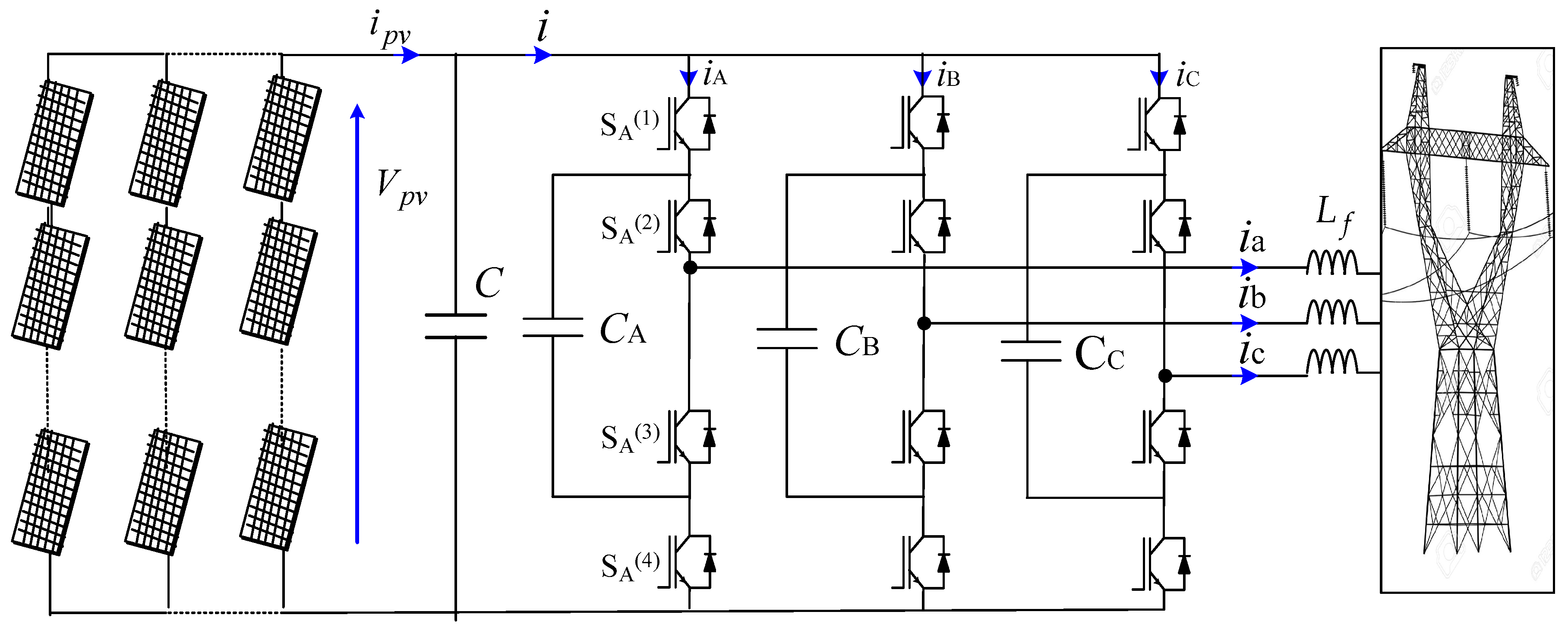
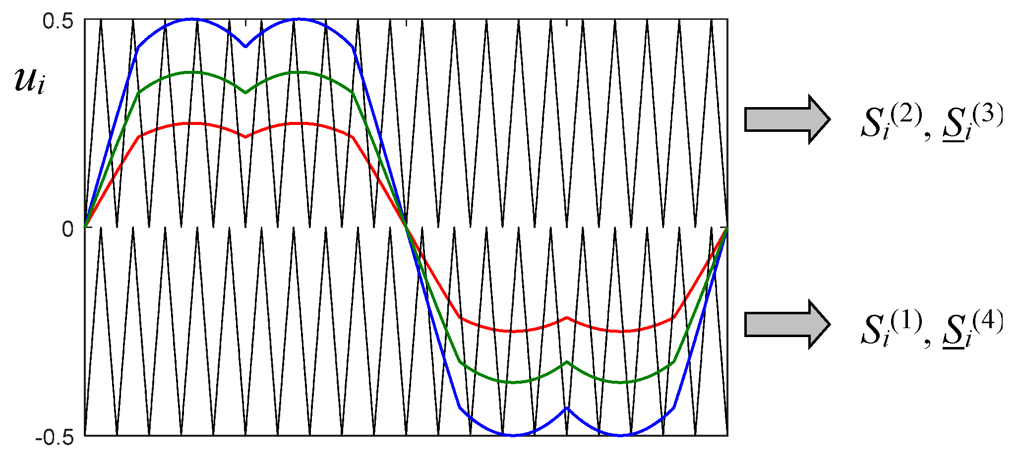
2. Modulation Principle for the Three-Level FC Inverter

With reference to linear and balanced sinusoidal modulation, the modulating signals (uA, uB, and uC) correspond to the inverter output voltages (vA, vB, and vC) normalized by Vpv and averaged over the switching period (Tsw = 1/fsw):
{ u A = m sin ( ϑ ) + C m = u A * + C m u B = m sin ( ϑ 2 π 3 ) + C m = u B * + C m u C = m sin ( ϑ 4 π 3 ) + C m = u C * + C m ,
where ϑ = ωt is the phase angle, ω is the fundamental (angular) frequency, m is the modulation index, u i * are the reference (normalized) output voltages (i = A, B or C), and Cm is the common-mode signal to maximize the linear modulation range.
The voltages across the flying capacitors CA, CB and CC are spontaneously regulated to the half of the DC-link voltage if a proper modulation technique with self-balancing capability is adopted [19]. Introducing for the upper switch of each phase i (i = A, B, C) the switching function S ¯ i ( 1 ) (averaging is denoted in the following by overline) results in:
S ¯ i ( 1 ) = u i | u i | + 1 .
With reference to phase A, considering Equations (1) and (2), it becomes:
S ¯ A ( 1 ) = m sin ( ϑ ) + C m | m sin ( ϑ ) + C m | + 1 .
The switching functions for the other phases B and C are readily obtained by exploiting the modulation symmetry among the three phases, according to Equation (1).
In order to improve the so-called sinusoidal PWM (SPWM), in which there is no common-mode signal injection, Cm = 0, one of the most popular ways to maximize the modulation index is the so called “centered” PWM (CPWM), consisting of the injection of a common-mode signal able to center the modulating signals:
C m = 1 2 [ max ( u A * , u B * , u C * ) + min ( u A * , u B * , u C * ) ] .
In case of sinusoidal reference voltages, Equation (1), Cm can be rewritten as:
C m = 1 2 m { sin ϑ , π 6 ϑ π 6 , 5 π 6 ϑ 7 π 6 sin ( ϑ + 2 π 3 ) , π 6 ϑ π 2 , 7 π 6 ϑ 3 π 2 sin ( ϑ 2 π 3 ) , π 2 ϑ 5 π 6 , 3 π 2 ϑ 11 π 6 .
Figure 2 shows an example of the considered carrier-based CPWM strategy for three different modulation indices.

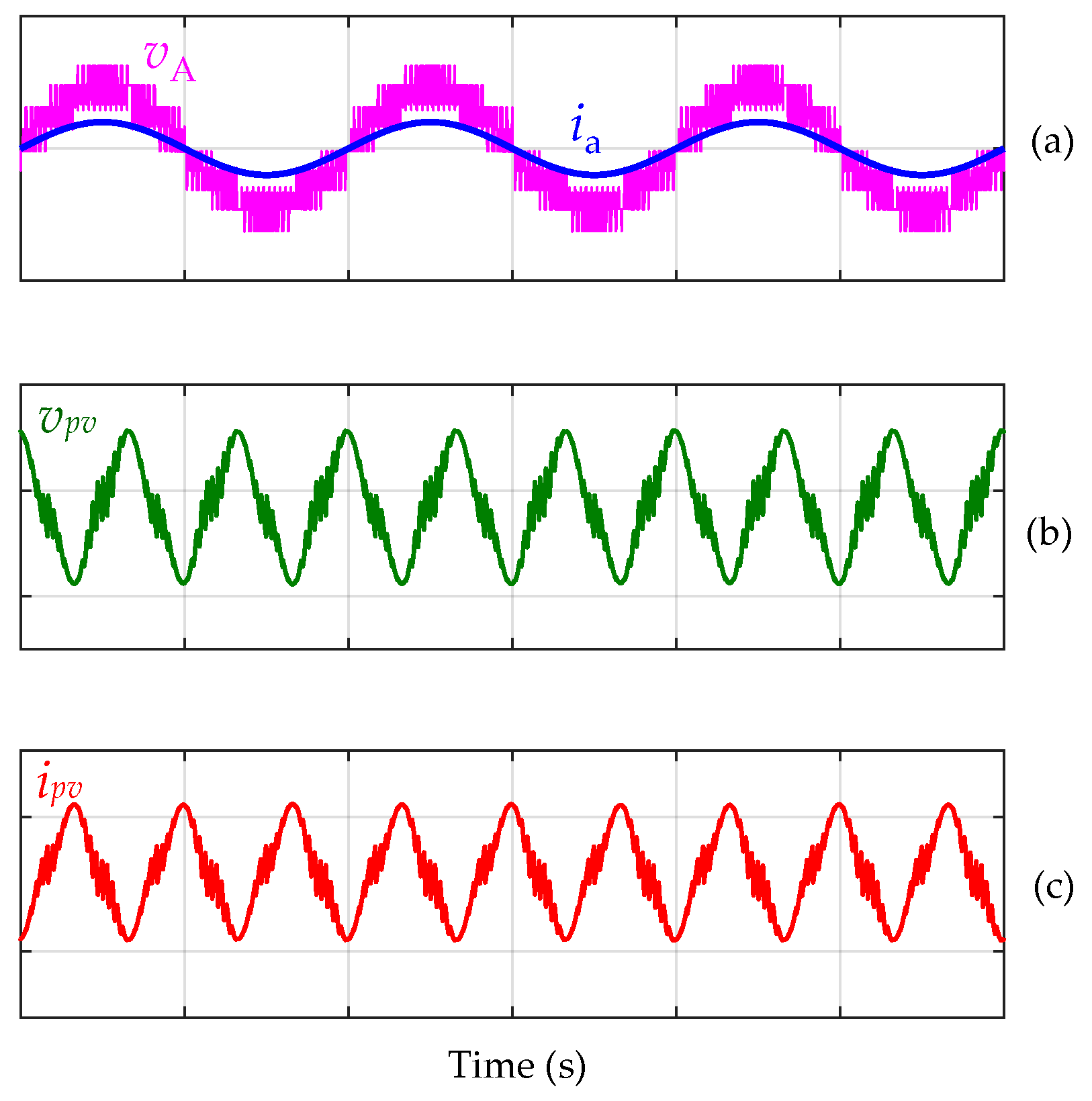
3. Evaluation of PV Current and Voltage Harmonics

In the studied single-stage PV generation system (Figure 1), the PV array is directly connected to the dc-link bus of the three-phase FC inverter. In this way, PV voltage harmonics correspond to the inverter dc-link voltage harmonics, whereas PV current harmonics can be calculated on the basis of the inverter dc-link current harmonics by the following procedure.

3.1. Inverter Input Current Harmonics

The instantaneous inverter input current i(t) consists of the averaged component over the switching period i ¯ , and the instantaneous switching ripple component Δ i . Similarly, the current averaged over the switching period consists of its averaged component over the fundamental period Idc (dc component) and the alternating low-frequency harmonic component i ˜ . These compositions are summarized as:
i ( t ) = i ¯ + Δ i = I d c + i ˜ + Δ i .
Neglecting the switching ripple, the output currents can be considered a sinusoidal balanced system with the amplitude Iac and the general output phase angle φ comparing to grid voltages:
{ i a = I a c sin ( ϑ φ ) i b = I a c sin ( ϑ 2 π 3 φ ) i c = I a c sin ( ϑ 4 π 3 φ ) .
For each inverter leg, the averaged input current (over the switching period) can be determined by multiplying the switching function of upper switch by the corresponding output current. With reference to leg A, it leads to:
i ¯ A = S ¯ A ( 1 ) i a .
By introducing Equations (3) and (7) in Equation (8), the averaged current of the leg A becomes:
i ¯ A = I a c sin ( ϑ φ ) [ m sin ( ϑ ) + C m | m sin ( ϑ ) + C m | + 1 ] .
The resulting averaged total input current i ¯ is the sum of the three leg currents:
i ¯ = S ¯ A ( 1 ) i a + S ¯ B ( 1 ) i b + S ¯ C ( 1 ) i c .
In the following, the analysis is restricted to the phase angle span 2π/3 since the inverter input current has a periodicity of T/3. In particular, with reference to the phase angle range 2π/3 ≤ ϑ ≤ 4π/3, the inverter input current can be expressed in the following two sub-ranges π/3:
i ¯ = { ( S C ( 1 ) 1 ) i c , 2 π 3 ϑ π S A ( 1 ) i a + i b + S C ( 1 ) i c , π ϑ 4 π 3 .
Introducing Equations (1), (2), and (7) in Equation (11) leads to:
i ¯ = m I a c 2 { 3 [ cos ( 2 ϑ 3 π 2 φ ) + cos ( π 6 + φ ) ] ,   2 π 3 ϑ 5 π 6 3 [ cos ( 2 ϑ + π 6 φ ) + cos ( π 6 φ ) ] , 5 π 6 ϑ π 3 [ cos ( 2 ϑ 7 π 6 φ ) + 1 2 cos ( π 2 φ ) + 3 3 2 cos ( φ ) ] ,   π ϑ 7 π 6 [ 3 cos ( 2 ϑ 3 π 2 φ ) cos ( π 3 φ ) + 5 cos ( φ ) ] , 7 π 6 ϑ 4 π 3 .
By examining Equation (12), the average and the low-frequency input current components can be determined in case of centered PWM as:
I d c = 3 2 m I a c cos ( φ ) ,
i ˜ = m I a c 2 { 3 [ cos ( 2 ϑ 3 π 2 φ ) + cos ( π 6 + φ ) 3 cos ( φ ) ] ,   2 π 3 ϑ 5 π 6 3 [ cos ( 2 ϑ + π 6 φ ) + cos ( π 6 φ ) 3 cos ( φ ) ] , 5 π 6 ϑ π 3 [ cos ( 2 ϑ 7 π 6 φ ) + 1 2 cos ( π 2 φ ) + 3 2 cos ( φ ) ] ,   π ϑ 7 π 6 [ 3 cos ( 2 ϑ 3 π 2 φ ) cos ( π 3 φ ) + 2 cos ( φ ) ] , 7 π 6 ϑ 4 π 3 .
Although the above developments are carried out for centered PWM, the input inverter current analysis can be similarly extended to other PWM techniques. As an example, the simpler case of sinusoidal PWM has been presented in reference [21].
In order to prove the validity of Equations (12)–(14), some simulation tests concerning the input inverter currents, with specific reference to unity power factor (φ = 0°) and unity sinusoidal output currents (Iac = 1A), are presented in Figure 3.
In particular, top traces in Figure 3 show the simulation results comparing the instantaneous input current of leg A iA (blue trace) with its averaged value over the switching period i ¯ A (red trace), and the corresponding low-frequency current component calculated by replacing Equation (5) in Equation (9) (green trace). Two cases of modulation index m = 0.577/2 (Figure 3, left) and m = 0.577 (Figure 3, right) are considered.
The bottom traces in Figure 3 show the total instantaneous inverter input current i(t) (blue trace) and its averaged value over the switching period i ¯ (red trace). The averaged current component (green trace) is determined analytically in case of centered PWM by Equation (12). Figure 3 shows a perfect matching between theoretical and simulated results. The slight delay (Tsw/2) between numerically averaged values and the corresponding theoretical averaged values is due to the numerical averaging itself.

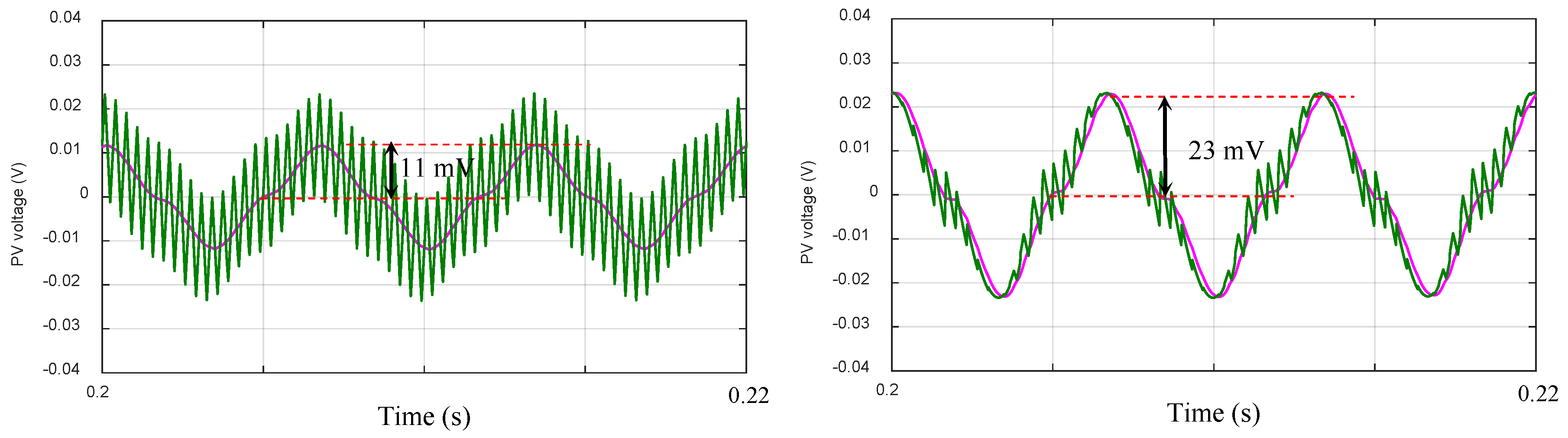
3.2. PV Voltage Harmonics

Similarly to the input dc-link current, dc-link voltage components can also be pointed out. The instantaneous dc-link voltage vpv, corresponding to the PV voltage, consists of its averaged value over the switching period v ¯ p v and the instantaneous switching ripple Δvpv. Also, the averaged component over the fundamental period Vpv (dc component) and the low-frequency harmonic component v ˜ p v can be introduced, leading to:
v p v = v ¯ p v + Δ v p v = V p v + v ˜ p v + Δ v p v V p v + v ˜ p v .
The switching ripple component Δvpv is practically insignificant for switching frequencies starting from few kHz, being completely smoothed by the dc-link capacitor. For this reason, it is assumed here to be Δvpv ≈ 0. The alternating low-frequency voltage component can be evaluated based on the low-frequency input current component taking i ˜ into account the whole dc-link impedance, given by the parallel of the capacitor reactance and the equivalent resistance of the PV array at maximum power point (RpvVmpp/Impp).
Taking into consideration the expected parameters for PV arrays and dc-link capacitors, the assumption Rpv >> 1/(kωC) is usually true, with k being the harmonic order. In this case, the whole alternating input current component is circulating through the dc-link capacitor, and the alternating dc-link (PV) voltage component can be calculated by integrating Equation (14). The resulting four contributions can be adopted in order to calculate the amplitude (peak value) of the alternating low-frequency voltage component:
{ Δ V ˜ p v , 1 = m I a c ω C [ π 8 3 sin φ + 2 3 π 8 cos φ ] Δ V ˜ p v , 2 = m I a c ω C [ π 8 3 sin φ + 2 3 π 8 cos φ ] Δ V ˜ p v , 3 = Δ V ˜ 1 Δ V ˜ p v , 4 = Δ V ˜ 2 .
As most of the grid-connected PV systems operate under unity power factor conditions, the case φ = 0° is considered in the following developments. In this case, the peak of the alternating low-frequency voltage ripple is calculated taking into account either the first or the second contribution, leading to:
V ˜ p v = m I a c ω C 2 3 π 8 0.04 I a c ω C m .
Equation (17) presents the peak value of the alternating voltage ripple in case of CPWM with reference to φ = 0. However, the peak value of the same quantity has been determined in case of SPWM in reference [21] as:
V ˜ p v 0.167 I a c ω C m .
Comparing Equations (17) and (18), it should be noted that practically the peak value of the alternating low-frequency voltage ripple in case of CPWM is almost four times less than the voltage ripple in the case of SPWM.
As an example, the instantaneous PV voltage is shown in Figure 4 (green trace) together with its averaged value over the switching period (pink trace) in case of IacC = 1 for two cases of modulation indices m = 0.577/2 and m = 0.577. A small delay between averaged and instantaneous values (Tsw/2) can be noticed, due to the averaging itself. The peak value of the alternating PV voltage component corresponds to the result obtained by Equation (17). In particular, v ˜ p v is equal to 0.011 V and 0.023 V for m = 0.577/2 and m = 0.577, respectively.
As expected, there is a very good matching between simulation and analytical results.

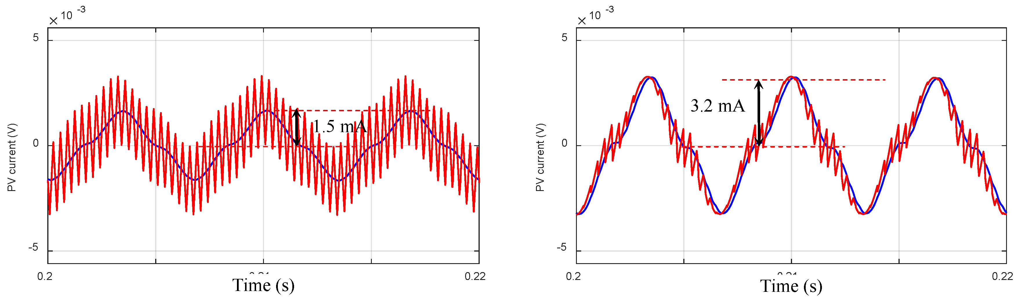
3.3. PV Current Harmonics

With regard to the PV voltage vpv (Equation 15) and neglecting the switching frequency component, the instantaneous PV current ipv can be written as:
i p v = I p v + i ˜ p v ,
being Ipv the average over the fundamental period (Ipv = Idc, due to the dc-link capacitor) and i ˜ p v the alternating low-frequency harmonic component, calculated as:
i ˜ p v = v ˜ p v / R p v .
The amplitude of the alternating low-frequency PV current ripple is calculated based on Equations (17) and (20) as:
I ˜ p v = 2 3 π 8 I a c R p v ω C m 0.04 I a c R p v ω C m .
As an example, Figure 5 shows the instantaneous PV current (red trace) together with its averaged value over the switching period (blue trace) in case of IacC = 1 and for two cases of modulation index, considering a PV series equivalent resistance Rpv = 7.13 Ω, representing the scale factor with Figure 4.

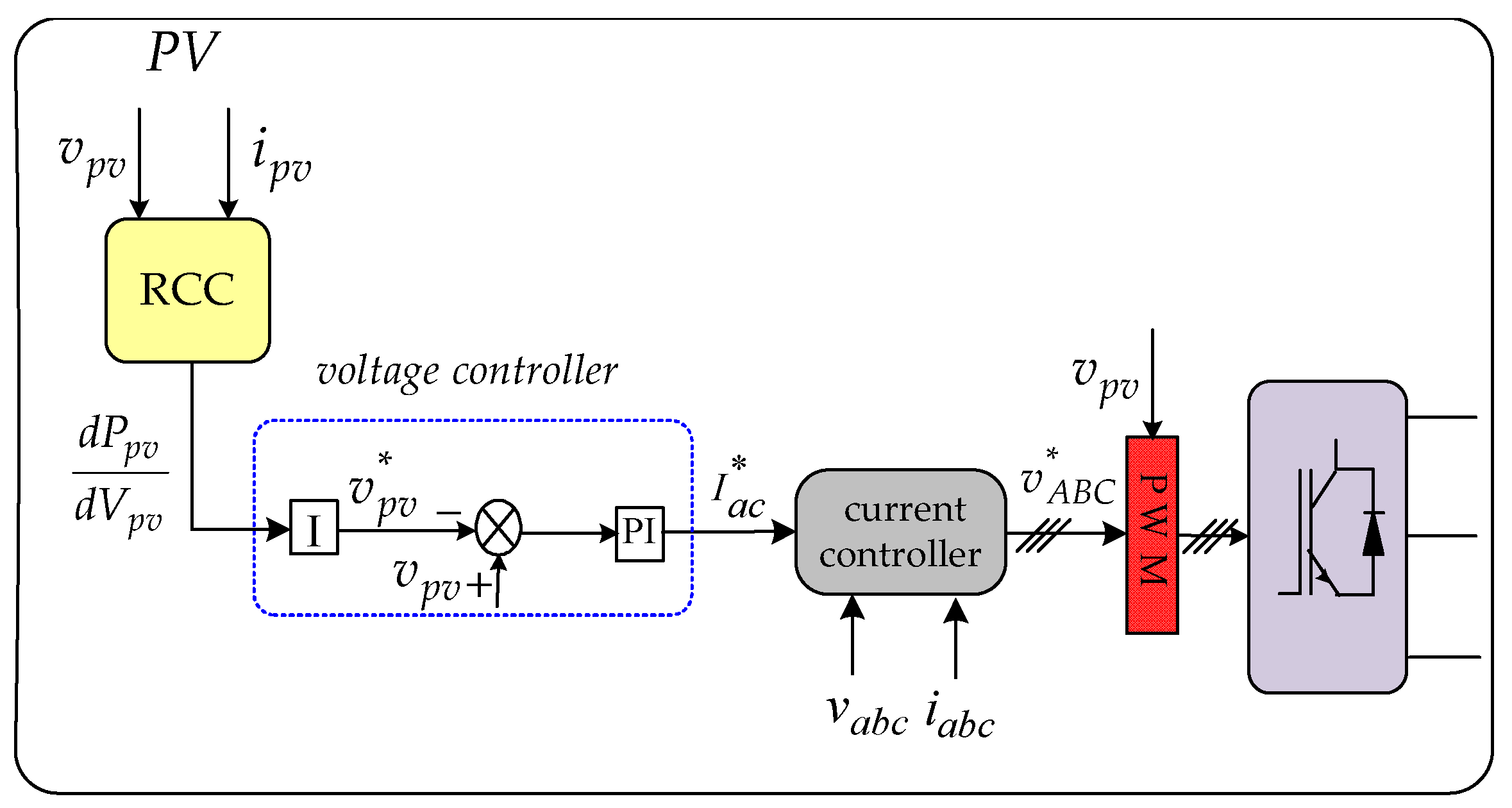
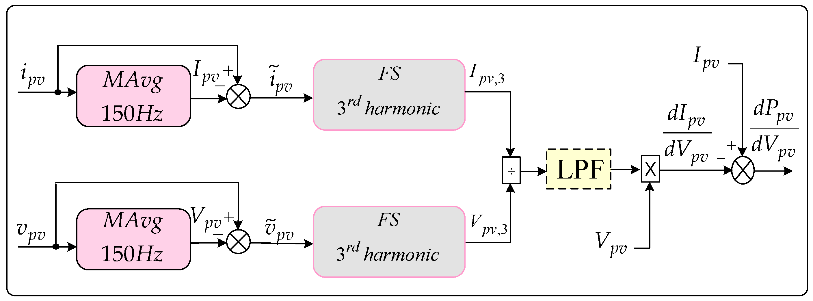
4. Proposed RCC-MPPT Algorithm

Figure 6 presents the block diagram of the adopted control scheme, including MPPT and dc-link (PV) voltage regulation. In particular, the proposed RCC algorithm estimates the voltage derivative of the power, dPpv/dVpv, used to drive the working point to the maximum power point. Integrating dPpv/dVpv, the reference dc-link voltage vpv* is simply obtained and a proportional-integral (PI) voltage regulator can be used to determine the reference grid current amplitude Iac*. In order to inject a sinusoidal current into the grid with unity power factor, a traditional dq current controller has been used.
An example of PV voltage and current ripple in case of a three-phase FC inverter configuration is given in the following. Figure 7 shows the results considering the PV conversion scheme for a given operating point. As expected, the inverter voltage has nine levels for a higher modulation index. Also, it is noticeably clear that PV voltage and current contain a huge 3rd harmonic component (150 Hz) and are in phase opposition.
In case of three-phase PV systems, with the inverter being directly connected to the PV array, the FC inherent 3rd (and odd multiple) order harmonic appears in PV current and PV voltage (as shown in Figure 7). As is known, ripple correlation control algorithm is able to exploit the amplitude of these oscillations to provide information about the operating point of the PV array. Considering the working point Q, the voltage derivative of the PV power dPpv/dVpv can be s written as:
d P p v d V p v | Q = I p v + d I p v d V p v | Q V p v ,
where dIpv/dVpv is defining the voltage derivative of the current as:
i ˜ p v = d I p v d V p v | Q v ˜ p v .
A conventional RCC-MPPT algorithm is implemented by multiplying the voltage oscillation by the current oscillation, and integrating over the harmonic period [10]. As an alternative implementation, the estimation of dIpv/dVpv (and then dPpv/dVpv) can be carried out by considering a specific harmonic order, which is the 3rd in the case of the FC inverter. Equation (23) can be then rewritten as:
i ˜ p v , 3 = d I p v d V p v | Q v ˜ p v , 3 .
By following the approach of the conventional RCC-MPPT implemented in [10], the estimation of the voltage derivative of the current dIpv/dVpv can be calculated, considering the third harmonic component as:
d I p v d V p v | Q 3 = t T t i ˜ p v , 3 v ˜ p v , 3 d t t T t v ˜ p v , 3 2 d t = I p v , 3 V p v , 3 V p v , 3 2 = I p v , 3 V p v , 3 .
It should be noted that dIpv/dVpv derived by Equation (25) is calculated by integrating the product of the PV voltage and current over the fundamental period T, as defined by Fourier series (FS) to calculate the 3rd harmonic. The block diagram of Figure 8 shows a possible implementation of Equation (25), with the estimation of dPpv/dVpv considering only the 3rd harmonic component.

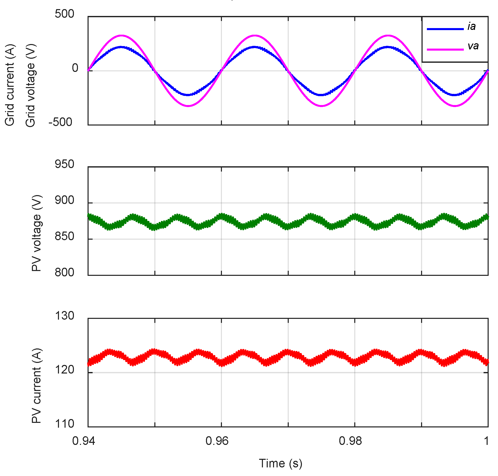
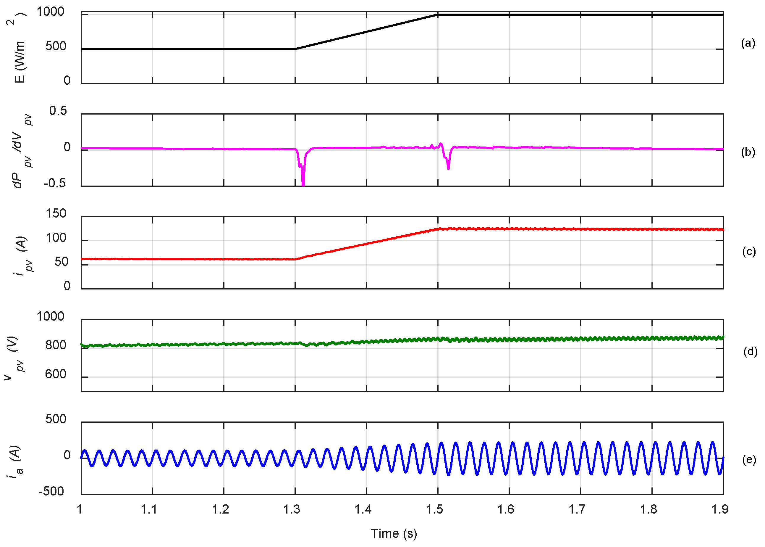
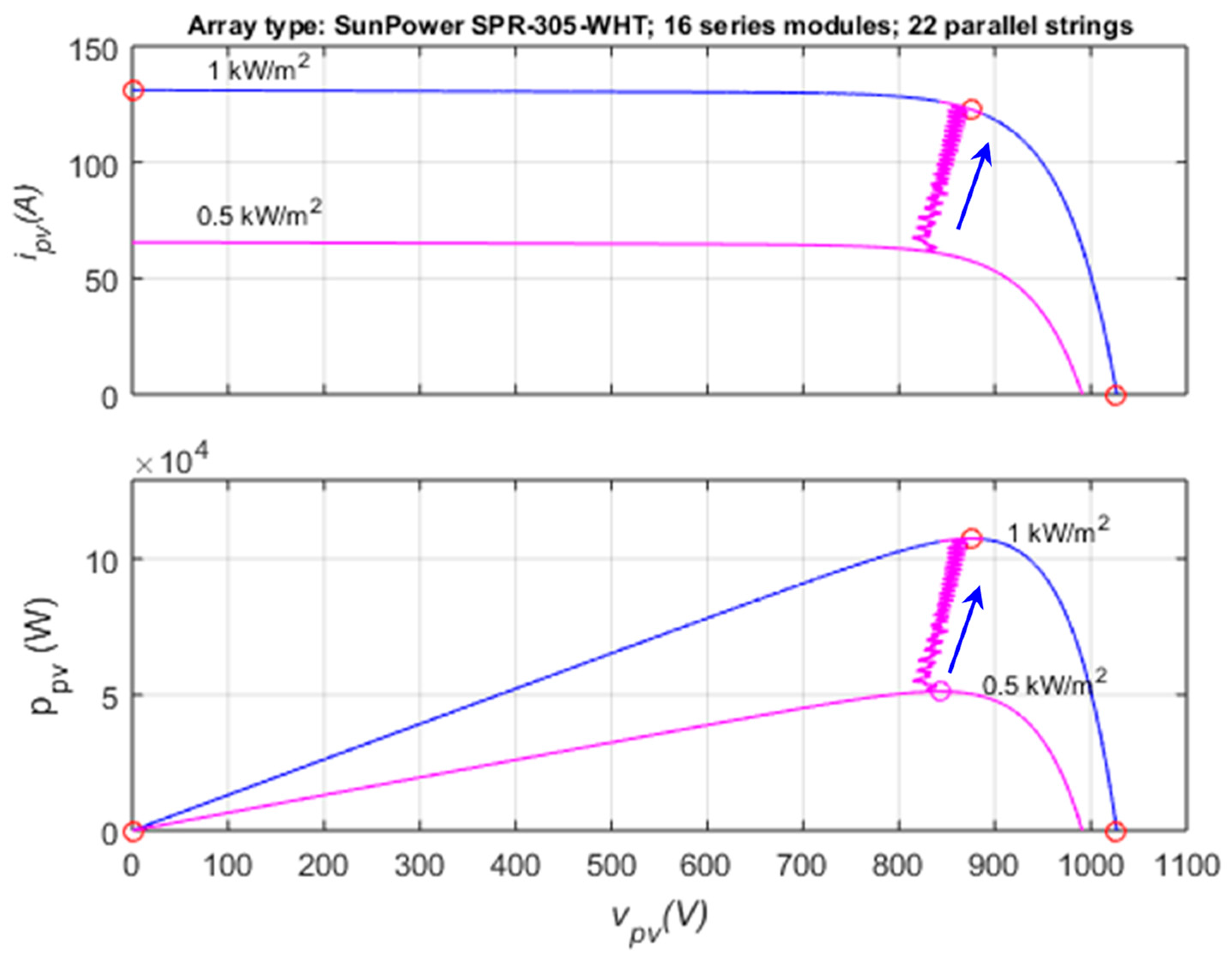
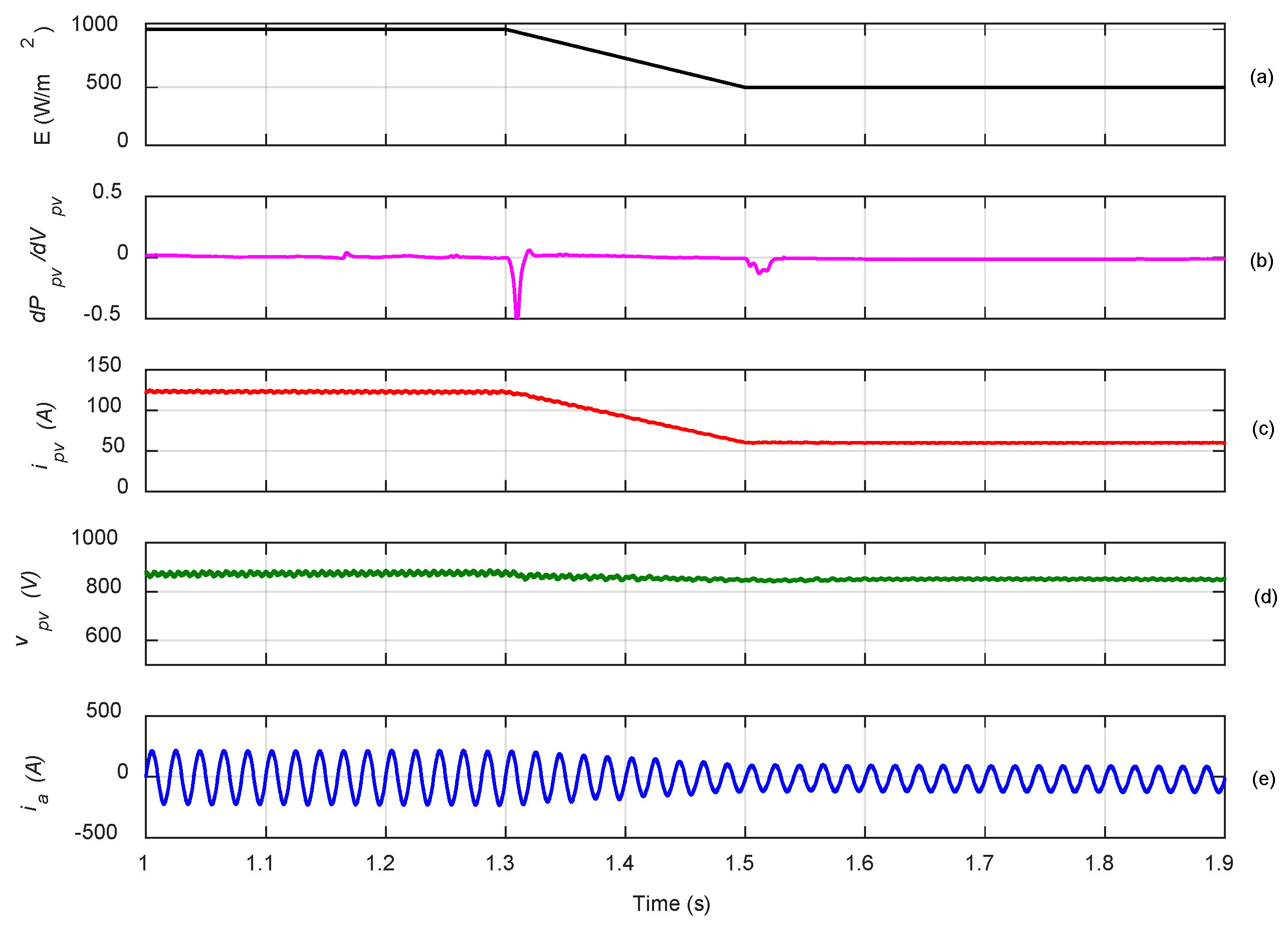
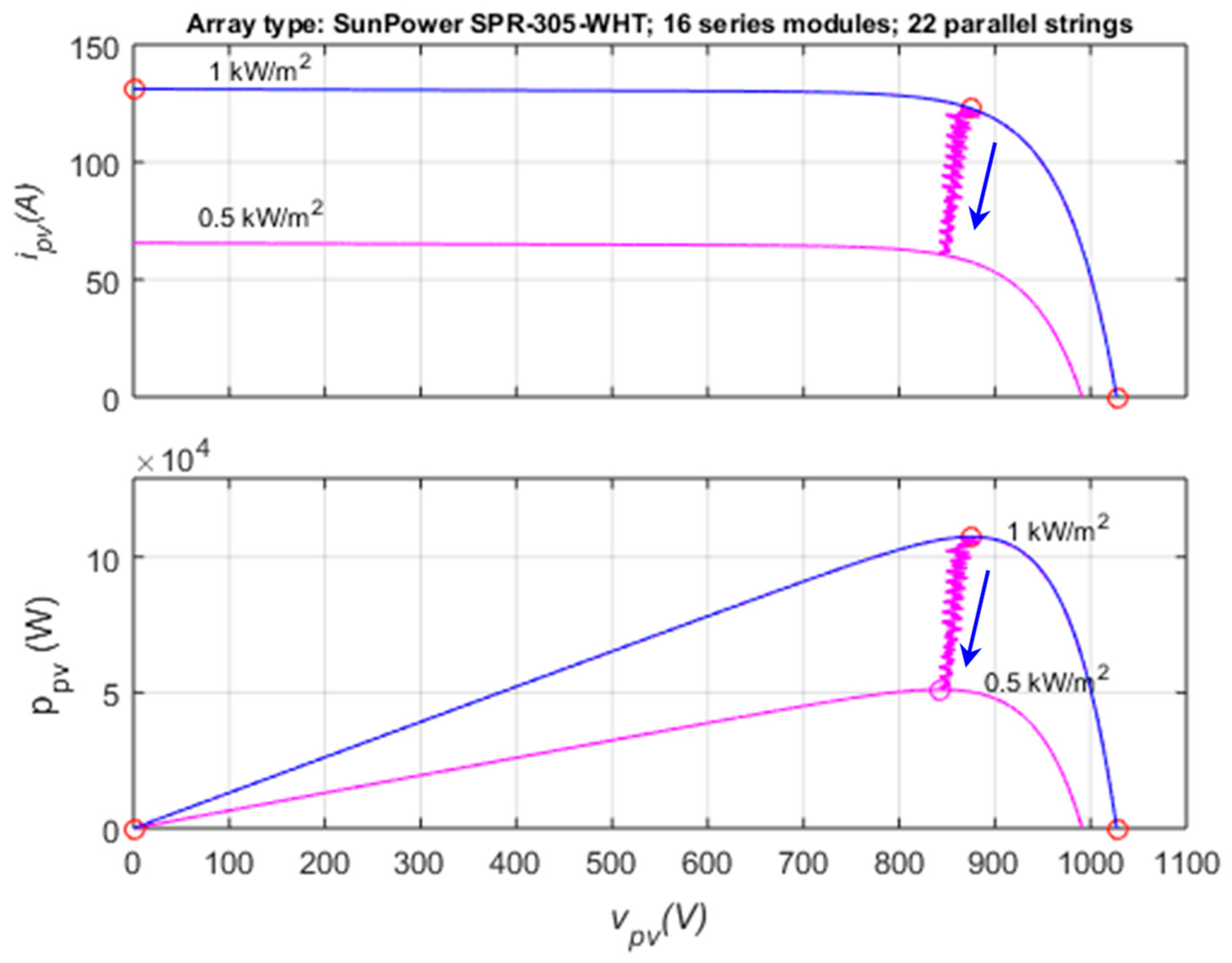
5. Simulation Results

In order to validate the proposed analysis, the three-phase grid-connected PV generation system shown in Figure 1 was simulated in Matlab-Simulink. The circuit parameters are summarized in Table 1. A string of series/parallel connected PV modules has been adopted as PV source, according to the data given in Table 2 in standard test conditions (STC). In particular, the considered PV modules are SP-305 type (96 cells, monocrystalline).
The first simulation test is carried out in order to verify the input/output steady-state waveforms of the PV generation system with considered three-phase three-level FC inverter.
In particular, Figure 9 shows grid voltage and current (top traces), PV voltage (medium trace) and PV current (bottom trace). It can be noticed that the grid current is almost sinusoidal, with unity power factor. As expected, the PV voltage and PV current have 3rd harmonic component oscillations (150 Hz), in phase opposition. The proposed RCC-MPPT algorithm can well track the maximum power point at sun irradiance E = 1000 W/m2 (in this case Vmpp = 875 V and Impp = 123 A).
The following simulation tests are carried out to verify the dynamic performance of the proposed RCC-MPPT algorithm in case of fast solar irradiance transients. In particular, two scenarios have been considered:
  • Sun irradiance (ramp) increase,
  • Sun irradiance (ramp) decrease.
The cell temperature has been considered constant (25 °C) during simulations for both scenarios.
The simulation results depicted in Figure 10 and Figure 11 show the behavior of the considered system during the first scenario. A linear ramp increase of solar irradiance from 500 W/m2 to 1000 W/m2 is applied in a transient period of 200 ms, between 1.3 s and 1.5 s. The results clearly indicate that as soon as the transient occurs, the estimation of dPpv/dVpv is oscillating. However, it is almost acceptable during the steady-state (Figure 10b), which means that the PV current and the PV voltage perfectly follow the MPP under this kind of smooth irradiance change (Figure 10c,d). Figure 10e presents the waveform of the injected grid current. The injected grid current is perfectly sinusoidal and well controlled thanks to the dynamic performance of the dq current controller.
Figure 11 shows the Ppv(Vpv) and Ipv(Vpv) diagrams corresponding to the transient depicted in Figure 10. The operating point moves from the first MPP, before the solar irradiance transient, to the new MPP, in the steady-state condition after the transient.
Simulation results for ramp decrease in solar irradiance are presented in Figure 12 and Figure 13. In this case, the initial value of solar irradiance is 1000 W/m2, decreasing linearly to 500 W/m2 in a period of 200 ms. As can be seen, the estimation of dPpv/dVpv is correct during the steady state (Figure 12b). At the end of the transient, the estimation of dPpv/dVpv becomes correct again, and the operating point is correctly driven toward the MPP. The current injected into the grid is perfectly sinusoidal and follows the sun irradiance profile (Figure 12e). The path of the operating points is displayed on the Ppv(Vpv) and Ipv(Vpv) diagrams and presented in Figure 13.

6. Conclusions

In this paper, an original RCC-MPPT algorithm suitable for three-phase three-level flying capacitor photovoltaic systems has been proposed and analyzed in detail. The three-phase FC inverter introduces voltage and current harmonics on the input (i.e., PV) side. In particular, a significant 3rd order harmonic is clearly noticeable, whereas higher harmonic components have much lower amplitudes. Both PV voltage and current harmonic amplitudes are analytically calculated in the whole modulation range in case of centered PWM, offering the possibility of a precise and effective design of the DC-link capacitor in order to obtain the desired ripple amplitude.
Because of the presence of different harmonics, a ripple correlation control scheme extracting the amplitude of a specific harmonic from PV voltage and current waveforms has been proposed in order to track the maximum power point of the PV arrays. Specifically, the estimation of dIpv/dVpv (and then dPpv/dVpv) is carried out by considering the 3rd order harmonic of PV voltage and current oscillations.
Numerical tests have been performed to prove the effectiveness of the whole PV generation scheme, including three-phase three-level FC inverter and the proposed RCC-MPPT algorithm. Tests have been carried out considering both steady-state conditions and fast solar irradiance transients in order to verify the dynamic performance of the proposed RCC algorithm, resulting in an effective and original MPPT method in the case of three-phase PV systems.

Author Contributions

M.H. and G.G. developed the theoretical analysis; M.H. performed the simulation results, also providing for the manuscript arrangement in cooperation with M.R.; A.R. and G.G. generally supervised and finalized the work.

Funding

This research received no external funding.

Conflicts of Interest

The authors declare no conflict of interest.

References

  1. Elgendy, M.A.; Zahawi, B.; Atkinson, D.J. Assessment of Perturb and Observe MPPPT Algorithm Implementaion Techniques for PV Pumping Applications. IEEE Trans. Sustain. Energy 2012, 3, 21–33. [Google Scholar] [CrossRef]
  2. Kumar, N.; Hussain, I.; Singh, B.; Panigrahi, B.K. Self-Adaptive Incremental Conductance Algorithm for Swift and Ripple-Free Maximum Power Harvesting from PV Array. IEEE Trans. Ind. Inform. 2018, 14, 2031–2041. [Google Scholar] [CrossRef]
  3. Thangavelu, A.; Vairakannu, S.; Parvathyshankar, D. Linear Open Circuit Voltage-Variable Step-Size-Incremental Conductance Strategy-Based Hybrid MPPT Controller for Remote Power Applications. IET Power Electron. 2017, 10, 1363–1376. [Google Scholar] [CrossRef]
  4. Ariyur, K.; Krstic, M. Real-Time Optimization by Extremum-Seeking Control; Wiley: Howard, NY, USA, 2003. [Google Scholar]
  5. Ghaffari, A.; Seshagiri, S.; Krstic, M. Control Engineering Practice Multivariable Maximum Power Point Tracking for Photovoltaic Micro-Converters Using Extremum Seeking. Control Eng. Pract. 2015, 35, 83–91. [Google Scholar] [CrossRef]
  6. Ghaffari, A.; Krstic, M.; Seshagiri, S. Power Optimization for Photovoltaic Microconverters Using Multivariable Newton-Based Extremum Seeking. IEEE Trans. Control Syst. Technol. 2014, 22, 2141–2149. [Google Scholar] [CrossRef]
  7. Barth, C.; Pilawa-Podgurski, R.C.N. Dithering Digital Ripple Correlation Control for Photovoltaic Maximum Power Point Tracking. IEEE Trans. Power Electron. 2015, 30, 4548–4559. [Google Scholar] [CrossRef]
  8. Kimball, J.W.; Krein, P.T. Discrete-Time Ripple Correlation Control for Maximum Power Point Tracking. IEEE Trans. Power Electron. 2008, 23, 2353–2362. [Google Scholar] [CrossRef]
  9. Bazzi, A.M.; Krein, P.T. Ripple Correlation Control: An Extremum Seeking Control Perspective for Real-Time Optimization. IEEE Trans. Power Electron. 2014, 29, 988–995. [Google Scholar] [CrossRef]
  10. Hammami, M.; Grandi, G. A Single-Phase Multilevel PV Generation System with an Improved Ripple Correlation Control. Energies 2017, 10, 2037. [Google Scholar] [CrossRef]
  11. Hammami, M.; Grandi, G.; Rudan, M. RCC-MPPT Algorithms for Single-Phase PV Systems in Case of Multiple DC Harmonics. In Proceedings of the 6th International Conference on Clean Electrical Power (ICCEP), Santa Margherita Ligure, Italy, 27–29 June 2017. [Google Scholar]
  12. Casadei, D.; Grandi, G.; Rossi, C. Single-Phase Single-Stage Photovoltaic Generation System Based on a Ripple Correlation Control Maximum Power Point Tracking. IEEE Trans. Energy Convers. 2006, 21, 562–568. [Google Scholar] [CrossRef]
  13. Hammami, M.; Grandi, G.; Rudan, M. An Improved MPPT Algorithm Based on Hybrid RCC Scheme for Single-Phase PV Systems. In Proceedings of the 42nd Annual Conference of the IEEE Industrial Electronics Society (IECON), Florence, Italy, 23–26 October 2016. [Google Scholar]
  14. Esram, T.; Kimball, J.W.; Krein, P.T.; Chapman, P.L.; Midya, P. Dynamic Maximum Power Point Tracking of Photovoltaic Arrays Using Ripple Correlation Control. IEEE Trans. Power Electron. 2006, 21, 1282–1290. [Google Scholar] [CrossRef]
  15. Elnosh, A.; Khadkikar, V.; Xiao, W.; James, L. An Improved Extremum—Seeking Based MPPT for Grid—Connected PV Systems with Partial Shading. In Proceedings of the 2014 IEEE 23rd International Symposium on Industrial Electronics (ISIE), Istanbul, Turkey, 1–4 June 2014. [Google Scholar]
  16. Yuan, X.; Stemmler, H.; Barbi, I. Self-Balancing of the Clamping-Capacitor-Voltages in the Multilevel Capacitor-Clamping-Inverter under Sub-Harmonic PWM Modulation. IEEE Trans. Power Electron. 2001, 16, 256–263. [Google Scholar]
  17. Babaei, E.; Laali, S.; Bayat, Z. A Single-Phase Cascaded Multilevel Inverter Based on a New Basic Unit with Reduced Number of Power Switches. IEEE Trans. Ind. Electron. 2015, 62, 922–929. [Google Scholar] [CrossRef]
  18. Buticchi, G.; Barater, D.; Lorenzani, E.; Concari, C.; Franceschini, G. A Nine-Level Grid-Connected Converter Topology for Single-Phase Transformerless PV Systems. IEEE Trans. Ind. Electron. 2014, 61, 3951–3960. [Google Scholar] [CrossRef]
  19. Rahim, N.A.; Selvaraj, J. Multistring Five-Level Inverter with Novel PWM Control Scheme for PV Application. IEEE Trans. Ind. Electron. 2010, 57, 2111–2123. [Google Scholar] [CrossRef]
  20. Hammami, M.; Rizzoli, G.; Mandrioli, R.; Grandi, G. Capacitors Voltage Switching Ripple in Three-Phase Three-Level Neutral Point Clamped Inverters With. Energies 2018, 11, 3244. [Google Scholar] [CrossRef]
  21. Hammami, M.; Vujacic, M.; Grandi, G. Dc-Link Current and Voltage Ripple Harmonics in Three-Phase Three-Level Flying Capacitor Inverters with Sinusoidal Carrier-Based PWM. In Proceedings of the 19th International Conference on Imdustrial Technology (ICIT), Lyon, France, 20–22 February 2018. [Google Scholar]
  22. Nabae, A.; Takahashi, I.; Akagi, H. A New Neutral-Point-Clamped PWM Inverter. IEEE Trans. Ind. Appl. 1981, IA-17, 518–523. [Google Scholar] [CrossRef]
  23. Margaliot, M.; Ruderman, A.; Reznikov, B. Mathematical Analysis of a Flying Capacitor Converter: A Sampled- Data Modeling Approach. Int. J. Circuit Therory Appl. 2013, 41, 682–700. [Google Scholar] [CrossRef]
  24. Ibrayeva, A.; Ten, V.; Familiant, Y.L.; Ruderman, A. PWM Strategy for Improved Natural Balancing of a Four-Level H-Bridge Flying Capacitor Converter. In Proceedings of the Aegean Conference on Electrical Machines and Power Electroonics (ACEMP), Side, Turkey, 2–4 September 2015. [Google Scholar]
  25. Thielemans, S.; Ruderman, A.; Reznikov, B. Improved Natural Balancing With Modified Phase-Shifted PWM for Single-Leg Five-Level Flying-Capacitor Converters. IEEE Trans. Power Electron. 2012, 27, 1658–1667. [Google Scholar] [CrossRef] [Green Version]
Figure 1. Three-phase grid-connected PV generation system based on three-level FC inverter.
Electronics 08 00118 g001
Figure 2. Carrier-based CPWM modulation logic for each leg (i) of three-level FC inverter in case of m = 0.577/2 (red trace), m = 0.43 (green trace) and m = 0.577 (blue trace). Underline denotes complementary.
Electronics 08 00118 g002
Figure 3. One leg input current (top) and total inverter input current (bottom): instantaneous value (blue trace), its numerically averaged value over the switching period (red), and theoretical value (green) in case of for m = 0.577/2 and m = 0.577 (from right to left), Iac = 1 A and φ = 0°.
Electronics 08 00118 g003
Figure 4. Alternating PV voltage ripple (green trace) and its averaged value over the switching period (pink trace), for m = 0.577/2 (left) and m = 0.577 (right), Iac/wC = 1.
Electronics 08 00118 g004
Figure 5. Alternating PV current ripple (red trace) and its averaged value over the switching period (blue trace), for m = 0.577/2 (left) and m = 0.577 (right), Iac/wC = 1 and Rpv = 7.13 Ω.
Electronics 08 00118 g005
Figure 6. Control scheme of the PV generation system.
Electronics 08 00118 g006
Figure 7. Simulation example of: (a) grid current and inverter output voltage, (b) PV voltage, and (c) PV current, in case of three-phase flying capacitor inverter.
Electronics 08 00118 g007
Figure 8. Block diagram of proposed RCC, estimating dPpv/dVpv by the 3rd harmonic component.
Electronics 08 00118 g008
Figure 9. Input/output steady-state waveforms of the FC in case of sun irradiance E = 1000 W/m2: grid voltage and current (top traces), PV voltage (middle trace) and PV current (bottom trace).
Electronics 08 00118 g009
Figure 10. Irradiance ramp increase: (a) irradiance, (b) power derivative, (c) photovoltaic current. (d) photovoltaic voltage, and (e) grid current, in case of proposed RCC-MPPT algorithm.
Electronics 08 00118 g010
Figure 11. Effects of a 50% irradiance transient of PV power vs. PV voltage in case of irradiance ramp decrease.
Electronics 08 00118 g011
Figure 12. Irradiance ramp decrease: (a) irradiance, (b) power derivative, (c) photovoltaic current, (d) photovoltaic voltage, and (e) grid current, in case of proposed RCC-MPPT algorithm.
Electronics 08 00118 g012
Figure 13. Effects of a 50% irradiance transient of PV power vs. PV voltage in case of irradiance ramp decrease.
Electronics 08 00118 g013
Table 1. Simulation circuit parameters.
LabelDescriptionParameters
VacGrid voltage (rms)230 V
Lf, RfAc-link inductor1 mH, 3 mΩ
CDC-link capacitor2 mF
CA, CB, CCFlying capacitors5 mF
f, fswFundamental and switching frequencies50 Hz, 3kHz
Table 2. PV module specifications (STC) and modules arrangement.
LabelDescriptionParameters
VOCOpen circuit voltage64.2 V
ISCShort circuit current5.96 A
VmppMaximum photovoltaic voltage54.7 V
ImppMaximum photovoltaic current5.58 A
NSNumber of series-connected modules per string16
NPNumber of parallel strings22

