A Feature Integrated Saliency Estimation Model for Omnidirectional Immersive Images

Abstract

Omnidirectional, or 360°, cameras are able to capture the surrounding space, thus providing an immersive experience when the acquired data is viewed using head mounted displays. Such an immersive experience inherently generates an illusion of being in a virtual environment. The popularity of 360° media has been growing in recent years. However, due to the large amount of data, processing and transmission pose several challenges. To this aim, efforts are being devoted to the identification of regions that can be used for compressing 360° images while guaranteeing the immersive feeling. In this contribution, we present a saliency estimation model that considers the spherical properties of the images. The proposed approach first divides the 360° image into multiple patches that replicate the positions (viewports) looked at by a subject while viewing a 360° image using a head mounted display. Next, a set of low-level features able to depict various properties of an image scene is extracted from each patch. The extracted features are combined to estimate the 360° saliency map. Finally, bias induced during image exploration and illumination variation is fine-tuned for estimating the final saliency map. The proposed method is evaluated using a benchmark 360° image dataset and is compared with two baselines and eight state-of-the-art approaches for saliency estimation. The obtained results show that the proposed model outperforms existing saliency estimation models.

1. Introduction

In the last decade we have witnessed significant development in multimedia technologies. This includes media acquisition devices, rendering systems, compression techniques, and application scenarios. Omnidirectional or 360° imaging allows to record a complete scene from a specific point of view. The acquired information can be rendered through a Head Mounted Display (HMD) thus providing an immersive experience to the user. To allow the adoption of this technology, many challenges need to be solved: Understanding the degree of appreciation of users, evaluating the impact of transmission noise or processing artifacts, or even the most suitable way for rendering 360° media.

The focus of our research is to study the exploring behavior of a 360° content by a user using HMDs. As known in psycho-physiology, humans browse a scene according to its saliency. At each glance, the human vision system analyzes the input and fixates the attention on prominent aspects of a scene. The study of saliency can be exploited for several applications such as compression [1], health monitoring systems [2,3,4], or marketing [5].

The models developed for saliency estimation try to emulate the HVS mechanisms by exploiting cognition, machine learning, statistical analysis, neuroscience, and computer vision. The first approaches towards the saliency estimation rely on the detection of image components attracting human attention, i.e., color, intensity, and texture [6,7].

Other approaches exploit Gestalt’s psychological studies [8,9], according to which human perception focuses on figures more than on background elements. In [10] a Boolean map based saliency model (BMS) for 2D images is presented and an extended version of this approach, the extended Boolean map saliency approach (EBMS), is proposed in [11].

Both BMS and EBMS do not consider the geometry-related features of an image and cannot directly be used for omnidirectional content since they do not address the problem of spherical projection of 360° images that may cause artifacts. Fang et al. [12] adapt the traditional 2D saliency approach to 360° images. Other methods adopt low-level features [12,13] or a combination of low and high-level features [14,15,16] for 360° image saliency estimation.

Recently, methods have been proposed to take into account the artifacts caused by the spherical projections. In [17], performances of three saliency estimation methods: Graph-based visual saliency, ensemble of deep networks (eDN), and the saliency attentive model (SAM) are compared. eDN exploits a six-multilayer structure to identify the salient regions through hyper-parameter optimisation. The ResNet architecture combined with pre-trained VGG-16 is used in the SAM model. Each model is tested using three types of 360° image projection formats: Continuity, cube, and combined equirectangular image projection.

Low-level and high-level features are combined in [14]. Low-level features include hue, saturation, texture and graph-based visual saliency (GBVS) [7] on the hue component. Number of persons, skin color, and faces are considered as high-level features. A superpixel-based saliency estimation model, exploiting contrast and boundary connectivity, is proposed in [12]. Biswas et al. [13] pre-process the 360° images before applying the Itti [6] and GBVS [7] models for saliency estimation. Pre-processing includes illumination normalization. This step is important since, due to the spherical aspect of the scene, the lighting is not uniformly distributed. Therefore, if the gaze of the observer falls between bright and dark areas, the bright areas will be more attractive than the dark ones. However, if the user gazes towards comparatively dark regions, objects in those regions will be of higher importance due to the lightness adaptation. In addition to the high and low-level image features, it has been observed that the content of an image drives visual attention. In this direction, in [15] the importance of objects present in an image for saliency estimation is addressed. Zhu et al. [16] perform saliency estimation of 360° images using head movement data of subjects wearing HMD. Projection of 360° images usually generates artifacts near the periphery. To reduce this artifact, in [16] a pseudo-cylindrical projection [18] is performed instead of the popular equirectangular projection.

In this paper, a Feature Integrated 360° image Saliency Estimation Model (FISEM) is proposed. The novelties introduced with respect to the state-of-the-art are:

• We primarily focus on the geometry-based features of an image. It has been observed in many studies that the geometry of the physical world helps in visual perception of a scene [19,20]. Taking this into consideration, we extract a set of image features that depicts the geometry of an image stimuli. In addition, artifacts caused by spherical projections of a 360° image are taken into account;
• the illumination effects are normalized before extracting the geometry-based features [13]. The human retina can adjust to various levels of light [21] and non-uniform luminance has a large impact on human visual perception [22], and consequently on saliency estimation [13,23];
• the image foreground is considered as a feature. Human perception is highly influenced by objects located in the foreground regions [9]. Therefore, we perform a foreground/background separation. To the best of our knowledge this is the first approach that exploits image foreground as a feature for saliency estimation of omnidirectional images.

The rest of the paper is organized as follows: In Section 2 the proposed saliency model is described. Section 3 reports the results of performed tests and finally Section 4 draws the conclusions.

2. Proposed Methodology

The proposed approach consists of pre-processing, image features extraction and integration, and post-processing (as shown in Figure 1).

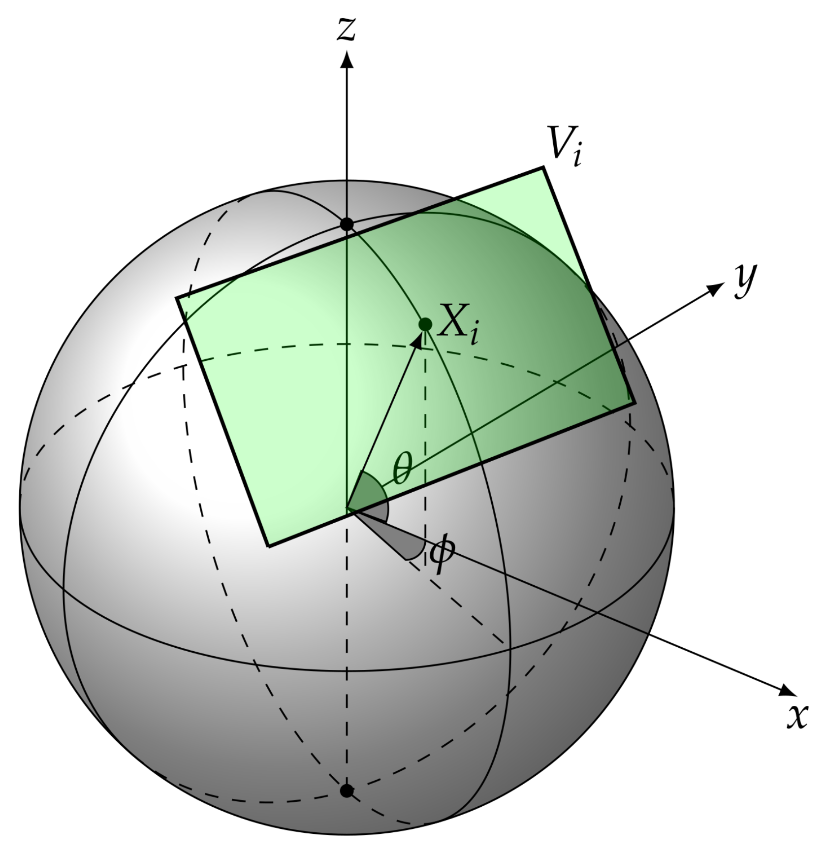
2.1. Viewport Extraction

HMDs are currently mostly used to display 360° media. They provide a fixed field-of-view (FOV) thus showing a windowed view of the image content and not the entire image as a whole. Thus, while using a HMD, users need to move their head for exploring the image content. Each 360° image is therefore explored by means of small windows which are known as ‘viewports’. As the target of saliency estimation is to understand where a user looks within the image, it is necessary to simulate the viewing windows or viewports. To this aim, multiple projection techniques are available, such as equirectangular, cube-map, truncated square-pyramid, craster parabolic, or equal area projection [24,25]. Since the equirectangular projection results in a less noisy and geometrically distorted representation, it has been widely adopted [16]. In this work we apply the equirectangular projection [14], briefly reported in the following for sake of clarity.

A non-uniform angular sampling is performed over the omnidirectional image. The sampled points are represented as $X_i$, where i refers to the number of points. It can be noted that the number of sampled coordinates $X_i$ corresponds to the number of viewports extracted from one single 360° image. Moreover, the centre of viewport is fixed at the sampled point $X_i$ with a fixed width and height. Therefore, the set of viewports V is $(1,2,\dots ,X_i)$. Each pixel in the considered viewport is further projected to the rectilinear plane (gnomonic projection). In this regard, a 3D Cartesian coordinate system is used, having its origin surrounded by a spherical frame of fixed radius. Let $M_{V_i}$ be any point with co-ordinates $(x,y)$ in the viewport $V_i$ in V. Each point is placed on the plane tangent to the sampled point $X_i$. This process is depicted in Figure 2. The 3D Cartesian coordinate system position of $M_{V_i}$ in the rectilinear plane is computed as

$$M_{V_i}^{pos}\left(x,y,z\right)=\left\{\begin{array}{cc}x:& 1\\ y:& px·\left(x-\frac{V_{width}}{2}\right)\\ z:& px·\left(y-\frac{V_{height}}{2}\right)\end{array}\right\}$$

(1)

where $px$ is the pixel intensity, and $V_{width}$, $V_{height}$ are the fixed width and height of the generated viewports. The point $M_{V_i}$ is projected to the rectilinear plane as

$$M_{V_i}^{proj}=\frac{M_{V_i}^{pos}\left(x,y,z\right)}{∥M_{V_i}^{pos}\left(x,y,z\right)∥}$$

(2)

where $∥·∥$ denotes the $L^2$-norm of $M_{V_i}^{pos}$. The projected viewports for each 360° image are processed individually, as explained in the following subsections.

2.2. Illumination Normalization

In order to perform illumination normalization, we first analyse how the pixel intensities vary in each viewport $V_i$. To this aim, each viewport is processed to extract its average pixel weight ($vAPW$). Then, the global average pixel weight ($gAPW$) of the entire omnidirectional image is determined as the mean of $vAPWs$ values computed for all the viewports V

$$gAPW=\sum _{i=1}^n\frac{vAP{W}_i}{n}$$

(3)

where n is the number of viewports and $vAP{W}_i$ is the average pixel weight for the viewport i.

Here, we distinguish the viewports into three categories: Over illuminated ($vAPW>gAPW$), nearly uniform illuminated ($\frac{gAPW}{2}<vAPW<gAPW$) and under illuminated (Figure 3). In order to normalize the illumination within the viewport we process the over and under illuminated viewports.

The contrast of an image can be controlled by using histogram equalization (HE) [26]. To cope with over illuminated regions, the histogram equalized viewport $V_i$ is further processed with a DWT based normalization technique. In particular, a second level DWT is performed and the LL subband is processed by subtracting 2/3 of the mean pixel weight of 2D viewport image. The algorithm for illumination normalization of both over and under illuminated images is provided in (Algorithm 1). The illumination normalized image obtained from the HDWT algorithm and low light image enhancement algorithm is shown in Figure 4.

Algorithm 1: HDWT: Illumination Normalization

2.3. Feature Extraction

A set of independent low-level features are extracted from viewports: Color, contrast, orientation, intensity, edge, ridge, shape, and corner. The extracted features are described in the following

• Color (${\mathit{V}}_{\mathit{i}}^{\mathit{C}}$), Intensity (${\mathit{V}}_{\mathit{i}}^{\mathit{Int}}$) and Contrast (${\mathit{V}}_{\mathit{i}}^{\mathit{Cnt}}$): first we convert the RGB viewport ($V_i$) into the CIE$Lab$ color space to find the three components: Lightness (L), color weight between green and red channels (a) and color weight between blue and yellow channels (b). We compute $V_i^C$ as the average value of the L, a and b components

  $$V_i^C=\frac{L+a+b}{3}.$$
  The viewport image intensity map $V_i^{Int}$ is generated in two steps. First, the highest pixel value along the three components L, a and b is considered for generating a preliminary intensity map $V_i^{pim}$. Second, Prewitt gradient operator is used to generate the gradient map of the intensity image

  $$V_i^{Int}=Prewitt\left(V_i^{pim}\right).$$
  Variation in image contrast affects human visual perception [27]. We accounted for this aspect by using as feature a gray level map obtained from a contrast enhanced version of the viewport $V_i$. The contrast enhancement is performed by saturating the bottom $20\%$ and the top 30% of all pixel values:

  $$V_i^{Cnt}=Ou{t}_{low}+(Ou{t}_{low}-Ou{t}_{high})\ast \frac{V_i-V_i\left(low\right)}{V_i\left(high\right)-V_i\left(low\right)}$$

  where $V_i\left(low\right)$ and $V_i\left(high\right)$ are the smallest and the largest pixel values in $V_i$, and $Ou{t}_{low}$ and $Ou{t}_{high}$ are, respectively, the $20\%$ of $V_i\left(low\right)$ and the $30\%$ of $V_i\left(high\right)$.
• Edge (${\mathit{V}}_{\mathit{i}}^{\mathit{Edg}}$): The Canny edge detector [28] is adopted for identifying the horizontal and vertical edges in an image

  $$V_i^{Edg}=Canny\left(V_i\right).$$
• Corner (${\mathit{V}}_{\mathit{i}}^{\mathit{Cor}}$): Corners are regions in which we observe a very high variation in intensity in all directions. Therefore we apply the Harris corner detector [29] which is robust to illumination, rotation, and translation.
• Ridge (${\mathit{V}}_{\mathit{i}}^{\mathit{Rid}}$): As multiple objects reside in an image scene, ridge ending and bifurcations (Figure 5) can be a significant feature source for saliency estimation since they allow to detect points in the image when a change happens. In this work we adopt the ridge extraction technique proposed in [30]. The viewport image is first binarized and subsequently, a morphology-based thinning operation is performed.
• Shape (${\mathit{V}}_{\mathit{i}}^{\mathit{Hou}}$): The Hough transform [32] is used for detecting regular shapes such as lines, circles and centroid points [33] of connected objects.
• Orientation (${\mathit{V}}_{\mathit{i}}^{\mathit{Ori}}$): In order to extract information on orientation we follow the approaches based on Gabor filtering as suggested in [34,35].

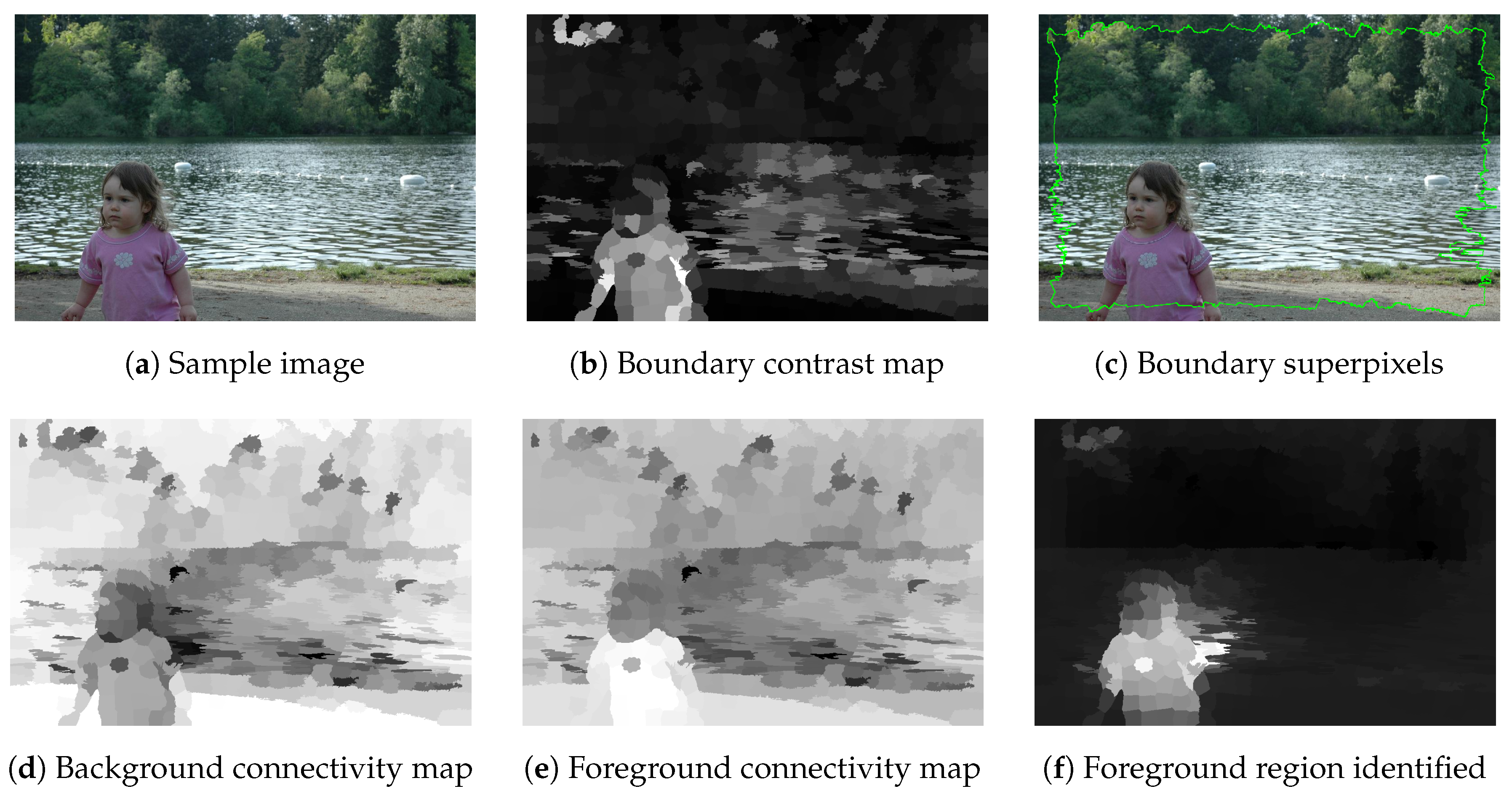
2.4. Foreground Extraction

As stated in the Introduction, human perception is highly influenced by the objects located in the foreground regions [9]. Based on this evidence, we extract the foreground of an image and use it as feature. The graph-based foreground/background extraction approach proposed in [36] is adopted.

A region is classified as foreground according to two factors: Distance from image boundary and distance from local neighbourhood. A superpixel-based SLIC segmentation [37] is performed on the viewport image. An optimization framework [38] is used for combining the foreground and background connectivity maps by considering three constraints:

• Superpixels with large values in the foreground map are salient;
• superpixels with large values in the background map are non-salient;
• superpixels that are similar and adjacent should have the same saliency values.

We extract the pixels marked as foreground and assign to them the highest pixel intensity. Pixels considered as belonging to the background, are set at the lowest intensity. All pixel intensities are then normalized between 0 and 1 to obtain the final foreground map $V_i^{Fore}$. Figure 6 depicts the steps described above.

2.5. Feature Integration

Low-level image features are combined for generating the saliency maps for each viewport. In more details: A linear combination of color, intensity, contrast, edge, corner, ridge, shape, and orientation is performed to generate the low-level feature map $V_i^{LFM}$

$$V_i^{LFM}=V_i^C+V_i^{Int}+V_i^{Cnt}+V_i^{Edg}+V_i^{Cor}+V_i^{Rid}+V_i^{Hou}+V_i^{Ori}.$$

(4)

Then, the maximum pixel value between $V_i^{LFM}$ and the foreground map $V_i^{Fore}$ is selected as weight of the final viewport saliency map $Sa{l}_{V_i}$

$$Sa{l}_{V_i}=maximum(V_i^{LFM},V_i^{Fore}).$$

(5)

Following the approach adopted in [14], the saliency maps of each viewport are re-projected to a single equirectangular saliency map for further processing and comparison with the ground truth. Coordinates for the equirectangular saliency map are computed as

$$Sa{l}_{equirect}(x,y)=\left\{\begin{array}{cc}x:& I_{width}·\left({\displaystyle \frac{ang}{2\pi }}\right)\\ y:& I_{height}·\left({\displaystyle \frac{arcsin\left(M_{V_i}^{proj}\left(z\right)\right)}{\pi +0.5}}\right)\end{array}\right\}$$

(6)

where, $I_{width}$, $I_{height}$ are the input 360° image width and height, respectively, and $ang$ is computed from the four-quadrant tangent function as $ta{n}^{-1}(M_{V_i}^{proj}\left(x\right),M_{{V_i}^{proj}}\left(y\right))$.

2.6. Post-Processing

To cope with the fact that users tend to concentrate more on the equator region of a 360° image, the proposed approach gives highest weight to equator pixels, to obtain $I_{equibias}$. To this aim, a Laplacian fitting approach based on probability density function [40] is used to compute pixel weight of the input 360° image. Then, the equator biased saliency map $Sa{l}_{equibias}$ is computed as

$$Sa{l}_{equibias}=Sa{l}_{equirect}+I_{equibias}.$$

(7)

To control the impact of illumination on $Sa{l}_{equibias}$, we utilise the anisotropic diffusion technique [41]. It is applied to the luminance component of the input 360° image to generate a binarized image $I_{bin}$. The zero pixels in $I_{bin}$ represent the low illuminated regions. They are modified by performing the average of $[3\times 3]$ neighbourhood in $I_{bin}$ and the resultant binary image is $I_{bin}$’. After this operation, there will still be 0-valued pixels in $I_{bin}$’ and they need to be normalized. Therefore, the pixels in $Sa{l}_{equibias}$ that correspond to the 0 pixel locations in $I_{bin}$’ are selected for illumination normalization as

$$Sa{l}_{final}(x,y)=\left\{\begin{array}{cc}Sa{l}_{equibias}(x,y)& if{I}_{bin}^{\prime }(x,y)=1\\ 0.6\ast Sa{l}_{equibias}(x,y)& if{I}_{bin}^{\prime }(x,y)=0\end{array}\right\}$$

(8)

$Sa{l}_{final}$ is the final estimated 360° saliency map for the proposed model FISEM.

3. Experimental Results

The proposed FISEM model is evaluated by using the Salient360! [42] head only dataset. The dataset consists of 85 omnidirectional images and their corresponding ground truth saliency maps. For performance evaluation we select the Correlation Coefficient (CC) and Kullback–Leibler Divergence (KLD) metrics. CC evaluates the statistical relationship between two saliency maps (estimated and ground truth). A higher correlation depicts better estimation of saliency. The KLD measures the deviation of probability distribution of the estimated image and the available ground truth. A lower KLD indicates better saliency estimation. As per the saliency benchmarks [43], these two metrics (CC and KLD) are the standard metrics used for evaluating head movement based saliency models. The proposed FISEM is compared with two baseline saliency estimation models: Boolean map saliency (BMS) [10] and extended Boolean map saliency (EBMS) [11]. Furthermore, we compare our approach with eight existing state-of-the-art 360° image saliency estimation approaches: SJTU [16], COSE [15], RM3 [14], JU [12], LCSP [13], and TU1, TU2, and TU3 [17].

FISEM is implemented in a 3.3 GHz quad-core 64-bit Windows 10 desktop machine with 8 GB memory. Matlab platform is used for programming the FISEM saliency model. The dimension of the 360° images in Salient360! dataset ranges from $910\times 450$ pixels to $18264\times 9132$ pixels. All the images in Salient360! were resized to $1920\times 1080$ pixels and used in the FISEM model. The proposed model takes a total of 22 minutes to estimate saliency map of a $1920\times 1080$ pixels 360° image.

The HMD used for generating the dataset in [42] had field-of-view (FOV) of 100° and resolution of $960\times 1080$ pixels. Therefore, for generating viewports for each 360° image we set resolution of 1920 × 1080 pixels (see Section 2.1). The Laplacian curve fitting used for incorporating equator bias needs two parameters. The scale parameter that depicts diversity is set at 15 and the location parameter defined as a latitude while viewing image in head mounted displays is set at 90. For the Salient360! dataset, the global average pixel weight ($gAPW$) is obtained at 106.

Experimental Results and Analysis

The experimental results are depicted in

Table 1. (a) Performance comparison averaged on the images in the dataset [42]. (b) and (c) are the best and worst performing images with the feature integrated 360° image saliency estimation model (FISEM) approach, respectively.

(a) Results on the test dataset.
Model		CC↑	KLD↓
FISEM		0.69	0.47
SJTU [16]		0.67	0.65
COSE [15]		0.65	0.72
TU1 [17]		0.62	0.75
TU2 [17]		0.56	0.64
EBMS [11]		0.57	0.8
RM3 [14]		0.52	0.81
JU [12]		0.57	1.14
BMS [10]		0.51	0.94
LCSP [13]		0.43	0.78
TU3 [17]		0.44	1.09
(b) Best performing images.
Metric	P28	P76	P95	P85
CC	0.87	0.83	0.83	0.82
KLD	0.26	0.37	0.47	0.32
Metric	P27	P28	P17	P35
KLD	0.23	0.26	0.27	0.28
CC	0.66	0.87	0.67	0.77
(c) Worst performing images.
Metric	P15	P10	P23	P31
CC	0.11	0.42	0.46	0.49
KLD	0.96	0.64	0.75	0.34
Metric	P33	P4	P64	P43
KLD	2.22	1.84	1.40	1.19
CC	0.67	0.62	0.6	0.68

. In Table 1a the average value of CC and KLD over all the 85 omnidirectional images are presented for our approach and the compared approaches. Table 1b,c showcases the best and worst performing images in the Salient360! dataset for the proposed model FISEM.

BMS and EBMS are the two baseline models for estimating saliency in 2D images; therefore, their approaches do not consider the peculiarities of a 360° image, such as projection artifacts, attention bias, etc. However, for performance comparison with these baselines on the 360° images, we adapted the BMS and EBMS algorithms to work for 360° images. We perform equirectangular projection for extracting viewports and subsequently, apply the standard BMS/EBMS on the viewports. It can be noted that FISEM uses equirectangular projection; therefore, for the sake of comparison we choose this projection technique for implementing BMS and EBMS on the Salient360! dataset. The BMS approach obtained CC and KLD of 0.51 and 0.94, respectively, whereas, the EBMS produced much improved results of 0.57 (CC) and 0.8 (KLD) for the Salient360! dataset. However, both BMS and EBMS approach underperform for 360° images when compared with our proposed approach.

Next we analyse performance of state-of-the-art algorithms in 360° saliency estimation with respect to the proposed FISEM and we have analysed the best and worst performing images. Table 1b shows the best performing images in Salient360! using our proposed FISEM approach. We selected the top four images with the highest CC and the top four images showing the lowest KLD. Similarly, Table 1c shows the worst performing images both in terms of CC and KLD values. The original images, ground truth saliency maps, and the estimated saliency maps using FISEM for all the best and worst performing images are shown in Figure 7 and Figure 8, respectively.

It can be observed that the uniform distribution of luminance and presence of identical image texture affects the performances of the proposed method. For example, images 27 and 28 are uniformly illuminated. Generally an omnidirectional image is affected by a series of distortions, starting from image capture to rendering in the head mounted displays [44]. Our analysis on the performance of FISEM reveals that the least geometrically distorted images performed better with FISEM. For example, images such as 4, 10, and 64 are very distorted and such geometric distortions near to the periphery affect overall saliency estimation. Along with the distortion artefacts we also observed that saliency is driven by the content depicted in the image. For reference, in images 15, 33, and 43 the subjects mostly focus their attention towards a particular region of the image, even though they had the possibility of free exploration of the entire content.

Interestingly, in these three images (15, 33, and 43) it can be noticed that the most salient regions (with respect to ground truths) do not have any particular interesting or unique object that could attract attention. Therefore, the possibility of performing an object detection and using it for saliency estimation might not always produce better results. Similarly, presence of human faces predominantly attract human attention, and this has been proven in several research works [15,16]. While FISEM does not directly utilise face detection or object detection, it however performs foreground extraction that can depict nearly similar features.

Currently there is an ongoing effort towards understanding the characteristics that drive the human exploration of 360° images but the task of saliency estimation is still very challenging. As an example, image 23 (Figure 8g) can be used as an excellent reference image. It has 19 persons standing with prominent frontal faces. However, the ground truth image (Figure 8h) depicts that subjects mostly looked at two wall paintings having distorted images of human faces instead of focusing on faces of real persons standing with clear frontal faces.

In order to better explain the obtained result, we analyzed the different approaches that have been compared.

The LCSP [13] approach uses single-scale retinex with adaptive smoothing for illumination normalization. This normalization approach is applied on all viewport images without discriminating them on basis of pixel intensities. FISEM instead discriminates the viewports based on their illumination condition as over, nearly and under illuminated. Based on this analysis it adopts different strategies for handling the over and under illuminated viewports instead of applying the same normalization on all viewports.

The JU approach in [12] combines the luminance and color features at superpixel level. It also introduces boundary connectivity maps for saliency estimation. However, basic image features such as color, luminance contrast, and GBVS used in the state-of-the-art [12,17] are not the only features that are significant for saliency estimation. This has been investigated in the saliency estimation approach in SJTU [16] in which image symmetry, Torralba saliency, and image contrast are considered for extracting low-level image features. The feature-based approach in [14] performs a Gabor filter based texture detection and considers it as an image feature along with the standard color features. Image edge and entropy are combined with color and luminance in [15] for detecting the low-level features. Different from the approaches in [14,15,16], FISEM utilises a set of new features. Among the adopted features FISEM utilises various geometry-based ones such as image corners, ridge, shape, and orientation. Since geometrical shape of physical world objects help in visual perception of a scene [20], the adoption of these features improve the performances of FISEM with respect to the benchmarks.

State-of-the-art approaches in the literature do not predominantly utilise the foreground information of an image as a feature channel for saliency estimation. However, as stated in [8,9] human perception is more influenced by objects in the foreground than the background objects in an image. In this regard, we exploit the image background connectivity maps. The results presented in Table 1 highlight the importance of image foreground for saliency estimation of omnidirectional images.

4. Conclusions

A feature integrated 360° image saliency estimation model is proposed in this work. The proposed model FISEM, combines multiple low-level image features together with foreground extraction for saliency estimation. Along with the commonly used features such as color, intensity, and edge, our model focuses on the image features that are more inclined towards the image geometry. Image geometrical features such as orientation, shape, ridge, and corner are extracted from the image before fusing them together for estimation. Further, the estimated saliency map is post-processed for addressing the equator bias and illumination normalization. Performance of the proposed model is evaluated on a benchmark 360° image dataset. Obtained results show that FISEM outperforms the existing saliency estimation approaches.

References

1. Itti, L. Automatic foveation for video compression using a neurobiological model of visual attention. IEEE Trans. Image Process. 2004, 13, 1304–1318. [Google Scholar] [CrossRef] [PubMed] [Green Version]
2. Yamada, Y.; Kobayashi, M. Detecting mental fatigue from eye-tracking data gathered while watching video: Evaluation in younger and older adults. Artif. Intell. Med. 2018, 91, 39–48. [Google Scholar] [CrossRef] [PubMed]
3. Castronovo, A.M.; De Marchis, C.; Bibbo, D.; Conforto, S.; Schmid, M.; D’Alessio, T. Neuromuscular adaptations during submaximal prolonged cycling. In Proceedings of the International Conference of the IEEE Engineering in Medicine and Biology Society, San Diego, CA, USA, 28 August–1 September 2012; pp. 3612–3615. [Google Scholar]
4. Proto, A.; Fida, B.; Bernabucci, I.; Bibbo, D.; Conforto, S.; Schmid, M.; Vlach, K.; Kasik, V.; Penhaker, M. Wearable PVDF transducer for biomechanical energy harvesting and gait cycle detection. In Proceedings of the EMBS Conference on Biomedical Engineering and Sciences, Kuala Lumpur, Malaysia, 4–8 December 2016; pp. 62–66. [Google Scholar]
5. Chang, T.; Hsu, M.; Hu, G.; Lin, K. Salient corporate performance forecasting based on financial and textual information. In Proceedings of the International Conference on Systems, Man, and Cybernetics, Budapest, Hungary, 9–12 October 2016; pp. 959–964. [Google Scholar]
6. Itti, L.; Koch, C.; Niebur, E. A model of saliency-based visual attention for rapid scene analysis. IEEE Trans. Pattern Anal. Mach. Intell. 1998, 20, 1254–1259. [Google Scholar] [CrossRef] [Green Version]
7. Harel, J.; Koch, C.; Perona, P. Graph-based visual saliency. In Advances in Neural Information Processing Systems; MIT Press: Cambridge, MA, USA, 2007; pp. 545–552. [Google Scholar]
8. Rubin, E. Figure and ground. In Readings in Perception; Beardslee, D.C., Werthimer, M., Eds.; D. van Nostrand: Princeton, NJ, USA, 1958. [Google Scholar]
9. Mazza, V.; Turatto, M.; Umilta, C. Foreground–background segmentation and attention: A change blindness study. Psychol. Res. 2005, 69, 201–210. [Google Scholar] [CrossRef]
10. Zhang, J.; Sclaroff, S. Saliency detection: A boolean map approach. In Proceedings of the International Conference on Computer Vision, Coimbatore, India, 20–21 December 2013; pp. 153–160. [Google Scholar]
11. Zhang, J.; Sclaroff, S. Exploiting surroundedness for saliency detection: A Boolean map approach. IEEE Trans. Pattern Anal. Mach. Intell. 2015, 38, 889–902. [Google Scholar] [CrossRef]
12. Fang, Y.; Zhang, X.; Imamoglu, N. A novel superpixel-based saliency detection model for 360-degree images. Signal Process. Image Commun. 2018, 69, 1–7. [Google Scholar] [CrossRef]
13. Biswas, S.; Fezza, S.A.; Larabi, M. Towards light-compensated saliency prediction for omnidirectional images. In Proceedings of the IEEE International Conference on Image Processing Theory, Tools and Applications, Montreal, QC, Canada, 28 November–1 December 2017; pp. 1–6. [Google Scholar]
14. Battisti, F.; Baldoni, S.; Brizzi, M.; Carli, M. A feature-based approach for saliency estimation of omni-directional images. Signal Process. Image Commun. 2018, 69, 53–59. [Google Scholar] [CrossRef]
15. Mazumdar, P.; Battisti, F. A Content-Based Approach for Saliency Estimation in 360 Images. In Proceedings of the IEEE International Conference on Image Processing, Guangzhou, China, 10–13 May 2019; pp. 3197–3201. [Google Scholar]
16. Zhu, Y.; Zhai, G.; Min, X. The prediction of head and eye movement for 360 degree images. Signal Process. Image Commun. 2018, 69, 15–25. [Google Scholar] [CrossRef]
17. Startsev, M.; Dorr, M. 360-aware saliency estimation with conventional image saliency predictors. Signal Process. Image Commun. 2018, 69, 43–52. [Google Scholar] [CrossRef]
18. Ardouin, J.; Lécuyer, A.; Marchal, M.; Marchand, E. Stereoscopic rendering of virtual environments with wide Field-of-Views up to 360. In Proceedings of the IEEE International Symposium on Virtual Reality, Shenyang, China, 30–31 August 2014; pp. 3–8. [Google Scholar]
19. Ogmen, H.; Herzog, M.H. The geometry of visual perception: Retinotopic and nonretinotopic representations in the human visual system. Proc. IEEE 2010, 98, 479–492. [Google Scholar] [CrossRef] [Green Version]
20. Assadi, A.H. Perceptual geometry of space and form: Visual perception of natural scenes and their virtual representation. In Vision Geometry X; International Society for Optics and Photonics: Bellingham, WA, USA, 2001; Volume 4476, pp. 59–72. [Google Scholar]
21. Aiba, T.; Stevens, S. Relation of brightness to duration and luminance under light-and dark-adaptation. Vis. Res. 1964, 4, 391–401. [Google Scholar] [CrossRef]
22. Purves, D.; Williams, S.M.; Nundy, S.; Lotto, R.B. Perceiving the intensity of light. Psychol. Rev. 2004, 111, 142. [Google Scholar] [CrossRef] [PubMed] [Green Version]
23. Van de Weijer, J.; Gevers, T.; Bagdanov, A.D. Boosting color saliency in image feature detection. IEEE Trans. Pattern Anal. Mach. Intell. 2005, 28, 150–156. [Google Scholar] [CrossRef] [PubMed] [Green Version]
24. Li, C.; Xu, M.; Zhang, S.; Le Callet, P. State-of-the-art in 360° Video/Image Processing: Perception, Assessment and Compression. arXiv 2019, arXiv:1905.00161. [Google Scholar]
25. Ye, Y.; Alshina, E.; Boyce, J. Algorithm descriptions of projection format conversion and video quality metrics in 360Lib (Version 5). In Proceedings of the Joint Video Exploration Team of ITU-T SG16 WP3 and ISO/IEC JTC1/SC29/WG11, JVET-H1004, Geneva, Switzerland, 12–20 January 2017. [Google Scholar]
26. Kim, Y.T. Contrast enhancement using brightness preserving bi-histogram equalization. IEEE Trans. Consum. Electron. 1997, 43, 1–8. [Google Scholar]
27. Ma, Y.F.; Zhang, H.J. Contrast-based image attention analysis by using fuzzy growing. In Proceedings of the ACM International Conference on Multimedia, Berkeley, CA, USA, 2–8 November 2003; pp. 374–381. [Google Scholar]
28. John, C. A computational approach to edge detection. IEEE Trans. Pattern Anal. Mach. Intell. 1986, 8, 679–698. [Google Scholar]
29. Harris, C.G.; Stephens, M. A combined corner and edge detector. In Proceedings of the Alvey Vision Conference, Manchester, UK, 31 August–2 September 1988; Volume 15, pp. 10–5244. [Google Scholar]
30. Bhargava, N.; Bhargava, R.; Mathuria, M.; Cotia, M. Fingerprint matching using ridge-end and bifurcation points. In Proceedings of the International Conference on Recent Trends in Information Technology and Computer Science (IJCA), Mumbai, India, 17–18 December 2012; pp. 1–12. [Google Scholar]
31. Hong, L.; Wan, Y.; Jain, A. Fingerprint image enhancement: Algorithm and performance evaluation. IEEE Trans. Pattern Anal. Mach. Intell. 1998, 20, 777–789. [Google Scholar] [CrossRef] [Green Version]
32. Duda, R.; Hart, P. Use of the Hough Transformation to Detect Lines and Curves in Pictures. ACM Commun. 1972, 15, 11–15. [Google Scholar] [CrossRef]
33. Gupta, S.; Singh, Y.J. Object detection using shape features. In Proceedings of the IEEE International Conference on Computational Intelligence and Computing Research, Coimbatore, India, 18–20 December 2014; pp. 1–4. [Google Scholar]
34. Rebhi, A.; Benmhammed, I.; Abid, S.; Fnaiech, F. Fabric defect detection using local homogeneity analysis and neural network. J. Photonics 2015, 2015, 376163. [Google Scholar] [CrossRef] [Green Version]
35. Chetverikov, D.; Hanbury, A. Finding defects in texture using regularity and local orientation. Pattern Recognit. 2002, 35, 2165–2180. [Google Scholar] [CrossRef]
36. Abkenar, M.R.; Sadreazami, H.; Ahmad, M.O. Graph-Based Salient Object Detection using Background and Foreground Connectivity Cues. In Proceedings of the IEEE International Symposium on Circuits and Systems, Sapporo, Japan, 26–29 May 2019; pp. 1–5. [Google Scholar]
37. Achanta, R.; Shaji, A.; Smith, K.; Lucchi, A.; Fua, P.; Süsstrunk, S. SLIC superpixels compared to state-of-the-art superpixel methods. IEEE Trans. Pattern Anal. Mach. Intell. 2012, 34, 2274–2282. [Google Scholar] [CrossRef] [PubMed] [Green Version]
38. Zhu, W.; Liang, S.; Wei, Y.; Sun, J. Saliency optimization from robust background detection. In Proceedings of the IEEE Conference on Computer Vision and Pattern Recognition, Columbus, OH, USA, 23–28 June 2014; pp. 2814–2821. [Google Scholar]
39. Judd, T.; Ehinger, K.; Durand, F.; Torralba, A. Learning to predict where humans look. In Proceedings of the IEEE International Conference on Computer Vision, Kyoto, Japan, 29 September–2 October 2009; pp. 2106–2113. [Google Scholar]
40. Sitzmann, V.; Serrano, A.; Pavel, A.; Agrawala, M.; Gutierrez, D.; Masia, B.; Wetzstein, G. Saliency in VR: How Do People Explore Virtual Environments? IEEE Trans. Vis. Comput. Graph. 2018, 24, 1633–1642. [Google Scholar] [CrossRef] [PubMed] [Green Version]
41. Perona, P.; Malik, J. Scale-space and edge detection using anisotropic diffusion. IEEE Trans. Pattern Anal. Mach. Intell. 1990, 12, 629–639. [Google Scholar] [CrossRef] [Green Version]
42. Gutiérrez, J.; David, E.; Rai, Y.; Le Callet, P. Toolbox and dataset for the development of saliency and scanpath models for omnidirectional/360° still images. Signal Process. Image Commun. 2018, 69, 35–42. [Google Scholar] [CrossRef]
43. Bylinskii, Z.; Judd, T.; Oliva, A.; Torralba, A.; Durand, F. What do different evaluation metrics tell us about saliency models? IEEE Trans. Pattern Anal. Mach. Intell. 2019, 41, 740–757. [Google Scholar] [CrossRef] [Green Version]
44. Azevedo, R.G.d.A.; Birkbeck, N.; De Simone, F.; Janatra, I.; Adsumilli, B.; Frossard, P. Visual Distortions in 360-Degree Videos. arXiv 2019, arXiv:1901.01848. [Google Scholar] [CrossRef]
Figure 1. The feature integrated 360° image saliency estimation model (FISEM).
Electronics 08 01538 g001
Figure 2. Viewport V i extraction technique for any sampling point X i . Here ϕ and θ are the azimuth and elevation angles.
Electronics 08 01538 g002
Figure 3. Illumination normalization range for over, nearly uniform, and under illuminated viewports.
Electronics 08 01538 g003
Figure 4. Sample images after illumination normalization. An over illuminated image (a) is normalized using HDWT (b). Similarly, an under illuminated image patch (c) is enhanced using a low light enhancement algorithm as shown in (d).
Electronics 08 01538 g004
Figure 5. Illustration of ridge ending and bifurcation [31].
Electronics 08 01538 g005
Figure 6. The steps involved for foreground extraction (af) are depicted using a sample image from MIT1003 Dataset [39].
Electronics 08 01538 g006
Figure 7. The first column shows the best performing images from Salient360! dataset. The second column shows the corresponding ground truth saliency maps. The third column shows the estimated saliency map using the proposed FISEM approach.
Electronics 08 01538 g007
Figure 8. The first column shows the worst performing images from the Salient360! dataset. Th second column shows the corresponding ground truth saliency maps. The third column shows the estimated saliency map using the proposed FISEM approach.
Electronics 08 01538 g008aElectronics 08 01538 g008b