Improved RMS Delay Spread Estimation for mmWave Channels Using Savitzky–Golay Filters

Abstract

In this paper, a novel method for improving the estimation accuracy of the root mean square (RMS) delay spread from the magnitude of the Channel Transfer Function (CTF) is presented. We utilize the level crossing rate metric in the frequency domain, which is based on scalar power measurement. The Savitzky–Golay (S-G) filtering method is used to improve the fidelity of the channel delay spread estimator. The presented concept is simple to implement and inexpensive. The proposed method is tested on the CTF magnitude data measured in the mmWave frequency band at low Signal-to-Noise Ratio (SNR).

1. Introduction

Requirements for very high data throughput in fifth-generation (5G) networks shift the wireless transmission into the millimeter (mmWave) radio frequency (RF) bands. For these RF bands (e.g., around 60 GHz), parameters describing the channel characteristics are very important. The channel delay spread (${\tau }_{\mathrm{RMS}}$), which describes the multipath extension of the examined channel [1,2,3], is one of the most significant. Knowledge of ${\tau }_{\mathrm{RMS}}$ is also crucial in the design of Orthogonal Frequency Division Multiplexing (OFDM)-based communications [4]. The ${\tau }_{\mathrm{RMS}}$ is usually determined from the Power Delay Profile (PDP) of the channel as its normalized second-order central moment [5].

Radio channel characteristics, such as Channel Impulse Response (CIR) or Channel Transfer Function (CTF), are usually obtained by channel sounding measurements in the time [6] or frequency domain [3]. A very common approach in the time domain is based on pseudo-noise sequence correlative channel sounding [6]. On the contrary, measuring CTF using a Vector Network Analyzer (VNA) and subsequently applying the Inverse Fast Fourier Transform (IFFT) calculation is not a frequently used method to get ${\tau }_{\mathrm{RMS}}$ because of its drawbacks, in particular the limited TX/RX antenna distance due to the large attenuation of coaxial cables in mmWave bands and the high cost of a VNA [5]. Especially when measuring, for example, Vehicle-to-Vehicle (V2V) mmWave band scenarios, it is usually possible to obtain scalar power values of the measured signal (lack of the phase information).

The ${\tau }_{\mathrm{RMS}}$ estimation method, based on power measurements in the frequency domain and on the calculation of the Level Crossing Rate parameter in the frequency domain (LCR${}_{\mathrm{f}}$), eliminates most of these problems. The advantages of the method are its simplicity, low cost, and satisfactory estimation accuracy (systematic error of the method equals approximately $5\%$) [2,7]. The presence of noise could degrade the estimation accuracy of the method, especially in the mmWave bands [8]. Hence, two approaches have been proposed to improve the estimation accuracy. The first method uses a modification with the necessary knowledge of noise power as a parameter for the reduction of the oversampling effect and the Ricean K-factor. [8]. The second method employs a hysteresis to find the appropriate parameters [9]. Although the second method is simple, its implementation is not straightforward since no rules for the hysteresis adjustment can be found in available literature. A certain way to obtain the ${\tau }_{\mathrm{RMS}}$ estimation from the CTF magnitude is to apply the Hilbert transform to obtain the phase of the signal and then convert the result to the time domain [10].

In this paper, we present an extension of the existing ${\tau }_{\mathrm{RMS}}$ estimation method [2] via the Savitzky–Golay (S-G) smoothing filter [11]. The principle of the S-G filter has been known for decades, but it is still used to increase the Signal-to-Noise Ratio (SNR) [12]. Our approach employs simplified least squares procedures to obtain a smoothed CTF curve with reduced noise and little impact of the S-G filter on the shape of individual fades.

First, we focus on the utilization of LCR${}_{\mathrm{f}}$ in the mmWave band with an analysis of the influence of noise on the estimation accuracy of ${\tau }_{\mathrm{RMS}}$. Next, the applicability of the S-G filter for smoothing the CTF magnitude is demonstrated via simulating a simple two-ray channel model realization. The optimal normalized cut-off frequency of the S-G filter in the investigated channel measurement is obtained from multiple noise realizations of the channel according to the presented scenario. Then, the proposed method is applied to the noisy CTF obtained by measurement. Finally, recommendations are given for using the S-G filter during LCR${}_{\mathrm{f}}$ post-processing.

2. Channel Parameter Estimation from CTF Magnitude

2.1. Channel Model and Parameter Estimation Method

Let us consider a simple channel model with two paths (two-ray channel model with ground reflection). If we also consider the center frequency of the channel model $f_0=60\mathrm{GHz}$ and 10 GHz channel bandwidth, we can assume that the channel model is frequency selective and represents the small-scale fading case. This assumption is valid for mmWave bands [13,14]. Such a channel can be described by CIR as:

$$h\left(t\right)=z_1\delta (t-{\tau }_1)+z_2\delta (t-{\tau }_2),$$

(1)

where $z_1$ and $z_2$ are the complex path coefficients, ${\tau }_1$ and ${\tau }_2$ are the path delays. The Ricean K-factor is defined as $K=A/2{\sigma }^2$, where $A/2$ is the power of Line-of-sight (LOS) and ${\sigma }^2$ is the power of non-LOS (NLOS) components [5]. The corresponding CTF is expressed as:

$$H\left(\mathrm{j}\omega \right)=z_1{\mathrm{e}}^{-\mathrm{j}\omega {\tau }_1}+z_2{\mathrm{e}}^{-\mathrm{j}\omega {\tau }_2}.$$

(2)

The estimation of ${\tau }_{\mathrm{RMS}}$ from scalar power measurement in the FD was elaborated and published by Witrisal et al. in Reference [7]. It is based on the relation between the estimated ${\tau }_{\mathrm{RMS}}$ and LCR${}_{\mathrm{f}}$ (in seconds), which is described by the formula

$${\mathrm{LCR}}_{\mathrm{f}}\left(r\right)={\tau }_{\mathrm{RMS}}·f(r,K,u),$$

(3)

where r is the received power level, $f(r,K,u)$ is the factor of proportionality of ${\tau }_{\mathrm{RMS}}$ on the number of level crosses and, u is the parameter defining the relationship between the decay and the duration of a constant level part of a delay power spectrum (defined in Reference [7]). The level crossing rate LCR${}_{\mathrm{f}}$ is defined as the number of crossings $N\left(r\right)$ at which the magnitude of $\left|H\right(\mathrm{j}\omega \left)\right|$ crosses through the level $r^{\prime }$ in the positive direction per Hertz of the observed bandwidth. Here, the parameter $r^{\prime }$ equals $\sqrt{P_0}$, where $P_0$ is the mean received power [7,8]. From Equation (3), it can be seen that the estimation error of ${\tau }_{\mathrm{RMS}}$ depends on the accurate estimation of $r^{\prime }$, $N\left(r^{\prime }\right)$ and K.

Another important parameter that can be obtained from $\left|H\right(\mathrm{j}\omega \left)\right|$ is the Average Bandwidth of Fades (ABF), defined as the mean value of fading bandwidths at a specified level r. According to the value of ABF, the Ricean CDF of the signal envelope can be determined [7]. In further text, the ABF is used to find the optimal setting of the S-G filter and verify the filtered signal distortion.

2.2. Noise Influence on Parameter Estimation Accuracy

If we add Additive White Gaussian Noise (AWGN) with normal distribution $\mathcal{N}(0,{\sigma }^2)$ to each sample i of $H\left(\mathrm{j}\omega \right)$, then finding the correct estimate of ${\tau }_{\mathrm{RMS}}$ is difficult. Figure 1 shows the simulation results for the mean squared error (MSE) of the estimated parameters ${\widehat{r}}^{\prime }$, $\widehat{N}\left(r^{\prime }\right)$ and $\widehat{K}$ (main components of Equation (3)), ${\tau }_{\mathrm{RMS}}$ and ABF, divided by the corresponding squared nominal value (marked using the bar symbol $\overline{x}$) depending on the SNR for two-ray channel model and the scenario with the transmitting and receiving antenna distance $d_{\mathrm{ANT}}=2.1\mathrm{m}$, the height of both antennas $h_{\mathrm{ANT}}$ equals $1.245\mathrm{m}$, 10 GHz observed bandwidth (from 55 GHz to 65 GHz), $K=1.24$ and 1000 channel realizations per single SNR.

It is obvious that estimating the number of crossings ($N\left(r^{\prime }\right)$) is the component that is most sensitive to noise presence. The noise noticeably increases the number of $\left|H\right(\mathrm{j}\omega \left)\right|$ crossings through the level $r^{\prime }$ [8]. The received power $r^{\prime }$ and the Ricean K-factor K estimation are less susceptible to noise. The parameter K was estimated directly from $\left|H\right(\mathrm{j}\omega \left)\right|$ using the maximum likelihood estimation (MLE) method [15]. The MSE of the estimated ${\widehat{\tau }}_{\mathrm{RMS}}$ divided by the nominal ${\overline{\tau }}_{\mathrm{RMS}}$ squared is almost identical to the $\mathrm{MSE}\left(\widehat{N}\left(r^{\prime }\right)\right)/{\overline{N}\left(r^{\prime }\right)}^2$, which is in contrast with $\mathrm{MSE}\left(\widehat{\mathrm{ABF}}\right)/{\overline{\mathrm{ABF}}}^2$, where the shape is not directly dependent on the basic components of Equation (3).

2.3. Savitzky–Golay (S-G) Filter

To reduce the effect of noise on the ${\tau }_{\mathrm{RMS}}$ estimation, it is necessary to increase SNR. The utilization of the S-G filter method [11], better known from the field of chemistry, may significantly increase the SNR of the general data vector $\mathit{Y}$, thus increase the estimation accuracy of ${\tau }_{\mathrm{RMS}}$. The advantageous features of the S-G filter are unit gain, flatness of frequency characteristics and low group delay in the passband, strong attenuation at higher frequencies and design simplicity [12]. Next, the S-G filter maintains the data shape and peak height, which is important for a correct estimation of the K and ABF parameters [16]. The impulse response of an S-G filer is expressed as [16]:

$$h[-n]=h_{0,n}=\sum _{k=0}^N{\tilde{a}}_k{\tilde{n}}^k,-M\le n\le M,$$

(4)

where $\tilde{a}$ is an S-G filter polynomial coefficient (as defined in Reference [16]), N denotes the order of the S-G filter and M is half of the S-G filter impulse response length [11]. The nominal normalized cut-off frequency $f_{\mathrm{c}}={\omega }_{\mathrm{c}}/\pi$ of the S-G filter depends on the values of N and M, and is defined as [16]:

$$f_{\mathrm{c}}\approx \frac{N+1}{3.2M-4.6},\mathrm{for}M\ge 25\mathrm{and}N<M.$$

(5)

The precise description of $f_{\mathrm{c}}$ by Equation (5) is only valid for $M\ge 25$. If $N=0$ or 1, then the S-G filter changes to a moving-average filter. Another important characteristic of the S-G filter is that this filter of order N is the same as the S-G filter of order $N+1$ [16]. A proper setting of the N and M parameters is the main issue when using the S-G filter for smoothing the $\mathit{Y}$ data, where $\mathit{Y}=\left|H\right(\mathrm{j}\omega \left)\right|$ (measured CTF). It is important to mention that some combinations of N and M could bring the same $f_{\mathrm{c}}$. The only difference is the slope of the passband/stopband transition.

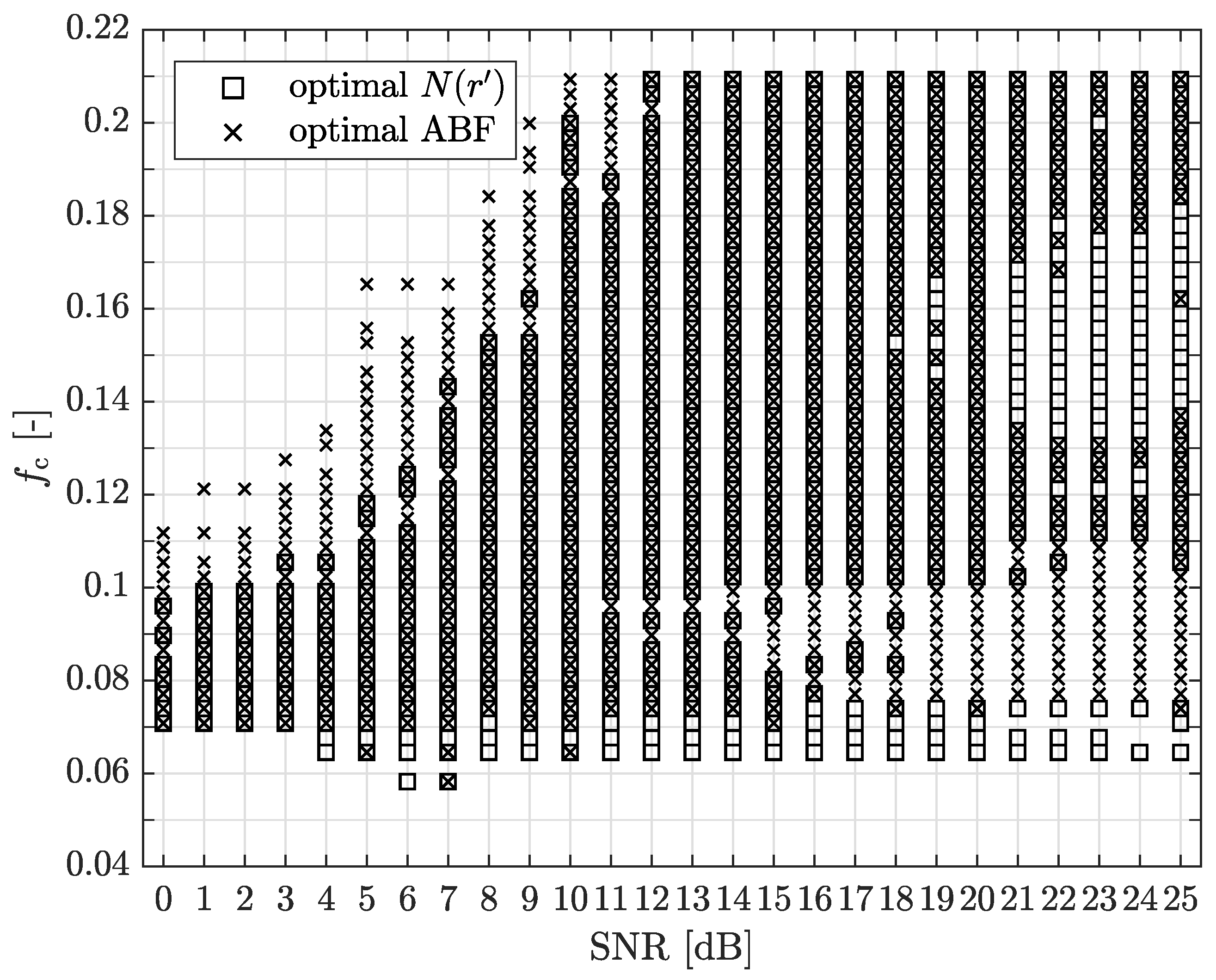
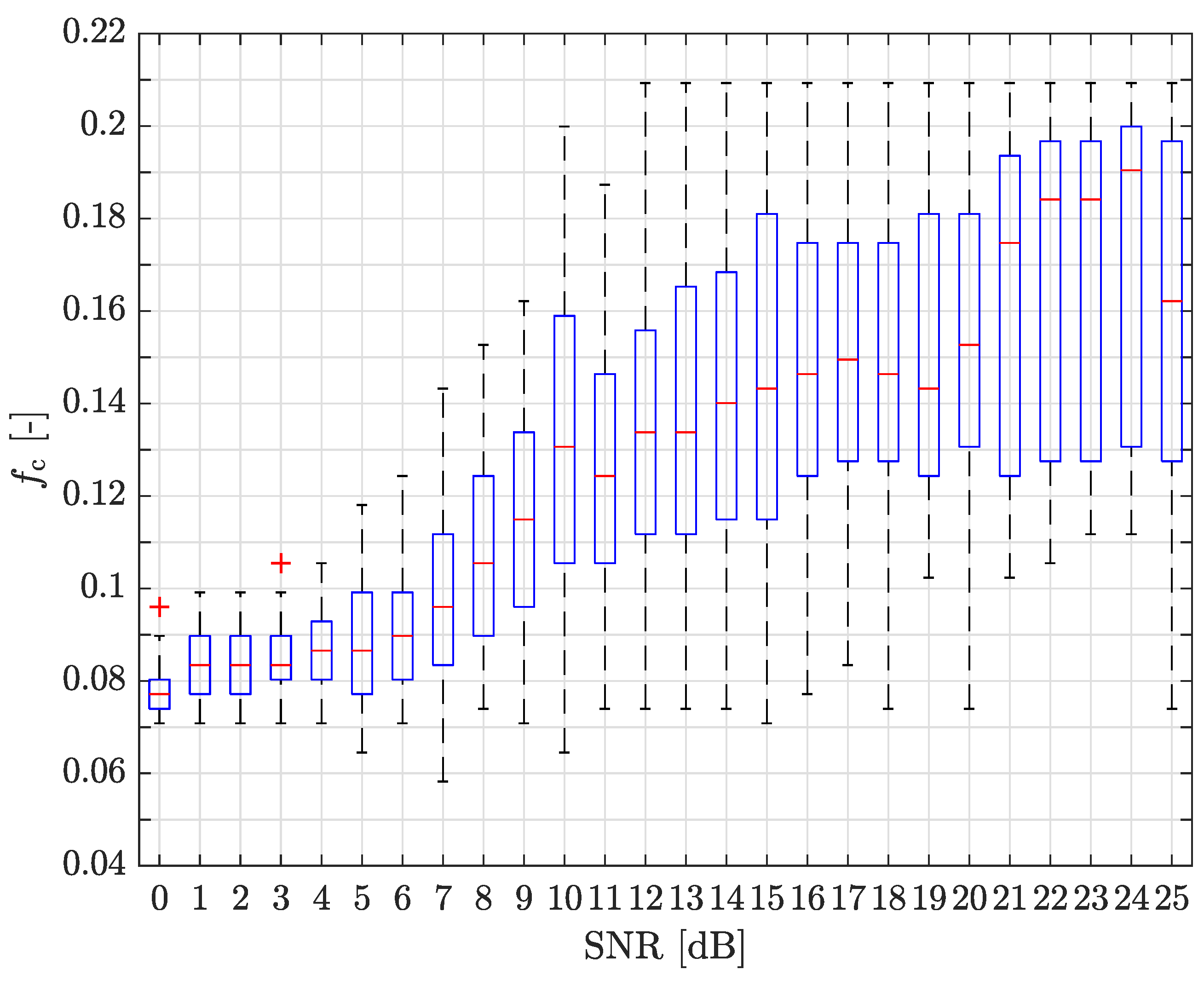
2.4. Optimal S-G Cut-Off Frequency for Application on Noisy CTF Magnitude

To determine the optimum $f_{\mathrm{c}}$, we performed 1000 Monte-Carlo simulations of the two-ray channel model with added Gaussian noise with normal distribution and zero mean to each simulated $\left|H\right(\mathrm{j}\omega \left)\right|$. The SNR varied from 0 to 25 dB with 1 dB step. The parameters of the simulation scenario are defined in Section 2.2. During the simulations, the S-G filter was used to obtain smoothed CTF for each realization of $\left|H\right(\mathrm{j}\omega \left)\right|$ at a certain SNR value. The S-G filter parameters were set to $M=200$ and varying $N=\{2,4,6,\cdots ,132\}$. According to Equation (5) we get a minimum S-G filter normalized cut-off frequency $f_{\mathrm{c},\min }=0.004721$ and a maximum S-G filter normalized cut-off frequency $f_{\mathrm{c},\max }=0.209316$. The S-G filter normalized cut-off frequency step equals 0.00314.

For each simulation loop, the estimated number of crossings $\widehat{N}\left(r^{\prime }\right)$ and $\widehat{\mathrm{ABF}}$ were compared with the corresponding nominal values $\overline{N}\left(r^{\prime }\right)=39$ and $\overline{\mathrm{ABF}}=125.1\mathrm{MHz}\pm 1\mathrm{MHz}$. The nominal values were obtained from a simulation with very high SNR (100 dB). If the estimated and nominal values were within the range ($\pm 1$), the current $f_{\mathrm{c}}$ was labeled as optimal for $N\left(r^{\prime }\right)$ or ABF and stored. Figure 2 shows these optimal values of $f_{\mathrm{c}}$ for $N\left(r^{\prime }\right)$ (marked as squares) and ABF (marked as ×) obtained by simulation of 1000 $\left|H\right(\mathrm{j}\omega \left)\right|$ realizations for each SNR value. The frequency of occurrence of individual optimal values of $f_{\mathrm{c}}$ is not considered here.

In Figure 3 we present a boxplot of the optimum $f_{\mathrm{c}}$ for individual SNR values. Only the $f_{\mathrm{c}}$ values labeled as optimal for both $N\left(r^{\prime }\right)$ and ABF were considered, together with the frequency of occurrence. In the boxplot, the median per single SNR $q_2$ is labeled as a red line within the boxplot, dashed whiskers provide information about the minimum and the maximum $f_{\mathrm{c}}$ values presented (maximum whisker length $w=1.5$) and the red plus signs denote outliers. Points are marked as outliers if they are greater than $q_3+w(q_3-q_1)$ or less than $q_1-w(q_3-q_1)$, where $q_1$ and $q_3$ are the 25-th and 75-th percentile, respectively. It is obvious that $q_2$ of the optimal $f_{\mathrm{c}}$ is expanding with increasing SNR mainly for SNR values from 6 dB to 13 dB.

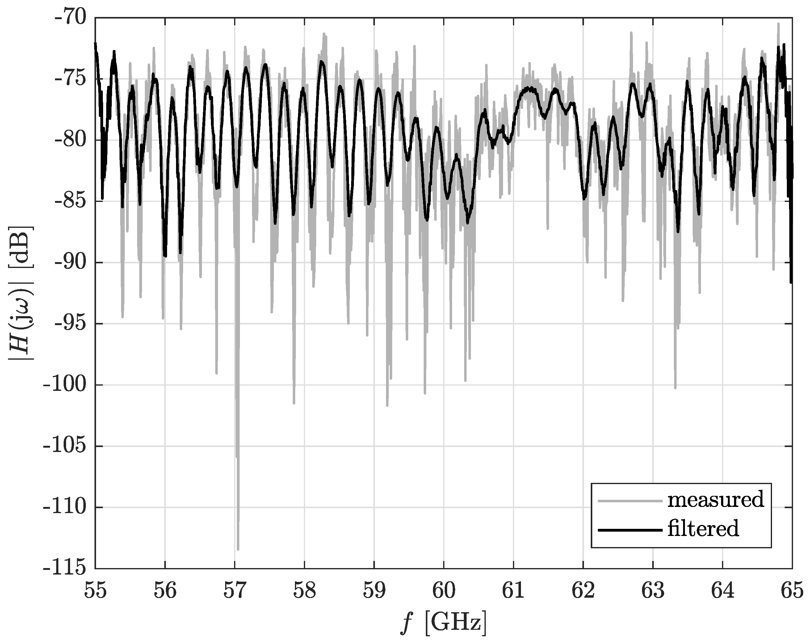
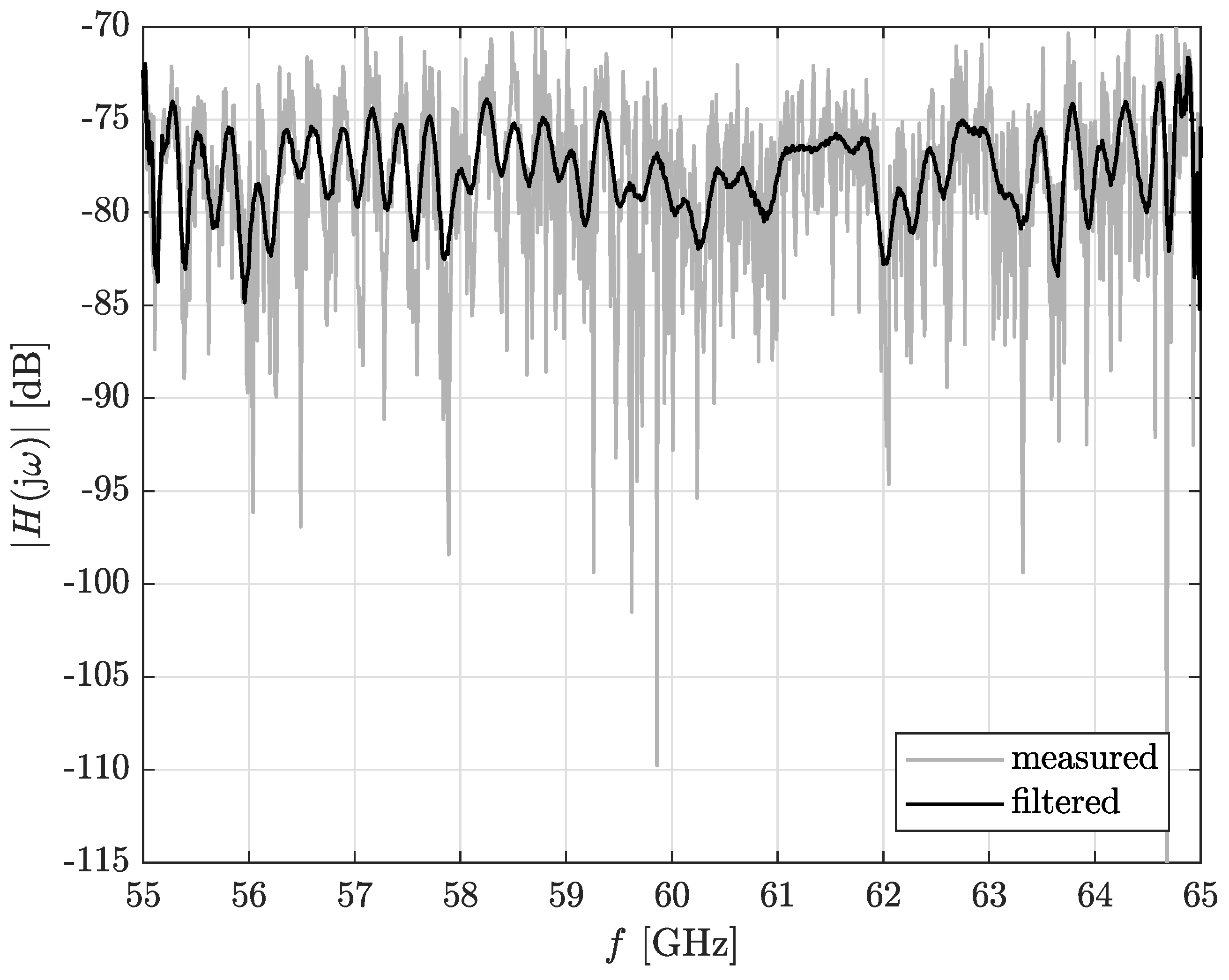
3. Application of the Savitzky–Golay Filter to the Measured CTF

In this Section, we focus on the estimation of ${\widehat{\tau }}_{\mathrm{RMS}}$ from $\left|H\right(\mathrm{j}\omega \left)\right|$ obtained by a static measurement in an anechoic chamber. Next, we test the S-G filter to reduce LCR${}_{\mathrm{f}}$ estimation error. The parameters of the measurement are listed in

Table 1. Measurement parameters. VNA = Vector Network Analyzer.

Parameter	Value
Antenna height ($h_{\mathrm{ANT}}$)	1.245 m
Antenna distance ($d_{\mathrm{ANT}}$)	2.100 m
Meas. antenna type TX	open waveguide with power amplifier
Meas. antenna type RX	open waveguide
Antenna gain ($G_{\mathrm{TX}}$)	9 dBi
TX amplifier gain ($G_{\mathrm{PA}}$)	35 dB
TX cable loss ($A_{\mathrm{c}1}$)	12 dB
RX cable loss ($A_{\mathrm{c}2}$)	26 dB
VNA intermediate frequency bandwidth ($B{W}_{\mathrm{IF}}^{\mathrm{VNA}}$)	100 Hz
Frequency range	from 55 GHz to 65 GHz
Observed bandwidth	10 GHz
Number of points in frequency domain	1001

and correspond to the scenario considered (see Section 2.2). The scheme of the measurement setup is shown in Figure 4.

The walls in the anechoic chamber were covered with absorbers, with the exception of a strip on the floor (1 m wide) between the antenna stands. At a distance of 1.05 m ($d_{\mathrm{MP}}$) from the TX antenna, a metal plate of $0.5\times 0.5$ m in size was placed and fitted. The edge of the metal plate was placed with a horizontal offset of 0.125 m over the axis of the direct path ($d_{\mathrm{ANT}}$) between the TX and RX antennas (approximately 3/4 overlapping of $d_{\mathrm{ANT}}$). If we assume only two dominant signal paths between the TX/RX antennas, then the length of the direct and reflected paths are $l_{\mathrm{LOS}}=2.1\mathrm{m}$ and $l_{\mathrm{R}}=3.26\mathrm{m}$, respectively. According to the two-ray channel model, described by Equation (1), the nominal value of the ${\overline{\tau }}_{\mathrm{RMS}}$ for the presented scenario is approximately $1.93\mathrm{ns}$ and the nominal number of crosses $\overline{N}\left(r^{\prime }\right)=39$. The correctness of ${\overline{\tau }}_{\mathrm{RMS}}$ is proven by estimation from the measured CIR with high SNR, for which ${\tau }_{\mathrm{RMS}}=1.80\mathrm{ns}\pm 0.15\mathrm{ns}$ (obtained from 10 measurements). The measurement uncertainty (Type A) is determined as $u\left(x\right)={\left((1/n(n-1)){\sum }_{k=1}^n{(x-x_{\mathrm{AM}})}^2\right)}^{1/2}$, where n is the number of observations and $x_{\mathrm{AM}}$ is the arithmetic mean of the input [17].

For the $\left|H\right(\mathrm{j}\omega \left)\right|$ measurement, the Rohde & Schwarz ZVA67 VNA was used. The VNA output power, marked $P_{\mathrm{out}}$, was swept from $-5\mathrm{dBm}$ to $-25\mathrm{dBm}$ with a step of $-5\mathrm{dB}$. The open waveguide antenna input power, including 35 dB power amplifier gain, was $18\mathrm{dBm}$ for $P_{\mathrm{out}}=-5\mathrm{dBm}$, and $-7\mathrm{dBm}$ for $P_{\mathrm{out}}=-25\mathrm{dBm}$. The free space path loss of the direct path at $f_0=60\mathrm{GHz}$ was 74.5 dB. We performed 10 measurements of $\left|H\right(\mathrm{j}\omega \left)\right|$ for each $P_{\mathrm{out}}$ value.

The measured number of the crossings $\widehat{N}\left(r^{\prime }\right)$, the MSE of ${\widehat{\tau }}_{\mathrm{RMS}}$ and $\widehat{\mathrm{ABF}}$, divided by the corresponding nominal squared value, for varying $P_{\mathrm{out}}$ are presented in

Table 2. Results of ${\widehat{\tau }}_{\mathrm{RMS}}$ and $\widehat{\mathrm{ABF}}$ estimation depending on $P_{\mathrm{out}}$. RMS = root mean square (RMS); ABF = Average Bandwidth of Fades; MSE = mean squared error.

Measured Results without Application of S-G Filter Smoothing
$P_{\mathrm{out}}$	$-5\mathrm{dBm}$	$-10\mathrm{dBm}$	$-15\mathrm{dBm}$	$-20\mathrm{dBm}$	$-25\mathrm{dBm}$
Av. $\widehat{N}\left(r^{\prime }\right)$	120.4	178.9	211.0	212.8	201.3
$\frac{{\displaystyle \mathrm{MSE}\left({\widehat{\tau }}_{\mathrm{RMS}}\right)}}{{\displaystyle {\overline{\tau }}_{\mathrm{RMS}}{}^2}}$	8.8	27.5	53.9	55.7	49.0
$u\left({\widehat{\tau }}_{\mathrm{RMS}}\right)$	±0.1 ns	±0.1 ns	±0.2 ns	±0.2 ns	±0.2 ns
$\frac{{\displaystyle \mathrm{MSE}\left(\widehat{\mathrm{ABF}}\right)}}{{\displaystyle {\overline{\mathrm{ABF}}}^2}}$	0.4	0.5	0.6	0.6	0.5
$u\left(\widehat{\mathrm{ABF}}\right)$	±1.2 MHz	±0.6 MHz	±0.4 MHz	±0.4 MHz	± 0.4 MHz
Measured Results with Application of S-G Filter Smoothing
$P_{\mathrm{out}}$	$-5\mathrm{dBm}$	$-10\mathrm{dBm}$	$-15\mathrm{dBm}$	$-20\mathrm{dBm}$	$-25\mathrm{dBm}$
Av. est. SNR	13.15 dB	9.76 dB	7.78 dB	6.92 dB	6.91 dB
Av. est. $f_{\mathrm{c}}$	0.1344	0.1280	0.1034	0.0953	0.0954
Av. $\widehat{N}\left(r^{\prime }\right)$	38.3	49.7	52.6	44.6	39.4
Av. ${\widehat{\tau }}_{\mathrm{RMS}}$	1.49 ns	1.47 ns	1.33 ns	1.44 ns	1.80 ns
$\frac{{\displaystyle \mathrm{MSE}\left({\widehat{\tau }}_{\mathrm{RMS}}\right)}}{{\displaystyle {\overline{\tau }}_{\mathrm{RMS}}{}^2}}$	0.01	0.01	0.02	0.05	0.13
$\frac{{\displaystyle \mathrm{MSE}\left(\widehat{\mathrm{ABF}}\right)}}{{\displaystyle {\overline{\mathrm{ABF}}}^2}}$	0.04	0.02	0.02	0.03	0.20

. We can see that $\widehat{N}\left(r^{\prime }\right)$ is rapidly growing with decreasing $P_{\mathrm{out}}$. The parameter $\mathrm{MSE}\left({\widehat{\tau }}_{\mathrm{RMS}}\right)/{\overline{\tau }}_{\mathrm{RMS}}{}^2$ varies from 8.8 to 55.7 and $\mathrm{MSE}\left(\widehat{\mathrm{ABF}}\right)/{\overline{\mathrm{ABF}}}^2$ varies from 0.4 to 0.6. The estimation error caused by additional crossings can be reduced by using the S-G filter. The estimation accuracy of ${\widehat{\tau }}_{\mathrm{RMS}}$ is maximized with a proper cut-off frequency $f_{\mathrm{c}}$ of the S-G filter. The proposed method was applied to the measured $\left|H\right(\mathrm{j}\omega \left)\right|$ data. To obtain SNR, the variance estimation method, developed by Garcia [18], was used. The averaged estimated value of SNR of the measured data for $P_{\mathrm{out}}=-5\mathrm{dBm}$ is $13.15\mathrm{dB}$. The estimated SNR for other $P_{\mathrm{out}}$ values (see Table 2) varied approximately from 6.91 to $9.76\mathrm{dB}$ due to distortion. The averaged optimal values of $f_{\mathrm{c}}$ at the estimated SNR varies from $0.0953$ ($P_{\mathrm{out}}=-20\mathrm{dBm}$) to $0.1344$ ($P_{\mathrm{out}}=-5\mathrm{dBm}$). For results obtained with the application of the S-G filter, the parameter $\mathrm{MSE}\left({\widehat{\tau }}_{\mathrm{RMS}}\right)/{\overline{\tau }}_{\mathrm{RMS}}{}^2$ varies from 0.01 to 0.13 and $\mathrm{MSE}\left(\widehat{\mathrm{ABF}}\right)/{\overline{\mathrm{ABF}}}^2$ varies from 0.02 to 0.20. The list of complete S-G filter parameters used for noisy $\left|H\right(\mathrm{j}\omega \left)\right|$ post-processing and the results of ${\widehat{\tau }}_{\mathrm{RMS}}$ can also be found in Table 2. The increased accuracy of ${\widehat{\tau }}_{\mathrm{RMS}}$ is evident, because averaged ${\widehat{\tau }}_{\mathrm{RMS}}$ is nearly constant and approximately equaling ${\overline{\tau }}_{\mathrm{RMS}}$ with decreasing $P_{\mathrm{out}}$. Marginal distortion is another significant advantage of using S-G filters. Examples of the noisy and filtered $\left|H\right(\mathrm{j}\omega \left)\right|$ are shown in Figure 5 and Figure 6, respectively.

4. Discussion

At the beginning of this work, we compared the basic methods for smoothing the shape of curves (to increase SNR). After the application of the smoothing methods to the data representing absolute CTF values, most of these methods subjectively distorted the shape of $\left|H\right(\mathrm{j}\omega \left)\right|$, especially in the areas of fading. It led to subsequent inaccurate estimation of the K-factor using the MLE method [15] and, thus, to inaccuracies in the ${\tau }_{\mathrm{RMS}}$ estimation. The S-G filter was selected for use in this application, mainly due to its proven smoothing and low shape distortion characteristics [12,16].

Table 3. Comparison of the application of the S-G filter and the lowpass FIR Equiripple filter on the $\left|H\right(\mathrm{j}\omega |$ segment for $P_{\mathrm{out}}=-5\mathrm{dBm}$ and $-10\mathrm{dBm}$ (frequency from 55 GHz to 56 GHz).

S-G Filter		Lowpass FIR Filter (Equiripple)
	$P_{\mathrm{out}}$ = $-5\mathrm{dBm}$ $f_{\mathrm{c}}$ = $0.1145$ $P_0$ = $-78.2\mathrm{dB}$ $\widehat{N}\left(r^{\prime }\right)$ = 31 ${\widehat{\tau }}_{\mathrm{RMS}}$ = $1.48\mathrm{ns}$ $\widehat{\mathrm{ABF}}$ = $177.7\mathrm{MHz}$		$P_{\mathrm{out}}$ = $-5\mathrm{dBm}$ $f_{\mathrm{c}}$ = $0.11$ $P_0$ = $-79.3\mathrm{dB}$ $\widehat{N}\left(r^{\prime }\right)$ = 29 ${\widehat{\tau }}_{\mathrm{RMS}}$ = $1.63\mathrm{ns}$ $\widehat{\mathrm{ABF}}$ = $199.8\mathrm{MHz}$
	$P_{\mathrm{out}}$ = $-10\mathrm{dBm}$ $f_{\mathrm{c}}$ = $0.0771$ $P_0$ = $-77.3\mathrm{dB}$ $\widehat{N}\left(r^{\prime }\right)$ = 29 ${\widehat{\tau }}_{\mathrm{RMS}}$ = $0.97\mathrm{ns}$ $\widehat{\mathrm{ABF}}$ = $191.5\mathrm{MHz}$		$P_{\mathrm{out}}$ = $-10\mathrm{dBm}$ $f_{\mathrm{c}}$ = $0.08$ $P_0$ = $-79.3\mathrm{dB}$ $\widehat{N}\left(r^{\prime }\right)$ = 62 ${\widehat{\tau }}_{\mathrm{RMS}}$ = $2.97\mathrm{ns}$ $\widehat{\mathrm{ABF}}$ = $90.3\mathrm{MHz}$

compares the results of applying the S-G (left column) filter and the lowpass FIR (right column) filter (Equiripple) to the same $\left|H\right(\mathrm{j}\omega \left)\right|$ segment for $P_{\mathrm{out}}=-5\mathrm{dBm}$ and $-10\mathrm{dBm}$. The lowpass FIR filter order is equal to the S-G filter order, and the cut-off frequencies are approximately the same. Note that the results shown in this table refer to the entire measured frequency band (from 55 to 65 GHz). The results for $P_{\mathrm{out}}=-5\mathrm{dBm}$ are similar for both filters and correspond to the expected CTF values with a high SNR. By contrast, for $P_{\mathrm{out}}=-10\mathrm{dBm}$, the results obtained by applying the lowpass FIR filter already show a greater deviation from the expected value. Some distortion of the $\left|H\right(\mathrm{j}\omega \left)\right|$ curve shape could be observed, as well. As mentioned above, the S-G filter was used and tested in this application. However, it cannot be generally claimed that this is the only general solution to this issue. Comparison with other smoothing methods would bring further useful insights into this issue.

The two-ray channel model serves as a means of modeling the definite number of $\left|H\right(\mathrm{j}\omega \left)\right|$ crossings through the level $P_0$ (3). It also serves to obtain an approximate estimate of the range of suitable S-G filter cut-off frequencies $f_{\mathrm{c}}$ for application to noisy $\left|H\right(\mathrm{j}\omega \left)\right|$ and illustrate whether it adds some improvement to the basic ${\tau }_{\mathrm{RMS}}$ estimation method described by Witrisal [2]. If we relate the used two-ray channel model to the current widely utilized and discussed two-wave channel model with diffuse power fading (TWDP), which assumess an interference of two strong signals (specular components) and a number of diffuse signals, then the ratio of specular-to-diffuse power $K_{\mathrm{TWDP}}\to \infty$ (only specular components are considered) and the ratio of the specular components ${\Delta }_{\mathrm{TWDP}}$ equals 1 [13]. The examination of a number of combinations of the channel model parameters and the channel model types goes beyond the scope of this work.

5. Conclusions

In this paper, we presented a novel, simple and easy to use method to increase the accuracy of the RMS channel delay spread estimation from scalar power measurement in frequency domain. We described the utilization of the S-G filtering method as a complement to the level crossing rate ${\tau }_{\mathrm{RMS}}$ estimation method in the frequency domain. For a correct S-G smoothing process, a set of optimal $f_{\mathrm{c}}$ frequencies were obtained by the Monte-Carlo simulation of a two-ray channel model. The usability of the S-G smoothing method is illustrated by its application on the CTF in mmWave bands, measured in an anechoic chamber at various signal power dynamics. It was proven that using the S-G filter brings a noticeable increase in the ${\tau }_{\mathrm{RMS}}$ estimation accuracy with minimal shape distortion. Future work could be focused on defining an adaptive algorithm to find an optimal S-G filter settings for this purpose.

References

1. Molisch, A.F. Statistical properties of the RMS delay-spread of mobile radio channels with independent Rayleigh fading paths. IEEE Trans. Veh. Technol. 1996, 45, 201–204. [Google Scholar] [CrossRef]
2. Witrisal, K. On estimating the RMS delay spread from the frequency-domain level crossing rate. IEEE Commun. Lett. 2001, 5, 287–289. [Google Scholar] [CrossRef] [Green Version]
3. Chandra, A.; Prokes, A.; Mikulasek, T.; Blumenstein, J.; Kukolev, P.; Zemen, T.; Mecklenbrauker, C.F. Frequency-domain in-vehicle UWB channel modeling. IEEE Trans. Veh. Technol. 2016, 65, 3929–3940. [Google Scholar] [CrossRef]
4. Muquet, B.; Wang, Z.; Giannakis, G.B.; De Courville, M.; Duhamel, P. Cyclic prefix or zero padding for wireless multicarrier transmissions? IEEE Trans. Commun. 2002, 50, 2136–2148. [Google Scholar] [CrossRef] [Green Version]
5. Molisch, A.F. Wireless Communications, 2nd ed.; John Wiley and Sons: Chichester, UK, 2011. [Google Scholar]
6. Flikkema, P.G.; Johnson, S.G. A comparison of time- and frequency-domain wireless channel sounding techniques. In Proceedings of the SOUTHEASTCON’96, Tampa, FL, USA, 11–14 April 1996; pp. 488–491. [Google Scholar]
7. Witrisal, K.; Kim, Y.-H.; Prasad, R. RMS delay spread estimation technique using non-coherent channel measurements. Electron. Lett. 1998, 34, 1918–1919. [Google Scholar] [CrossRef]
8. Witrisal, K.; Bohdanowicz, A. Influence of noise on a novel RMS delay spread estimation method. In Proceedings of the 11th IEEE International Symposium on Personal Indoor and Mobile Radio Communications PIMRC, London, UK, 18–21 September 2000; pp. 560–566. [Google Scholar]
9. Bohdanowicz, A.; Janssen, G.J.M.; Pietrzyk, S. Wideband indoor and outdoor multipath channel measurements at 17 GHz. In Proceedings of the IEEE VTS 50th Vehicular Technology Conference (VTC 1999-Fall), Amsterdam, The Netherlands, 19–22 September 1999; pp. 1998–2003. [Google Scholar]
10. Prokes, A.; Mikulasek, T.; Blumenstein, J.; Vychodil, J. Usability of Hilbert transform for complex channel transfer function calculation in 60 GHz band. In Proceedings of the Progress in Electromagnetics Research Symposium—Fall (PIERS-FALL), Singapore, 19–22 November 2017; pp. 2945–2951. [Google Scholar]
11. Savitzky, A.; Golay, M.J.E. Smoothing and differentation of data by simplified least squares procedures. Analy. Chem. 1964, 36, 1627–1639. [Google Scholar] [CrossRef]
12. Krishnan, S.R.; Seelamantula, C.S. On the selection of optimum Savitzky-Golay filters. IEEE Trans. Signal Process. 2013, 61, 380–391. [Google Scholar] [CrossRef]
13. Zöchmann, E.; Hofer, M.; Lerch, M.; Pratschner, S.; Bernado, L.; Blumenstein, J.; Prokes, A. Position-specific statistics of 60 GHz vehicular channels during overtaking. IEEE Access 2019, 7, 14216–14232. [Google Scholar] [CrossRef]
14. Zöchmann, E.; Guan, K.; Rupp, M. Two-ray models in mmWave communications. In Proceedings of the IEEE 18th International Workshop on Signal Processing Advances in Wireless Communications (SPAWC), Sapporo, Japan, 3–6 July 2017; pp. 1–5. [Google Scholar]
15. Chen, Y.; Beaulieu, N.C. Maximum likelihood estimation of the K factor in Ricean fading channels. IEEE Commun. Lett. 2005, 9, 1040–1042. [Google Scholar] [CrossRef]
16. Schafer, R.W. What is Savitzky-Golay filter? IEEE Signal Proc. Mag. 2011, 28, 111–117. [Google Scholar] [CrossRef]
17. Evaluating Uncertainty Components: Type A. The NIST Reference on Constants, Units, and Uncertainity. Available online: https://physics.nist.gov/cuu/Uncertainty/typea.html (accessed on 2 November 2019).
18. Garcia, D. Robust smoothing of gridded data in one and higher dimensions with missing values. Comp. Stat. Data Anal. 2010, 54, 1167–1178. [Google Scholar] [CrossRef] [PubMed] [Green Version]
Figure 1. Influence of Additive White Gaussian Noise (AWGN) on three main parts of the τ RMS estimation process (a): N ( r ) , K, P 0 , and on the corresponding resultant τ RMS and Average Bandwidth of Fades (ABF) estimated parameters (b). Two-ray channel model ( d ANT = 2.1 m , h ANT = 1.245 m , f min = 55 GHz , f max = 65 GHz ).
Electronics 08 01530 g001
Figure 2. Optimal normalized cut-off frequencies of the Savitzky-Golay (S-G) filter, obtained by simulation, for a two-ray channel model based on the presented scenario ( d ANT = 2.1 m , h ANT = 1.245 m , f min = 55 GHz , f max = 65 GHz ) depending on Signal-to-Noise Ratio (SNR).
Electronics 08 01530 g002
Figure 3. The boxplot of the optimal normalized cut-off frequencies of the S-G filter, obtained by simulation, for a two-ray channel model based on the presented scenario ( d ANT = 2.1 m , h ANT = 1.245 m , f min = 55 GHz , f max = 65 GHz ) depending on SNR.
Electronics 08 01530 g003
Figure 4. The measurement setup scheme (in anechoic chamber).
Electronics 08 01530 g004
Figure 5. Example of measured and filtered | H ( j ω ) | ( P out = 5 dBm , estimated SNR = 13.64 dB and S-G filter f c = 0.1145 ). Measurement scenario: d ANT = 2.1 m , h ANT = 1.245 m , f min = 55 GHz , f max = 65 GHz .
Electronics 08 01530 g005
Figure 6. Example of measured and filtered | H ( j ω ) | ( P out = 10 dBm , estimated SNR = 9.77 dB and S-G filter f c = 0.0771 ). Measurement scenario: d ANT = 2.1 m , h ANT = 1.245 m , f min = 55 GHz , f max = 65 GHz .
Electronics 08 01530 g006