Design and Analysis of Refined Inspection of Field Conditions of Oilfield Pumping Wells Based on Rotorcraft UAV Technology


Abstract
1. Introduction
2. Related Works
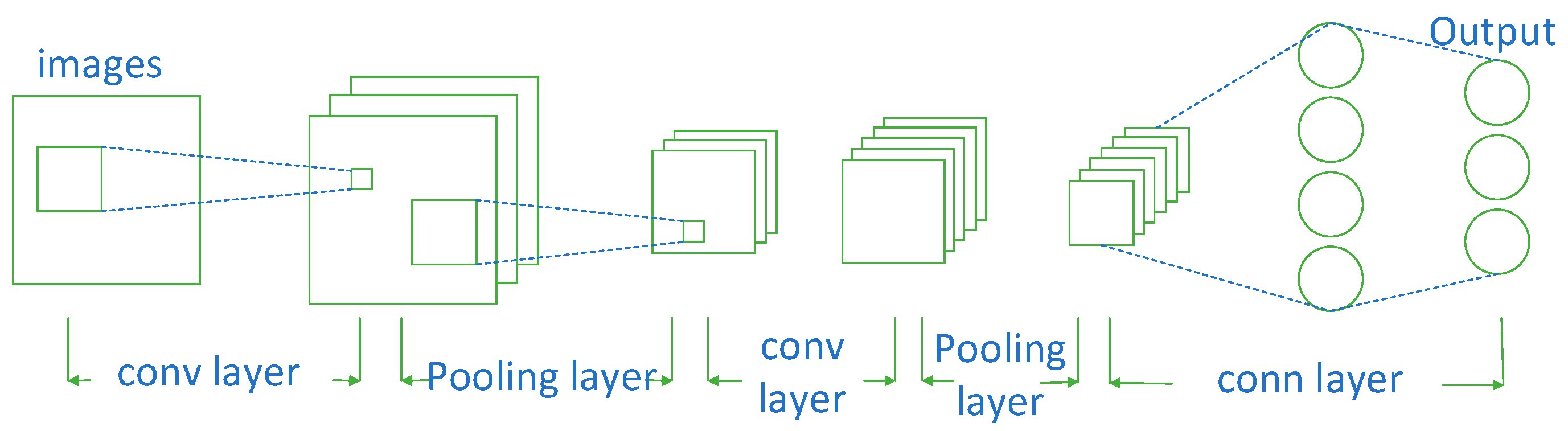
2.1. The Basics of Convolutional Neural Networks (CNNs)
2.2. Object Detection
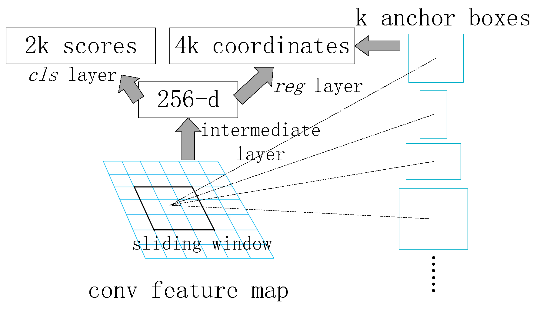
2.2.1. Faster R-CNN
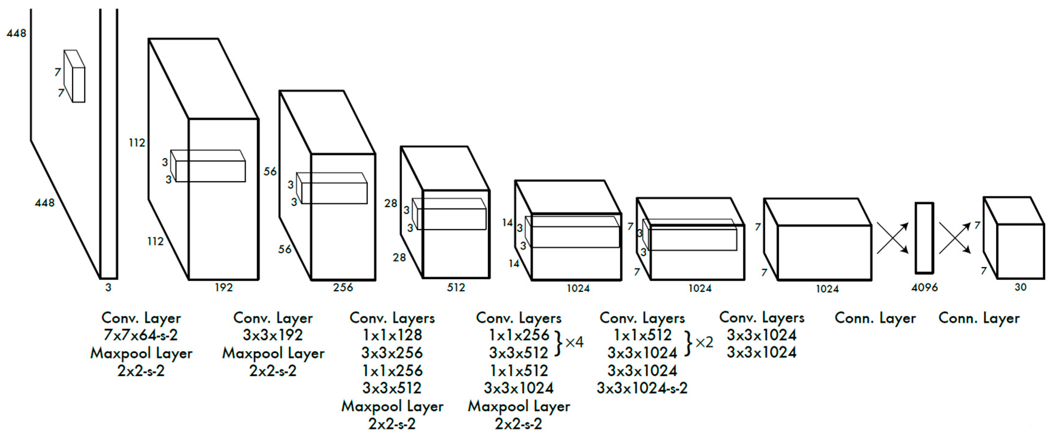
2.2.2. YOLO
2.2.3. SSD
- Multi-scale feature graph is adopted for detection—pyramid feature.
- Set Default boxes.
- Determination of Default boxes size.
- Convolution was used for detection.
3. Using the YLTS Framework to Realize the Pumping Unit Working Condition Detection of the Aerial Image of the UAV
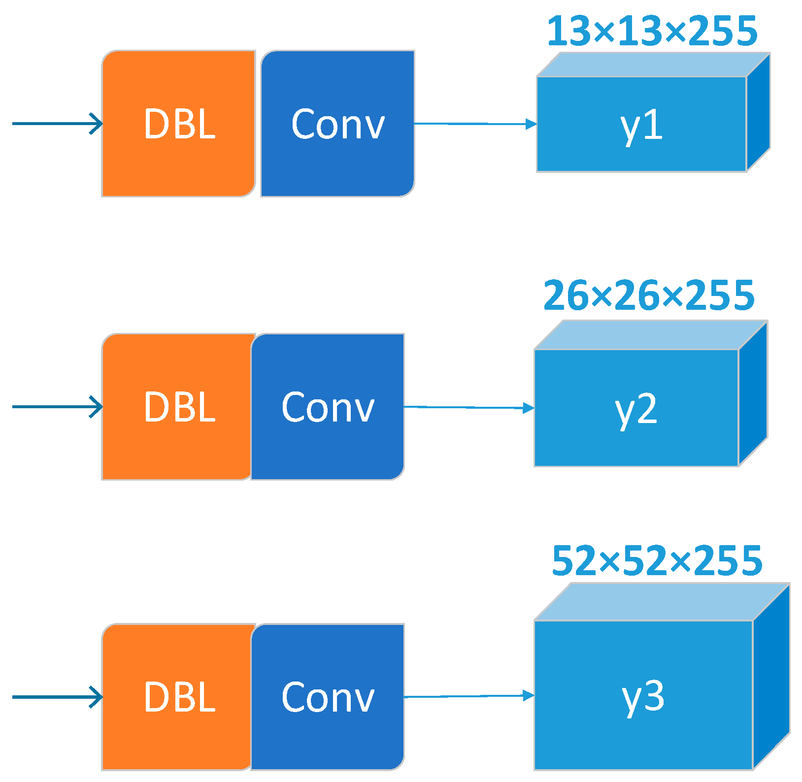
3.1. Using YOLOv3 as a Detector of the YLTS Framework to Detect the Pumping Unit and the Head Working
3.2. Use the Sort Algorithm as a Tracker of the YLTS Framework to Track the Pumping Unit and the Head Working
- When the first frame comes in, the detected target is initialized and a new tracker is created, labeled with an id.
- When the following frame comes in, the state prediction and covariance prediction generated by the previous frame detection box are obtained first in the Kalman filter. The target state prediction and the IOU of the frame detection box are respectively obtained, the maximum matching of the IOU is obtained by the Hungarian assignment algorithm, and the matching pair in which the matching value is smaller than the IOU threshold is removed.
- The Kalman tracker is updated using the matched target detection frame in this frame to calculate the Kalman gain, status update, and covariance update. The status update value is output as the tracking frame of this frame. The tracker for targets that are not matched in this frame are reinitialized [35,36].
4. Experiment and Analysis
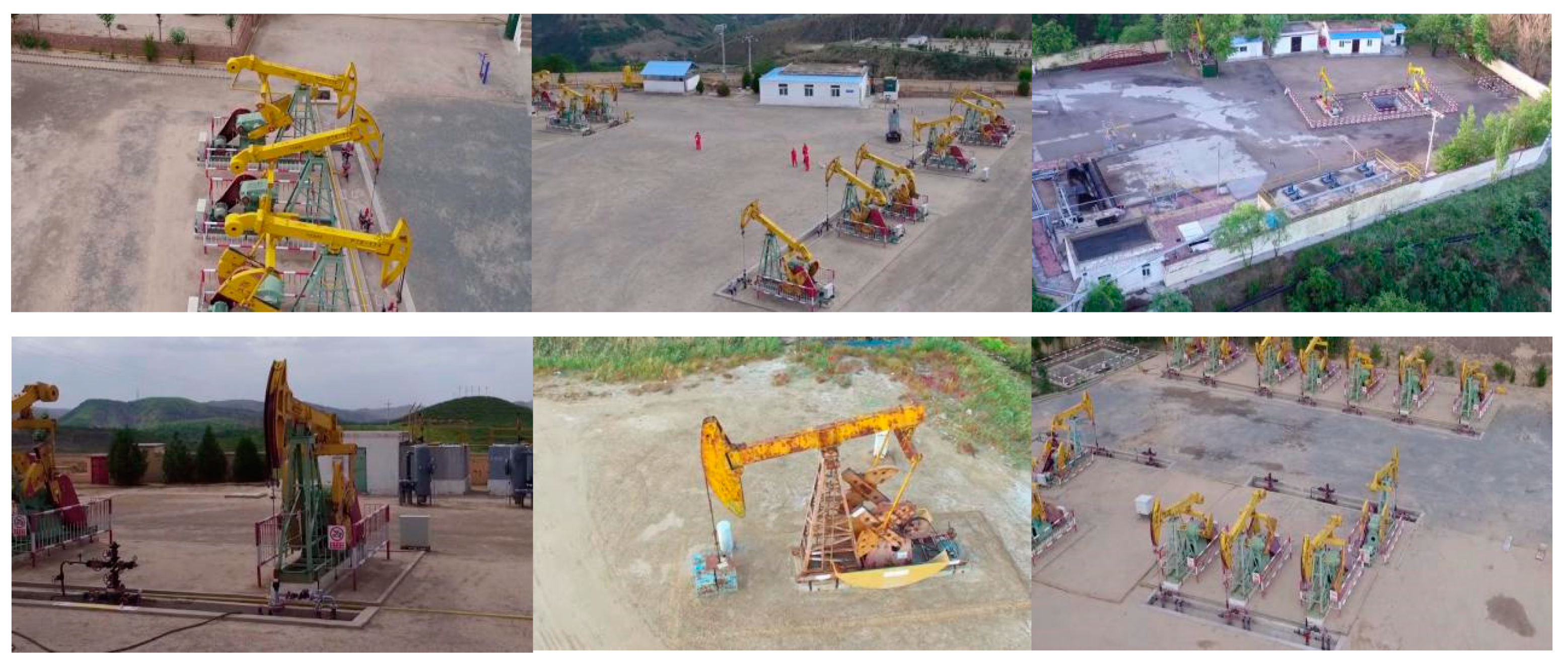
4.1. Description of the Training Data
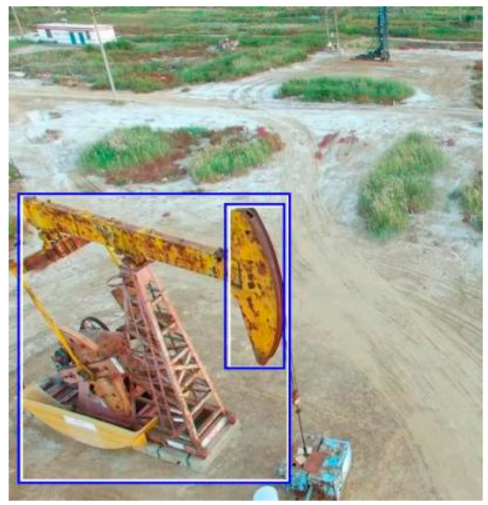
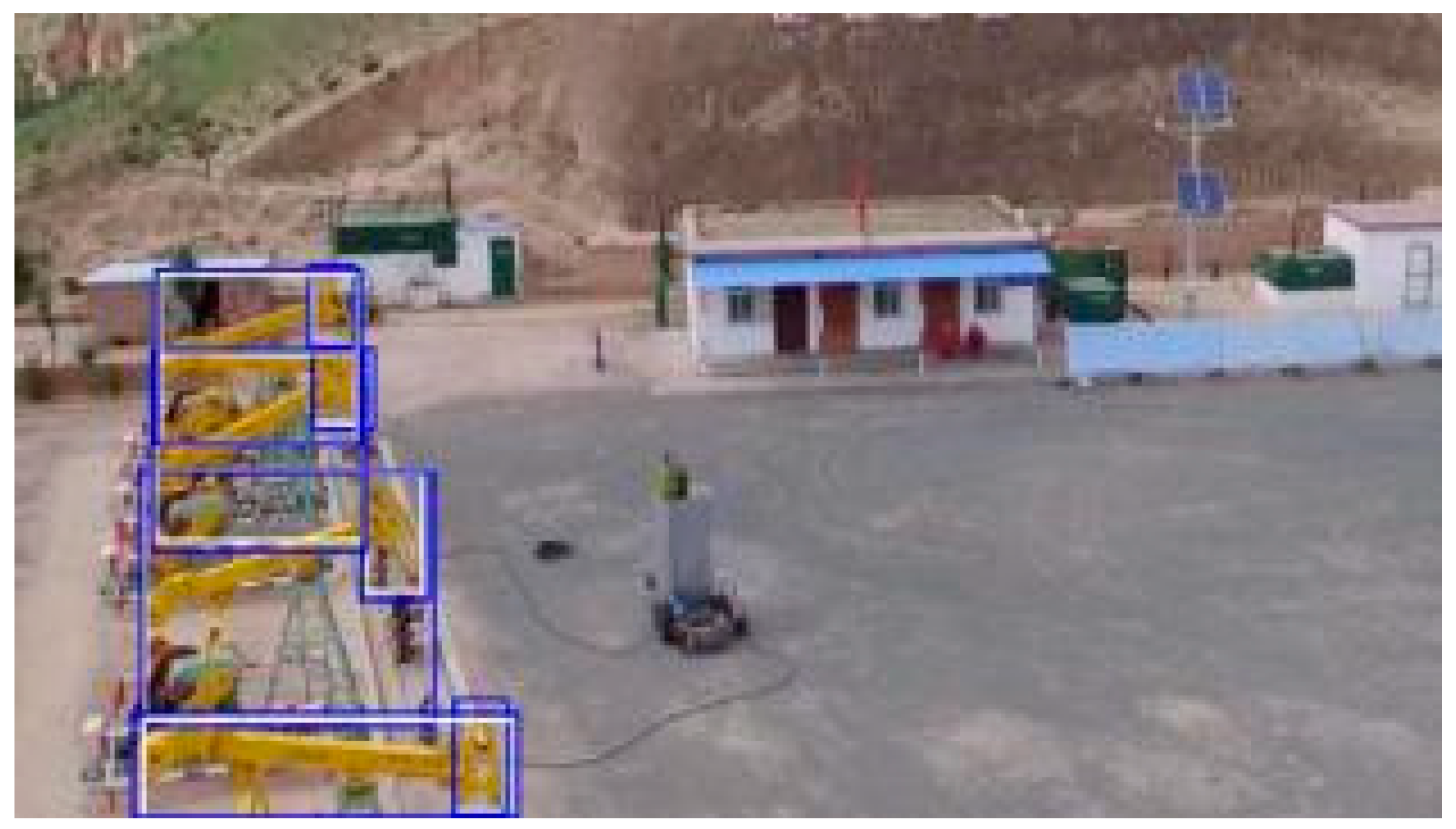
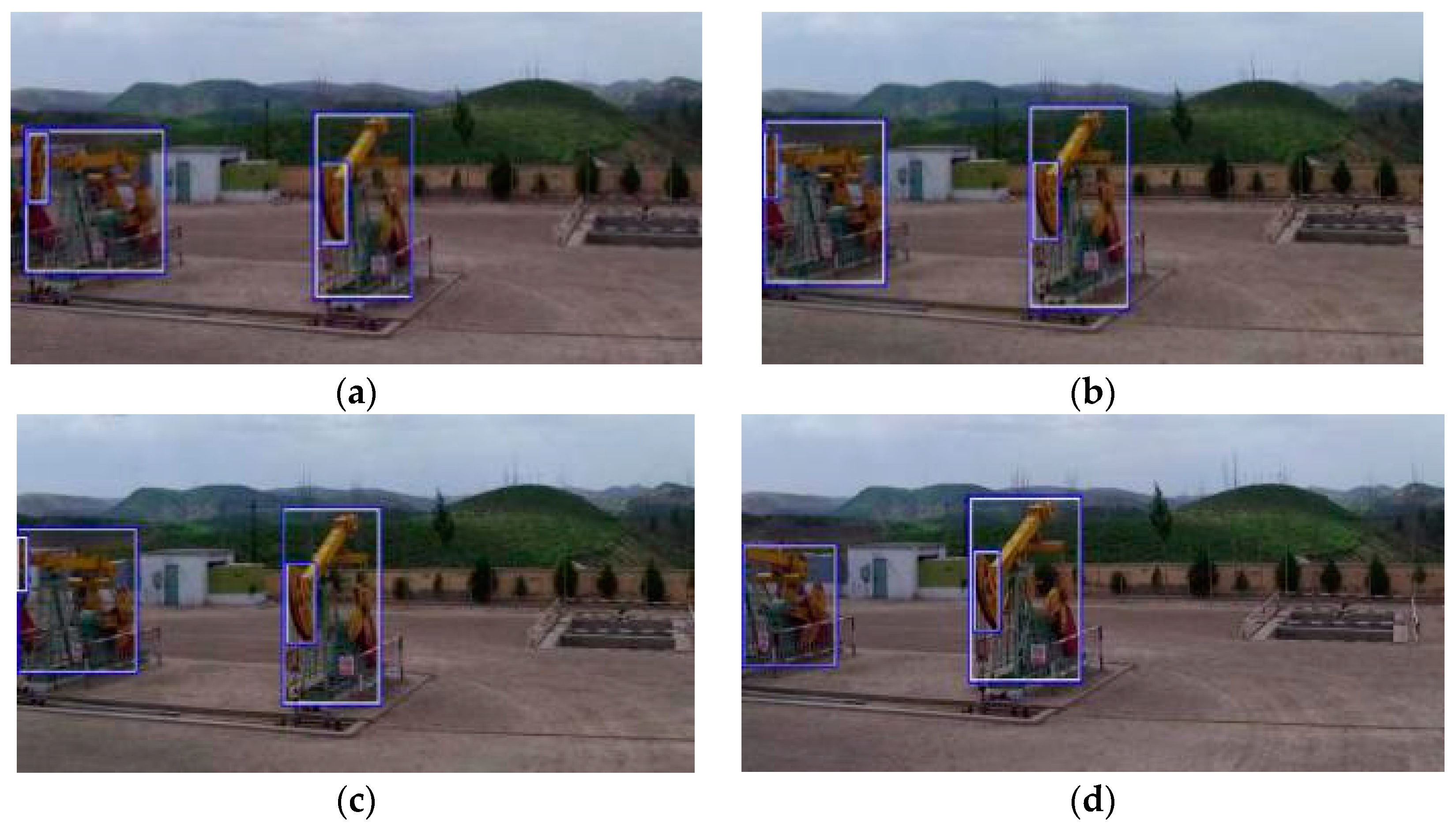
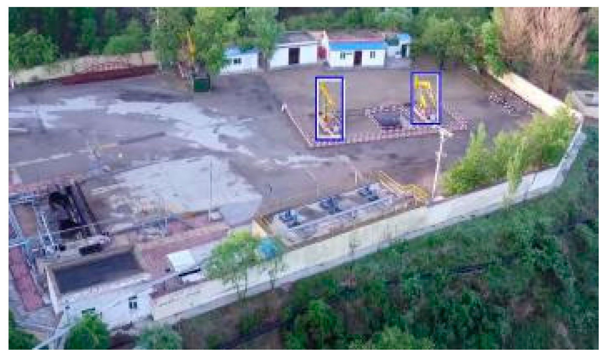
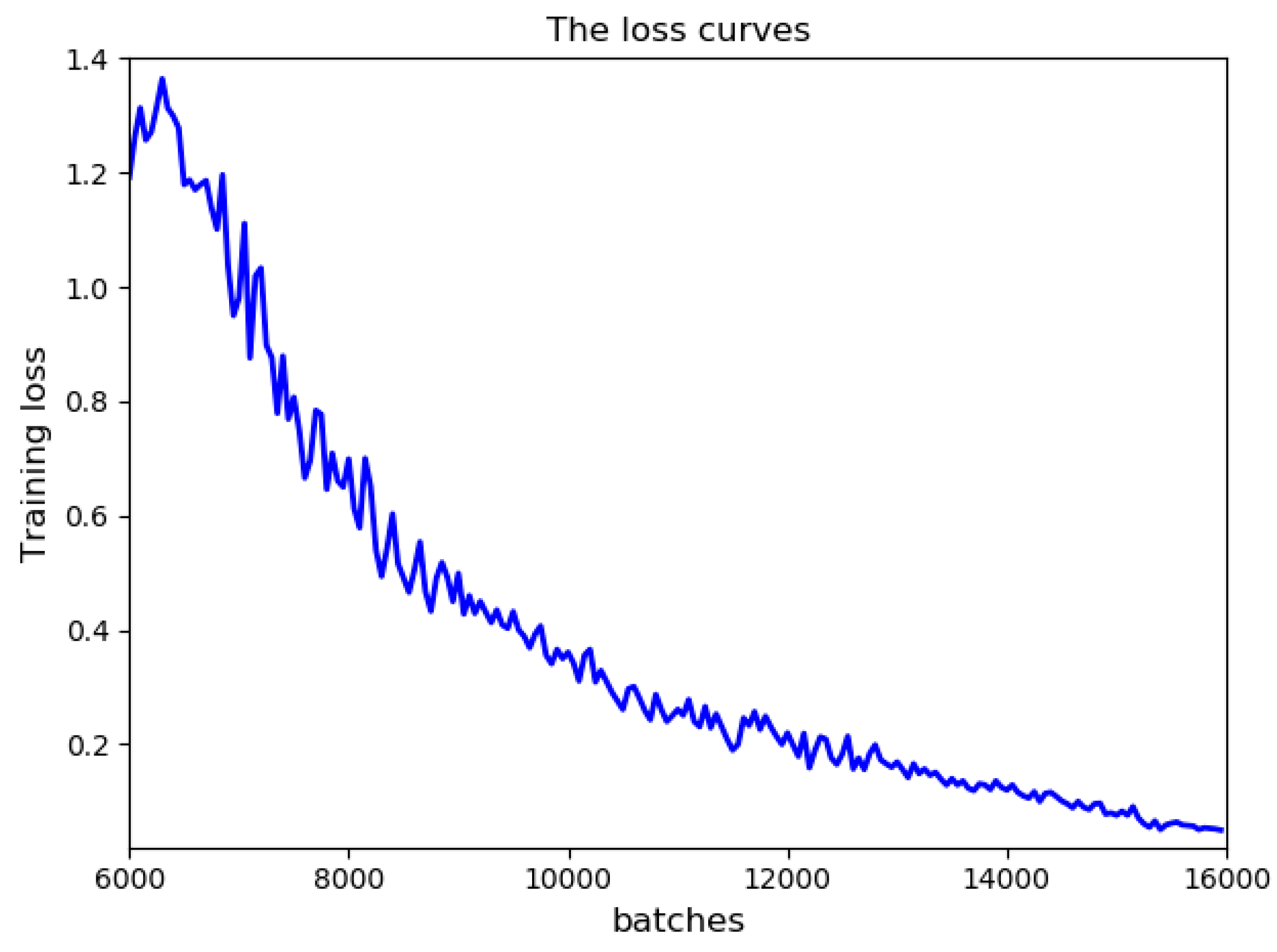
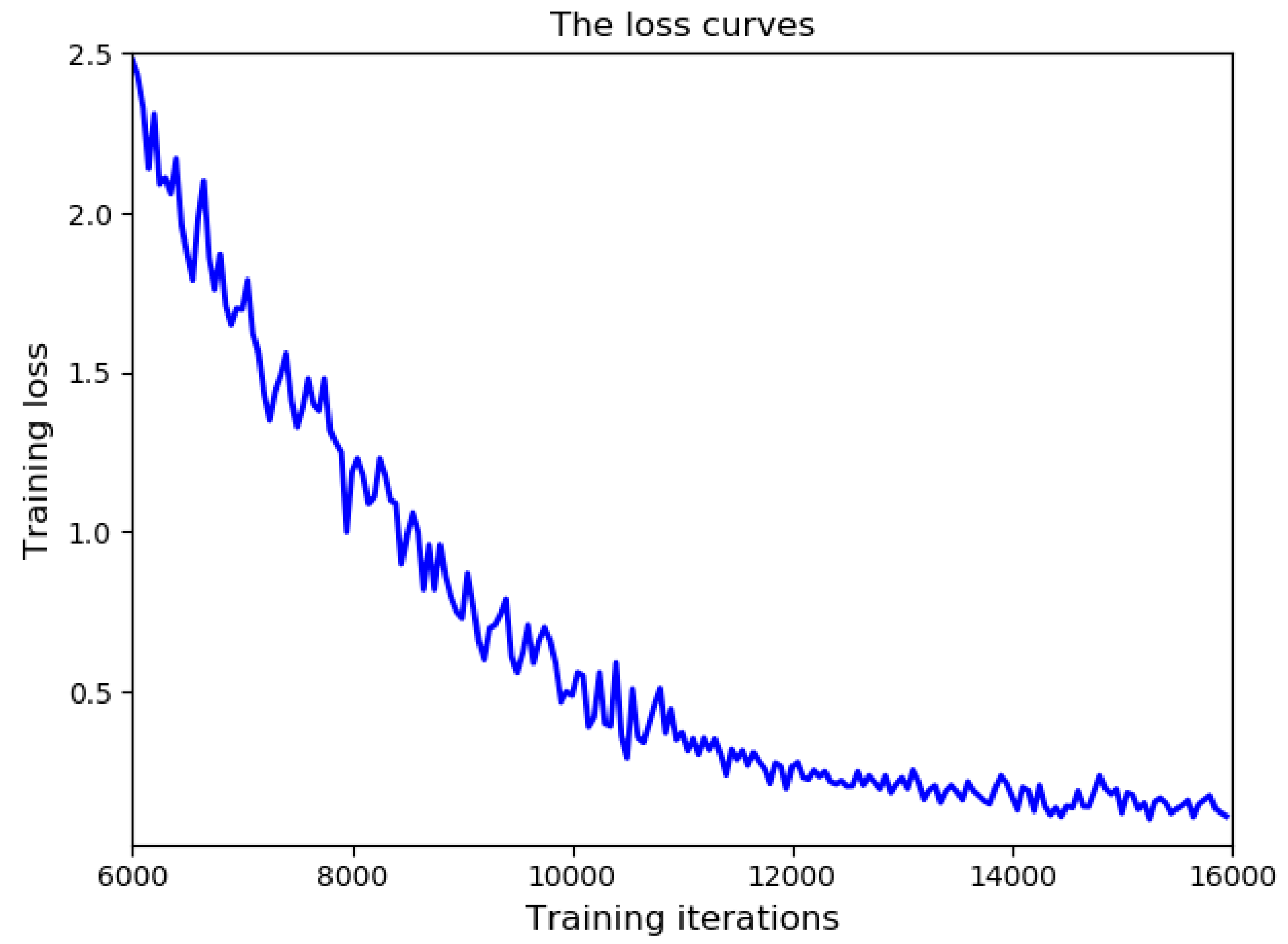
4.2. Experimental Results and Comparison
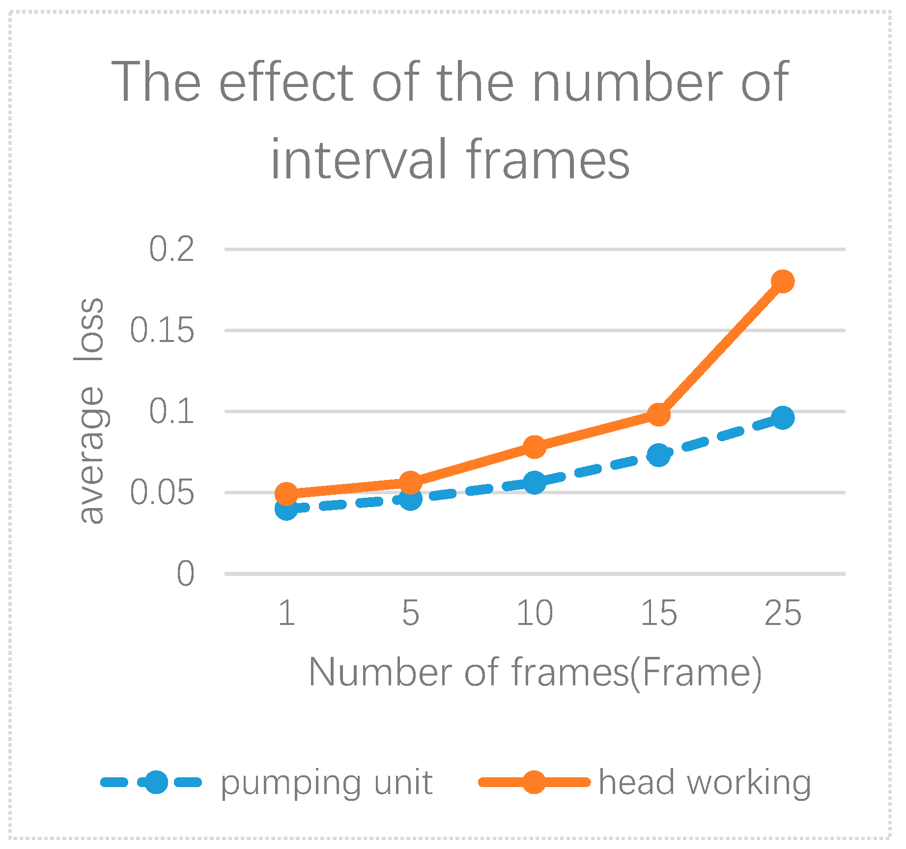
4.3. The Analysis of Experiment
5. Conclusions and Future Works
Author Contributions
Funding
Acknowledgments
Conflicts of Interest
References
- Chen, H.; Wu, C.; Huang, W.; Wu, Y.; Xiong, N. Design and Application of System with Dual-Control of Water and Electricity Based on Wireless Sensor Network and Video Recognition Technology. Int. J. Distrib. Sens. Netw. 2018, 14, 1550147718795951. [Google Scholar] [CrossRef]
- Li, X.; Zhou, C.; Tian, Y.-C.; Xiong, N.; Qin, Y. Asset-Based Dynamic Impact Assessment of Cyberattacks for Risk Analysis in Industrial Control Systems. IEEE Trans. Ind. Inform. 2018, 14, 608–618. [Google Scholar] [CrossRef]
- Ju, C.; Son, H. Multiple Uav Systems for Agricultural Applications: Control, Implementation, and Evaluation. Electronics 2018, 7, 162. [Google Scholar] [CrossRef]
- Hu, G.; Yang, Z.; Han, J.; Huang, L.; Gong, J.; Xiong, N. Aircraft Detection in Remote Sensing Images Based on Saliency and Convolution Neural Network. EURASIP J. Wirel. Comm. Netw. 2018, 2018, 26. [Google Scholar] [CrossRef]
- Hua, X.; Wang, X.; Rui, T.; Wang, D.; Shao, F. Real-Time Object Detection in Remote Sensing Images Based on Visual Perception and Memory Reasoning. Electronics 2019, 8, 1151. [Google Scholar] [CrossRef]
- Aksu, D.; Aydin, M.A. Detecting Port Scan Attempts with Comparative Analysis of Deep Learning and Support Vector Machine Algorithms. In Proceedings of the 2018 International Congress on Big Data, Deep Learning and Fighting Cyber Terrorism (IBIGDELFT), Ankara, Turkey, 3–4 December 2018. [Google Scholar] [CrossRef]
- Wu, C.; Luo, C.; Xiong, N.; Zhang, W.; Kim, T. A Greedy Deep Learning Method for Medical Disease Analysis. IEEE Access 2018, 6, 20021–20030. [Google Scholar] [CrossRef]
- Huang, H.; Xu, Y.; Huang, Y.; Yang, Q.; Zhou, Z. Pedestrian Tracking by Learning Deep Features. J. Vis. Commun. Image Represent. 2018, 57, 172–175. [Google Scholar] [CrossRef]
- Wang, S.; Wu, C.; Gao, L.; Yao, Y. Research on Consistency Maintenance of the Real-Time Image Editing System Based on Bitmap. In Proceedings of the 2014 IEEE 18th International Conference on Computer Supported Cooperative Work in Design (CSCWD), Hsinchu, Taiwan, 21–23 May 2014. [Google Scholar] [CrossRef]
- Zhao, J.; Xu, H.; Liu, H.; Wu, J.; Zheng, Y.; Wu, D. Detection and Tracking of Pedestrians and Vehicles Using Roadside Lidar Sensors. Transp. Res. Part C Emerg. Technol. 2019, 100, 68–87. [Google Scholar] [CrossRef]
- Jiang, X.; Fang, Z.; Xiong, N.N.; Gao, Y.; Huang, B.; Zhang, J.; Yu, L.; Harrington, P. Data Fusion-Based Multi-Object Tracking for Unconstrained Visual Sensor Networks. IEEE Access 2018, 6, 13716–13728. [Google Scholar] [CrossRef]
- Liu, C.; Zhou, A.; Wu, C.; Zhang, G. Image Segmentation Framework Based on Multiple Feature Spaces. IET Image Process. 2015, 9, 271–279. [Google Scholar] [CrossRef]
- Yang, J.C.; Jiao, Y.; Xiong, N.; Park, D.S. Fast Face Gender Recognition by Using Local Ternary Pattern and Extreme Learning Machine. TIIS 2013, 7, 1705–1720. [Google Scholar]
- Xue, W.; Wenxia, X.; Guodong, L. Image Edge Detection Algorithm Research Based on the Cnns Neighborhood Radius Equals 2. In Proceedings of the 2016 International Conference on Smart Grid and Electrical Automation (ICSGEA), Zhangjiajie, China, 11–12 August 2016. [Google Scholar] [CrossRef]
- Lecun, Y.; Bottou, L.; Bengio, Y.; Haffner, P. Gradient-Based Learning Applied to Document Recognition. Proc. IEEE 1998, 86, 2278–2324. [Google Scholar] [CrossRef]
- Wan, L.D.; Zeiler, M.; Zhang, S.; Lecun, Y.; Fergus, R. Regularization of Neural Networks Using Dropconnect. Int. Conf. Mach. Learn. 2013, 28, 1058–1066. [Google Scholar]
- Wang, Z.; Lu, W.; He, Y.; Xiong, N.; Wei, J. Re-Cnn: A Robust Convolutional Neural Networks for Image Recognition; Springer: Berlin, Germany, 2018. [Google Scholar]
- Napiorkowska, M.; Petit, D.; Marti, P. Three Applications of Deep Learning Algorithms for Object Detection in Satellite Imagery. In Proceedings of the IGARSS 2018-2018 IEEE International Geoscience and Remote Sensing Symposium, Valencia, Spain, 22–27 July 2018. [Google Scholar] [CrossRef]
- Ren, S.; He, K.; Girshick, R.; Sun, J. Faster R-Cnn: Towards Real-Time Object Detection with Region Proposal Networks. IEEE Trans. Pattern Anal. Mach. Intell. 2017, 39, 1137–1149. [Google Scholar] [CrossRef]
- Lan, W.; Dang, J.; Wang, Y.; Wang, S. Pedestrian Detection Based on Yolo Network Model. In Proceedings of the 2018 IEEE International Conference on Mechatronics and Automation (ICMA), Changchun, China, 5–8 August 2018. [Google Scholar] [CrossRef]
- Wang, X.; Hua, X.; Xiao, F.; Li, Y.; Hu, X.; Sun, P. Multi-Object Detection in Traffic Scenes Based on Improved Ssd. Electronics 2018, 7, 302. [Google Scholar] [CrossRef]
- Biswas, D.; Su, H.; Wang, C.; Stevanovic, A.; Wang, W. An Automatic Traffic Density Estimation Using Single Shot Detection (Ssd) and Mobilenet-Ssd. Phys. Chem. Earth Parts A/B/C 2018, 110, 176–184. [Google Scholar] [CrossRef]
- Kitayama, T.; Lu, H.; Li, Y.; Kim, H. Detection of Grasping Position from Video Images Based on Ssd. In Proceedings of the 2018 18th International Conference on Control, Automation and Systems (ICCAS), Daegwallyeong, Korea, 17–20 October 2018. [Google Scholar]
- Zhang, H.; Gao, L.; Xu, M.; Wang, Y. An Improved Probability Hypothesis Density Filter for Multi-Target Tracking. Optik 2019, 182, 23–31. [Google Scholar] [CrossRef]
- Yang, T.; Cappelle, C.; Ruichek, Y.; El Bagdouri, M. Online Multi-Object Tracking Combining Optical Flow and Compressive Tracking in Markov Decision Process. J. Vis. Commun. Image Represent. 2019, 58, 178–186. [Google Scholar] [CrossRef]
- Shinde, S.; Kothari, A.; Gupta, V. Yolo Based Human Action Recognition and Localization. Proced. Comput. Sci. 2018, 133, 831–838. [Google Scholar] [CrossRef]
- Krawczyk, Z.; Starzyński, J. Bones Detection in the Pelvic Area on the Basis of Yolo Neural Network. In Proceedings of the 19th International Conference Computational Problems of Electrical Engineering, Banska Stiavnica, Slovakia, 9–12 September 2018. [Google Scholar] [CrossRef]
- Liu, X.; Yang, T.; Li, J. Real-Time Ground Vehicle Detection in Aerial Infrared Imagery Based on Convolutional Neural Network. Electronics 2018, 7, 78. [Google Scholar] [CrossRef]
- Tian, Y.; Yang, G.; Wang, Z.; Wang, H.; Li, E.; Liang, Z. Apple Detection During Different Growth Stages in Orchards Using the Improved Yolo-V3 Model. Comput. Electr. Agric. 2019, 157, 417–426. [Google Scholar] [CrossRef]
- Tumas, P.; Serackis, A. Automated Image Annotation Based on Yolov3. In Proceedings of the 2018 IEEE 6th Workshop on Advances in Information, Electronic and Electrical Engineering (AIEEE), Vilnius, Lithuania, 8–10 November 2018. [Google Scholar] [CrossRef]
- Huang, R.; Gu, J.; Sun, X.; Hou, Y.; Uddin, S. A Rapid Recognition Method for Electronic Components Based on the Improved Yolo-V3 Network. Electronics 2019, 8, 825. [Google Scholar] [CrossRef]
- Shi, Z.; Xu, X. Near and Supersonic Target Tracking Algorithm Based on Adaptive Kalman Filter. In Proceedings of the 2016 8th International Conference on Intelligent Human-Machine Systems and Cybernetics (IHMSC), Hangzhou, China, 27–28 August 2016. [Google Scholar] [CrossRef]
- Reza, Z.; Buehrer, R.M. An Introduction to Kalman Filtering Implementation for Localization and Tracking Applications; The Institute of Electrical and Electronics Engineers, Inc.: New York, NY, USA, 2018. [Google Scholar]
- Liu, Y.; Wang, P.; Wang, H. Target Tracking Algorithm Based on Deep Learning and Multi-Video Monitoring. In Proceedings of the 2018 5th International Conference on Systems and Informatics (ICSAI), Nanjing, China, 10–12 November 2018. [Google Scholar] [CrossRef]
- Li, H.; Qin, J.; Xiang, X.; Pan, L.; Ma, W.; Xiong, N.N. An Efficient Image Matching Algorithm Based on Adaptive Threshold and Ransac. IEEE Access 2018, 6, 66963–66971. [Google Scholar] [CrossRef]
- Tounsi, K.; Abdelkader, D.; Iqbal, A.; Sanjeevikumar, P.; Barkat, S. Extended Kalman Filter Based Sliding Mode Control of Parallel-Connected Two Five-Phase Pmsm Drive System. Electronics 2018, 7, 14. [Google Scholar]
- Demirović, D.; Skejić, E.; Šerifović–Trbalić, A. Performance of Some Image Processing Algorithms in Tensorflow. In Proceedings of the 2018 25th International Conference on Systems, Signals and Image Processing (IWSSIP), Maribor, Slovenia, 20–22 June 2018. [Google Scholar] [CrossRef]
- Beibei, Z.; Xiaoyu, W.; Lei, Y.; Yinghua, S.; Linglin, W. Automatic Detection of Books Based on Faster R-Cnn. In Proceedings of the 2016 Third International Conference on Digital Information Processing, Data Mining, and Wireless Communications (DIPDMWC), Moscow, Russia, 6–8 July 2016. [Google Scholar] [CrossRef]


| Class ID | Normalization of the Central Point x Value | Normalization of the Central Point y Value | Normalization of w Value | Normalization of h Value |
|---|---|---|---|---|
| 0 | 0.6698369565217391 | 0.4565916398713826 | 0.34148550724637683 | 0.9131832797427653 |
| 0 | 0.3675781250000003 | 0.6263888888888889 | 0.20390625 | 0.4666666666666667 |
| 0 | 0.3583333333333334 | 0.5857142857142857 | 0.46 | 0.5428571428571429 |
| 1 | 0.5083333333333334 | 0.4768356643356643 | 0.6266666666666667 | 0.7159090909090909 |
| 1 | 0.6391666666666667 | 0.65 | 0.22166666666666668 | 0.3666666666666667 |
| 1 | 0.6216666666666667 | 0.43214285714285716 | 0.41000000000000003 | 0.7214285714285715 |
| Model | mAP(%) | Time for Detection(s) |
|---|---|---|
| Faster R-CNN | 57.6 | 248 |
| SSD | 64.7 | 39 |
| YOLOv3 | 64.5 | 20 |
| Tracker | MOTA | MOPI | FP | FN | ID SW | HZ |
|---|---|---|---|---|---|---|
| YLTS | 57.6 | 79.6 | 8698 | 63,245 | 1423 | 60.1 |
| SMMUML | 43.3 | 74.8 | 8463 | 93,892 | 985 | 187.2 |
| LP2D | 35.7 | 75.5 | 5084 | 111,163 | 1264 | 49.3 |
© 2019 by the authors. Licensee MDPI, Basel, Switzerland. This article is an open access article distributed under the terms and conditions of the Creative Commons Attribution (CC BY) license (http://creativecommons.org/licenses/by/4.0/).
Share and Cite
Zhou, Y.; Wu, C.; Wu, Q.; Eli, Z.M.; Xiong, N.; Zhang, S. Design and Analysis of Refined Inspection of Field Conditions of Oilfield Pumping Wells Based on Rotorcraft UAV Technology. Electronics 2019, 8, 1504. https://doi.org/10.3390/electronics8121504
Zhou Y, Wu C, Wu Q, Eli ZM, Xiong N, Zhang S. Design and Analysis of Refined Inspection of Field Conditions of Oilfield Pumping Wells Based on Rotorcraft UAV Technology. Electronics. 2019; 8(12):1504. https://doi.org/10.3390/electronics8121504
Chicago/Turabian StyleZhou, Yu, Chunxue Wu, Qunhui Wu, Zelda Makati Eli, Naixue Xiong, and Sheng Zhang. 2019. "Design and Analysis of Refined Inspection of Field Conditions of Oilfield Pumping Wells Based on Rotorcraft UAV Technology" Electronics 8, no. 12: 1504. https://doi.org/10.3390/electronics8121504
APA StyleZhou, Y., Wu, C., Wu, Q., Eli, Z. M., Xiong, N., & Zhang, S. (2019). Design and Analysis of Refined Inspection of Field Conditions of Oilfield Pumping Wells Based on Rotorcraft UAV Technology. Electronics, 8(12), 1504. https://doi.org/10.3390/electronics8121504