Neuronal Specialization for Fine-Grained Distance Estimation Using a Real-Time Bio-Inspired Stereo Vision System

Abstract

The human binocular system performs very complex operations in real-time tasks thanks to neuronal specialization and several specialized processing layers. For a classic computer vision system, being able to perform the same operation requires high computational costs that, in many cases, causes it to not work in real time: this is the case regarding distance estimation. This work details the functionality of the biological processing system, as well as the neuromorphic engineering research branch—the main purpose of which is to mimic neuronal processing. A distance estimation system based on the calculation of the binocular disparities with specialized neuron populations is developed. This system is characterized by several tests and executed in a real-time environment. The response of the system proves the similarity between it and human binocular processing. Further, the results show that the implemented system can work in a real-time environment, with a distance estimation error of 15% (8% for the characterization tests).

1. Introduction

Computer vision systems work with visual information provided by digital cameras in the form of frames. These frames contain all the scene information for a specific time period and are usually transmitted at 25–30 frames per second (typical values used in real-time systems).

The information obtained by the camera is sent to a processing unit, which is capable of obtaining the information transmitted by the camera and processing it. This processing unit is usually a computer or a powerful embedded system that has high power consumption. Each frame is processed independently to obtain information regarding the objects present in the scene, like a filter result or to detect a feature in the input [1]. The processing step in a classical computer vision system is divided into several sequential steps (starting with a calibration process and a feature extraction step), in order to obtain high-level information from the scene like geometry and objects in movement, among others.

Classical machine vision started using a single camera [1] as a sensor in order to perform a treatment for each of the frames obtained by that camera. This method provides a controlled environment but lacks certain aspects of human vision, such as 3D vision, distance calculation, and trajectory estimation.

Thus, in order to obtain that kind of information from the scene, computer vision experienced an important breakthrough in the field. This improvement is related to the use of a greater number of cameras in a scene [2].

Next, an introduction to multi-camera systems is presented. After that, and continuing with the introduction, a neural information processing paradigm is introduced. As the last important aspect of the introduction, binocular human system behavior is detailed in order to be mimicked in this work.

1.1. Multicamera Vision Systems

The computer vision field has undergone significant progress in recent years. These improvements are related to the use of multi-camera systems in order to obtain information from the scene from different points of view [2]. When trying to mimic human vision, researchers usually work with a two-camera system, called a stereo vision system. Hence, a typical stereo vision processing system uses frames from two digital cameras and combines them in order to obtain high-level information by the fusion of both data flows. The processing process in a stereo vision system covers many stages from the camera calibration [3] to the final outcome, such as distance measurements [4] or 3-D reconstruction [5]. In traditional vision systems, each processing step works with frames, processing them pixel by pixel, trying to obtain specific patterns or characteristics from the pixels’ information, or applying some filters to them. Stereo vision has a wide range of potential application areas including three-dimensional map building, data visualization, pick and place robots, etc.

To process the information from both cameras, a matching process [4] is required in traditional stereo-vision systems. This step is the most expensive in terms of computation and its purpose is to find the correspondences between the projections of both cameras. However, biological systems use much less computational requirements for high-level binocular processing, and they are able to work in a real-time scenario. So, the main goal is trying to mimic the biological processing.

1.2. Neuromorphic Engineering

There is a research field called neuromorphic engineering [6] that tries to mimic the neural information processing and transmission used by the neurons in the brain, among others. Research groups in this field have developed several sensors (like the one that mimics vision, called retina, or those that mimic how the inner ear behaves, called cochleae) that receive and transmit information perceived in the way the neurons do, using spiking information with pulse frequency modulation (PFM). Some researchers process the information using general-purpose hardware (like microcontrollers or computers), while others implement these mechanisms into dedicated hardware, like field-programable gate arrays (FPGAs) or complex programmable logic devices (CPLDs), to reduce power consumption and obtain real-time processing systems (thanks to how these hardware platforms are able to process the information [7]). In this work, we will focus on retinas [8].

In order to apply the neuromorphic principles to the human binocular system, we first need to understand how it works.

1.3. Human Binocular System

Current knowledge on this topic is not complete, but some of the neuronal functions underlying this problem have been studied and some models that describe how it works have been proposed. These models describe several functionalities that can be combined in the cooperative process called stereopsis [9].

In a general way, the lateral geniculate nucleus receives input signals from the retina, brain stem, middle brain, cortex, and other structures [10]. Recent works have shown that lateral geniculate nucleus cells that transmit visual information to the cerebral cortex can be divided into two classes (cells belonging to the parvocellular system and those belonging to the magnocellular system). It is believed that these two systems transmit all visual information from the lateral geniculate nucleus to the cortex. In order to achieve the perception of stereoscopic depth, the visual cortex must match the corresponding parts of the two images and measure the binocular disparities of these coincident parts [11]. Although disparity measurements are performed after the matching process in a classical stereo-vision system, the binocular disparity detectors of the visual cortex perform these two functionalities at the same time.

Binocular disparity detectors are cortical cells that trigger pulses with more frequency for those visual stimuli that have a specific binocular disparity. Binocular disparity detectors have been found in the cat’s cerebral cortex [12], and also in the monkey’s cerebral cortex [13]. According to the studies performed by Poggio et al. [14], the first stereoscopic information processes depend on three main functional systems of cortical neurons:

• Near disparity system: composed by neurons (called nearby neurons) that are excited by the disparities caused by the objects closer to the eye’s position (in relation to the focus point), and inhibit the disparities caused by farther objects. It is a set of neurons focused on the disparities caused in the inner areas of the projection planes of each eye.
• Far disparity system: composed by neurons (called distant neurons) that are excited by the disparities caused by the objects farther from the eye’s position (in relation to the focus point), and inhibit the disparities produced by closer objects. It is a set of neurons focused on the disparities caused in the outer areas of the projection planes of each eye.
• Zero disparity system: composed by neurons (called tuned neurons) that are focused on those objects located above the focus point (including the area of tolerance, or Panum [9]).

Two main conclusions are obtained from this study: first, the human binocular system is focused on the disparities between the projections of both eyes to estimate distances; and, secondly, it uses cortical neuron populations focused on the disparity study in specific areas of the projection space of both eyes.

In fact, the study is more specific and indicates that the neurons that study the disparities of nearby objects focus on the inner areas of the projection spaces, while the neurons that do the same with distant objects focus on the outer areas of the projection spaces.

So, according to the information presented in the introduction section, this work focuses on developing a bio-inspired distance estimation mechanism, that uses neuromorphic engineering platforms and codification. It is based on the human binocular system to create a disparity calculation mechanism with visual neuron specializations to inhibit unwanted objects from other space areas and obtain more accurate results.

The content of this work is organized as follows. In the Material and Methods section, the hardware platforms that have been used and the implemented systems are presented. After that, in the Results section, two kinds of experiments are performed in order to demonstrate the disparity distance estimation algorithm and the improvement obtained by using the inhibitor system with specialized neurons. Finally, the conclusions of this work are presented.

2. Materials and Methods

This section is divided into two subsections. The first section is focused on the hardware items used in this work, the system calibration and the working diagram. In the second section, the algorithms and mechanisms used in the processing step are detailed.

2.1. Hardware

There are three hardware components (besides the computer) that are essential to this work. These items are briefly described below.

2.1.1. Address–Event–Representation (AER) Retina

This spiking visual sensor is one of the alternatives used by neuromorphic engineers in their projects. Briefly summarizing the existing neuro-inspired vision sensors, they obtain information about luminosity variations over time (it only “sees” those objects that show change in luminosity over time, like moving objects). There are four camera models, and three of them were built around the same chip that implements the dynamic vision sensor named as Tmpdiff128: the DVS128 retina, the DVS128_PAER, and the eDVS128 [8].

-

DVS128: a retina that has a single high-speed USB 2.0, to send the spiking information, and a plastic case with an integrated tripod mount and camera sync connector pins. The DVS128 is intended for jAER software (https://sourceforge.net/p/jaer/wiki/Home/).

-

DVS128_PAER: a bare-board retina that offers parallel AER connectors for direct interfacing of the DVS sensor to other AER systems, supporting two connector standards (Rome and CAVIAR). It also has a USB 2.0 port. Our research group worked on European Project CAVIAR [15] and the sensor board was designed by our group.

-

eDVS128: an embedded retina that integrates the Tmpdiff128 sensor chip with a 32 bit microcontroller.

In this work, the DVS128_PAER is used: it is a coverless camera (only the board and the sensor) that offers parallel AER connectors for the direct connection of the DVS sensor to other address–event–representation (AER; [16]) systems (see Figure 1a).

2.1.2. AER Monitoring Board

The USBAERmini2 board [17] consists of two main components: a USB 2.0 Cypress transceiver and a Xilinx Coolrunner CPLD (see Figure 1b). Its main uses are focused on two aspects: monitoring the traffic of AER events on a bus (for this it has parallel IDE and Roman connector connections) and reproducing a sequence of AER events stored on the computer (this sequence can be recorded using the jAER software (https://sourceforge.net/p/jaer/wiki/Home/)).

The output obtained from a neuromorphic sensor or a neuromorphic processing board (like a FPGA) can be monitored in a computer using this board as interface (it has an USB port). On the other hand, the computer can reproduce spiking data stored on it through this platform in order to be used as input for a processing platform.

2.1.3. Virtex-5 FPGA

The Virtex-5 FXT evaluation kit consists mainly of a Xilinx Virtex-5 XC5VFX30T-FF665 FPGA, and some communication ports such as RS-232, USB or Ethernet. In addition, it has an expansion port, which allows to connect a plate with multiple GPIOs that are accessible to the user (see Figure 1c). This board has been the processing core for all the tests. A custom AER expansion board has been soldered to connect AER retinas to the FPGA expansion port.

2.1.4. Full System Configuration

As mentioned before, in this work, a bio-inspired stereo-vision system is used to mimic the human binocular one. Since we adapt it to the components indicated in previous sections, the stereoscopic system consists of two DVS128 retinas.

The physical arrangement used for the stereo system mimics the way that both human eyes are positioned: in the same plane and with an interocular distance between 5.5 and 7 cm depending on the person’s physiology. However, this distance cannot be achieved with two DVS128 sensors, since the printed-circuit board (PCB) where they are located avoids them from being closer. Hence, in our system, the sensors are 13.5 cm apart (see Figure 2).

On the other hand, there are several ways to create the three-dimensional effect of the scene, based on the vision’s convergence. This means that the relative position between both vision sensors is important with respect to the angle at which their axes are. The following three positioning ways are indicated by Jáuregui-Olarzabal [18]: crossed, parallel and convergent axes. In the last one, the vision sensors’ axes converge at the spatial point of focus. In this way, a projection positioned at the middle point of both sensors is obtained. This positioning is adequate to achieve correct imitation of the human binocular system and it is the one that is used in this work [19].

Then, the vision sensors are physically configured to be focused at 100 cm, obtaining the setup presented in Figure 2.

The hardware system explained before can be physically observed in Figure 3.

2.2. Processing Step

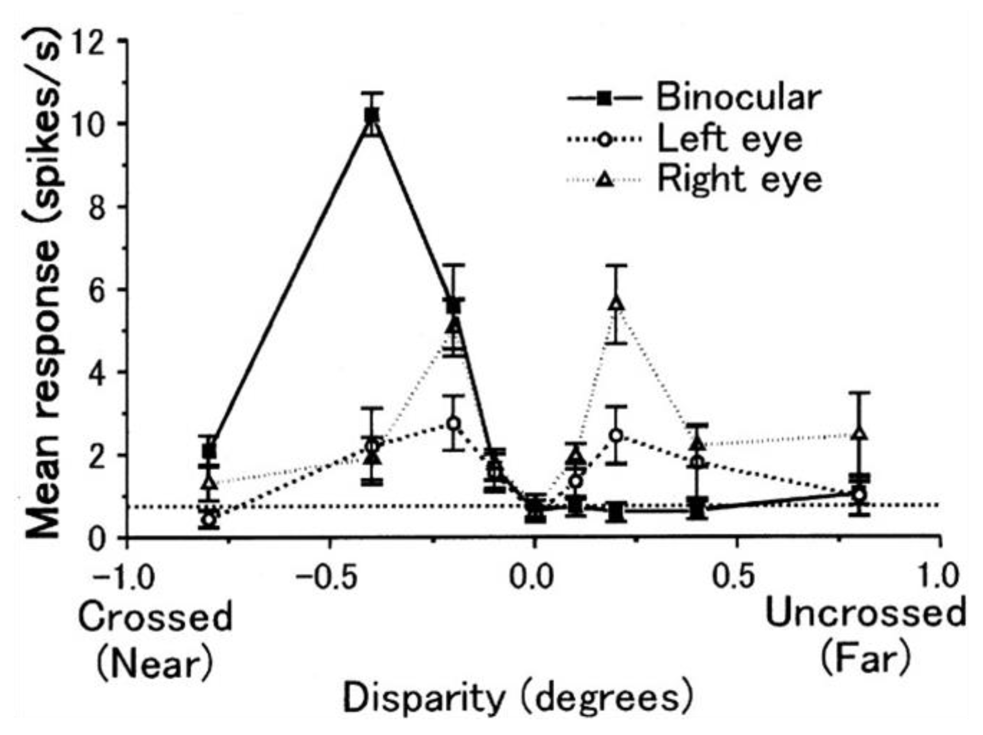
The distance estimation system is based on the study explained in the introduction section, using specialized neuron populations to distinguish between near and distant objects from the binocular system.

To achieve this goal, and due to the above explanation, the projective space of both retinas is split into horizontal stripes, with each one representing a neuron population specialized in a particular projective space. Thanks to this specialization, each neuron population is focused on obtaining the disparities exclusively in its corresponding area, eliminating the noise caused by the other stripes and, thus, obtaining a more accurate distance estimation inside their space.

In this subsection, two mechanisms are explained. The first one represents a general distance estimation based on a global disparity calculation (with no neuron specialization). Further, after that, a second mechanism uses the global estimation to discretize the neurons’ population which may calculate the distance and inhibits the output of other populations. This mechanism cancels the noise produced by the activity from the other stripes, obtaining a fine-grained estimation mechanism with a more reliable result. However, there are some problems that must be solved, because the global disparity calculation may give similar results with near and far objects. For this purpose, a winner-take-all neuron is used [20].

2.2.1. Global Disparity Calculation

At this point, all the hardware components and their calibration have been presented, and then, the distance estimation process is explained next. Summarizing, and emphasizing on what has been explained before, this mechanism consists of obtaining the disparity map of the scene, which is based on the subtractive fusion of the projection from both retinas.

However, spiking vision systems do not provide information in the same way as conventional cameras do: while traditional cameras give information about the scene in static frames (that codify the information during a particular period of time), spiking sensors provide brightness variations of the scene (movements) for each pixel asynchronously (without integrating the information in frames like conventional cameras do). Hence, the information from each retina corresponds to a spike flow with information that is codified as pixel addresses (x and y coordinates) and their corresponding spiking rate (intensity of the variation); but this information is transmitted without following a specific order—that is, asynchronously.

The main difficulty of this processing system is finding a mechanism capable of performing the subtraction operation between two spiking signals. Regarding this problem, Jiménez-Fernández [21] provided the basic building blocks to operate with spiking signals. In that study, some basic components implemented in Hardware Description Language (HDL) were developed, which form the so-called “spiking algebra”. Among these essential components, the “Hold&Fire” block (H&F) is included, with behavior that is equivalent to a spiking signal subtractor.

This block consists of two inputs (signals to be subtracted) and one output (subtraction result). Every time a new spike arrives, it is stored internally, waiting for the evolution of the inputs for a fixed amount of time (hold time). If no spike arrives after this hold time, the stored spike is triggered (sent through the output). However, if a new spike arrives, the one that is stored can be triggered, retaining a new spike; or cancelled, without producing any output and without retaining any spike, depending on which of the two inputs the spike has arrived from. Its functionality is described in Equation (1). So, subtracting a spike-based input signal ($f_U$) to another ($f_Y$) will generate a new spike signal with a spike rate ($f_{SH\&F}$) that will be the difference between both input spike rates.

$$f_{SH\&F}=f_U-f_Y$$

(1)

The functionality of the H&F is to hold the incoming spikes during a fixed period of time while monitoring the input evolution to decide which spike to output, holding, cancelling, or firing spikes according to input spike ports and polarities.

This H&F block was designed for motor control, and so it only contemplates two input signals and two possible states for each of them (positive or negative). In our case, the input signals are related to specific pixels of the retinal projections and, therefore, they also contemplate positive and negative events (increase or decrease in the brightness of the scene, respectively). This fact is closely related to the different types of spikes that occur in the neurons of the human binocular system (excitatory and inhibitory spikes caused by neurons located in the iris).

However, in this work, it is necessary to contemplate information concerning the retina (left or right), since, for the purpose of the spiking subtraction operation, it behaves in an opposite way whether it is a left retina spike or a right retina spike. This behavior was not necessary to be considered in the basic H&F operator, since it contemplated specific lines for each input. In our case, it is not possible to carry it out in that way due to insufficient hardware resources (128 × 128 × 2 inputs would be needed).

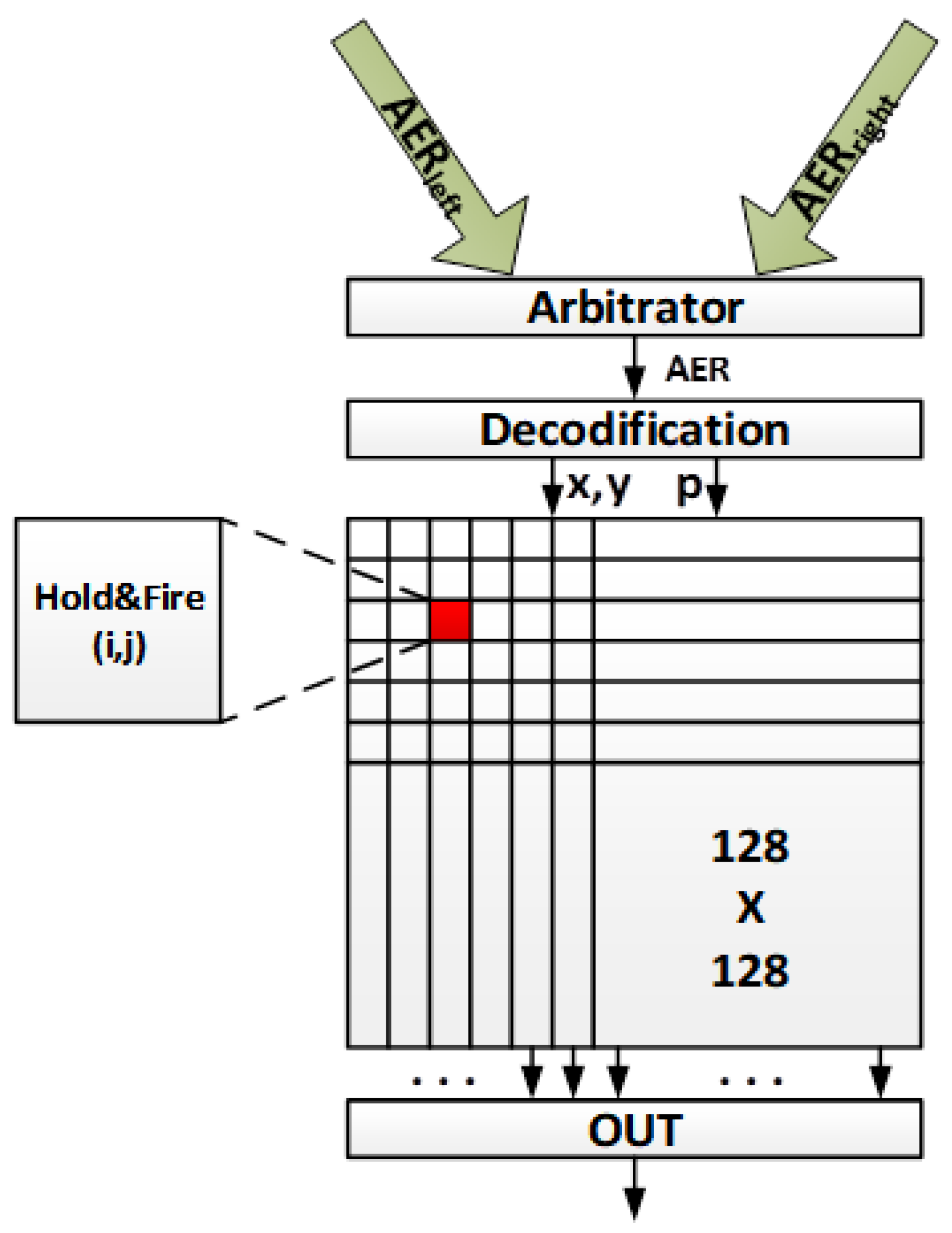
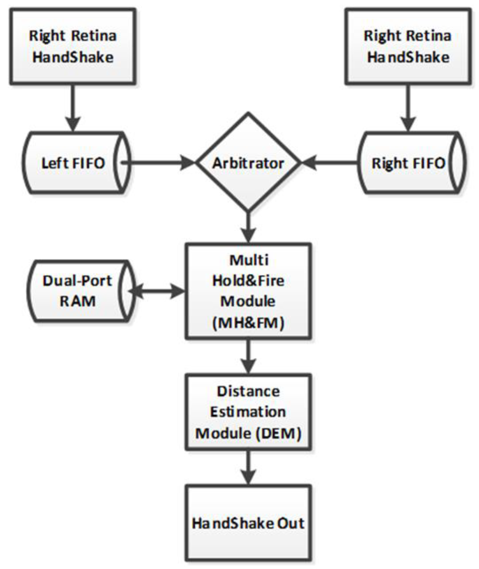
To do that, a new Multi-Hold&Fire (MH&F) was implemented for this work, which was tested in previous works [22]. Its functionality is based on the H&F module but, in this case, it is extended to a 128 × 128 matrix, storing the subtraction data for each pixel (see Figure 4). MH&F bases its functionality on the ampliation of H&F block to the 128 × 128 spike signals produced by the retinas. Each retina has a resolution of 128 × 128 pixels and outputs a spiking signal using an address–event–representation (AER) bus related to the addresses of the pixels that have been fired and whose information is codified in frequency. So, the FPGA can discretize the pixels that have been fired in each retina. Once it receives the information, the address is used as a pointer to the H&F block (inside the MH&F module) where this spike goes. The two signals indicated above for each H&F block are one specific pixel from the right retina and the same pixel from the left retina. All the spikes fired by the 128 × 128 H&F blocks are unified by the MH&F module as one single output, representing its final spike rate.

The information from the spikes received in this module is stored internally in the FPGA in a dual-port memory. The information stored for each pixel is the current state (if it has a retained spike or not), the retina from where the spike comes from (right or left retina) and the spike polarity (positive/excitatory/ON or negative/inhibitory/OFF). Thus, the amount of memory needed is only 6 KB for storing the “disparity map” of the currently displayed scene.

Summarizing the MH&F module behavior, if two spikes coming from the same address of each projection (same pixel) have the same polarity and belong to different retinas, the algorithm will cancel both spikes with each other as long as it does not exceed the retention time initially established between the arrival of both spikes. On the other hand, when both spikes come from the same retina, the opposite behavior occurs and they are cancelled only if they have different polarizations (and the retention time is not exceeded). The full functionality is described on

Table 1. Multi-Hold&Fire truth table. Symbol Ø indicates that no spike is retained (“Retained” column) or no spike is outputted (“Output” column).

1st Spike		2nd Spike		Retained		Output
Retina	Sign	Retina	Sign	Retina	Sign	Retina	Sign
R	+	R	+	R	+	R	+
R	+	L	+	Ø	Ø	Ø	Ø
L	+	R	+	Ø	Ø	Ø	Ø
L	+	L	+	L	+	L	+
R	-	R	-	R	-	R	-
L	-	R	-	Ø	Ø	Ø	Ø
R	-	L	-	Ø	Ø	Ø	Ø
L	-	L	-	L	-	L	-
R	+	R	-	Ø	Ø	Ø	Ø
L	+	R	-	R	-	L	+
R	+	L	-	L	-	R	+
L	+	L	-	Ø	Ø	Ø	Ø
R	-	R	+	Ø	Ø	Ø	Ø
L	-	R	+	R	+	L	-
R	-	L	+	L	+	R	-
L	-	L	+	Ø	Ø	Ø	Ø

.

As detailed in the H&L module, this new module has also a hold time and, after it, the information stored in a cell is reset. As the implementation of the MH&F module is based on a H&F array, the hold time of each cell is controlled independently.

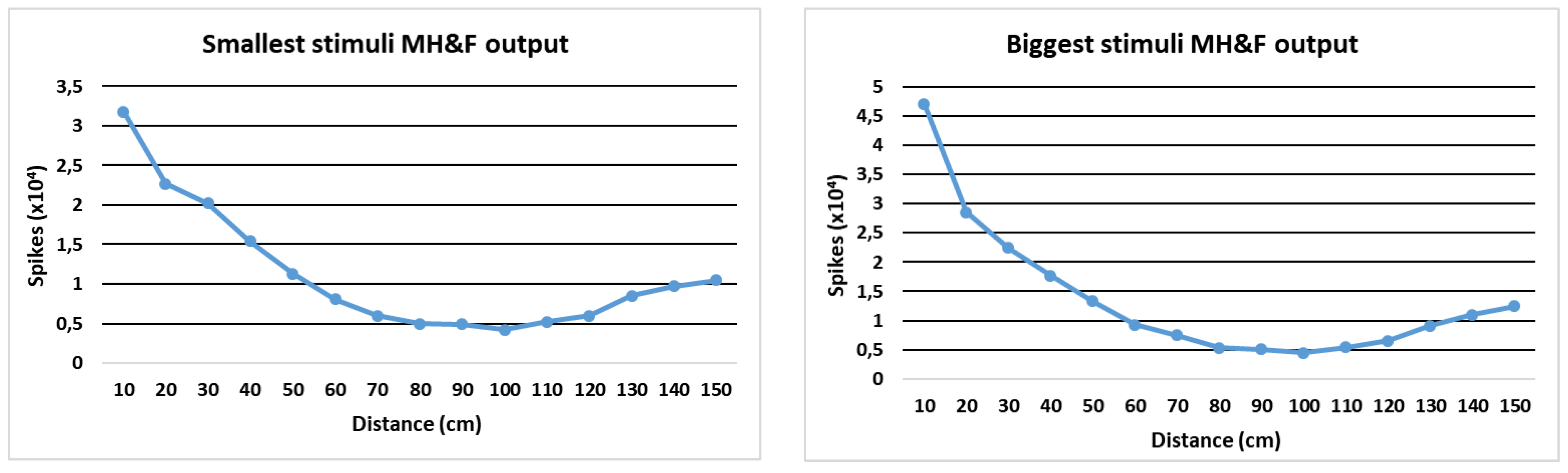
In the human binocular system, distance estimation is related to the process of calculating disparities. In fact, since the neuronal system works with spikes, this distance estimation consists of the spike frequency. So, theoretically, the human binocular system and the MH&F module implemented seem to work in a similar way. With this conclusion, the process of calculating disparities has been solved with the MH&F module, which provides a spiking output with an output frequency related to the disparities of the scene. If both projections are similar, the spike frequency at the output will be very low, while a high spike frequency means that there are many disparities in the scene. In addition, this is related to the physical calibration that was performed in the previous section, where the retinas were placed focused at a distance of 1 m. This way, if the object is above the focus point, the disparities will be minimum. According to the frequency response, a distance estimation can be implemented.

In the results section, the system is characterized using objects at different distances in order to verify this behavior and assign frequency values to the different distances. The module denoted as “distance estimation module” in Figure 5 is calibrated after those tests.

The global distance estimation system depends on the frequency response of the disparity calculation output (after a normalization step). The solution obtained, although acceptable as a coarse-grain estimator, needs another support system to make distance estimation more accurate. This second system is detailed below.

2.2.2. Local Disparity Calculation with Population Inhibition

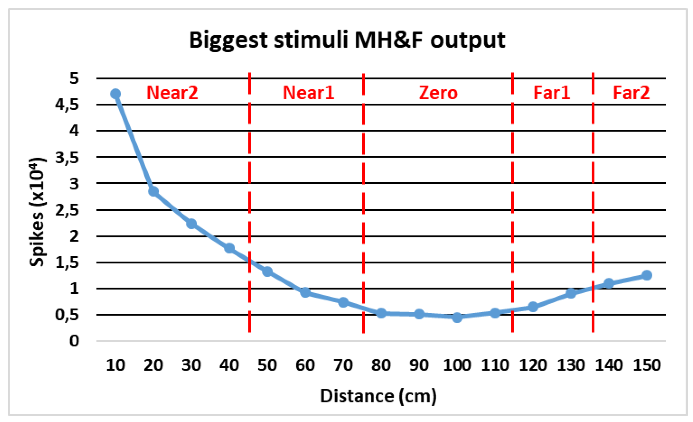
As detailed in the introduction section, distance-estimation neurons are specialized by independent populations. To implement these populations according to the human binocular system functionality, our system divides the projective space into horizontal bands (each one corresponds to a different neuron population). Those horizontal bands closest to the inner areas of the projective space of both retinas correspond to the populations of nearby neurons, while those closest to the outer zones are populations of distant neurons. On the other hand, the most central band of both retinas corresponds to the population of near-to-zero neurons.

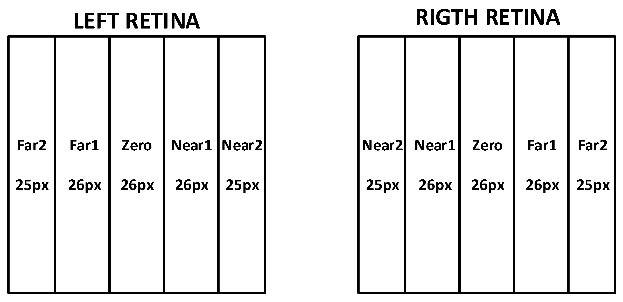
In order to verify the viability of this system and not cause an excessive segmentation of the projective space, it has been divided into five bands (neuron populations): Near2, Near1, Zero, Far1 and Far2. This segmentation is shown in Figure 6. Regarding the size of each band and based on the neuronal specialization of the human binocular system, an equitable division of the horizontal projective space has been used. Thus, Near2 and Far2 bands have a width of 25 pixels, while Near1, Zero and Far1 bands have a width of 26 pixels.

As explained in the previous section, the main aim for this neuronal specialization is to improve the distance estimation accuracy of the full system. Although using the global estimation module exclusively (previous subsection) provides a distance estimation, using neuronal specialization based on a band segmentation improves its accuracy. So, the global distance system works like a coarse-grained estimator, while the neuronal specialized one works like a fine-grained estimator.

Each pair of corresponding bands (the same band from both retinas) carries out a disparity calculation process exclusively in their own projective space (using a MH&F module adapted to their size), obtaining a particular spikes frequency as output (depending on the disparities detected). In this way, the system has six spike flows: the first coming from the global estimation module outcome, and the one coming from each of the five specialized populations described before.

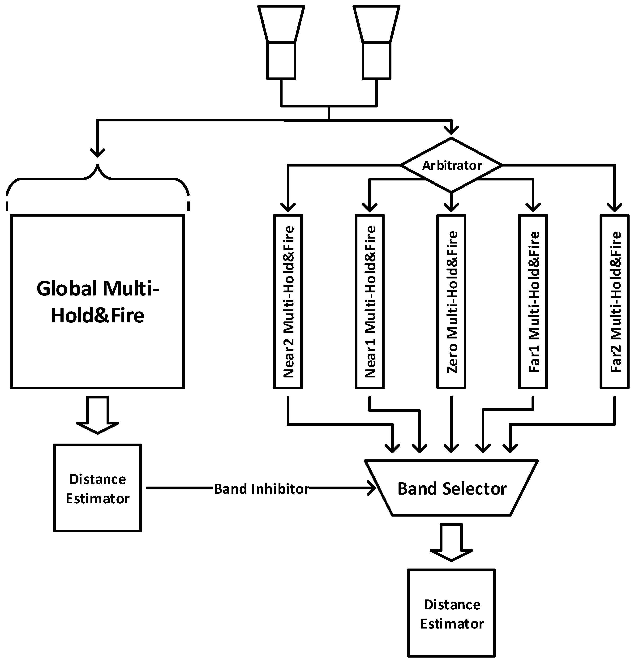
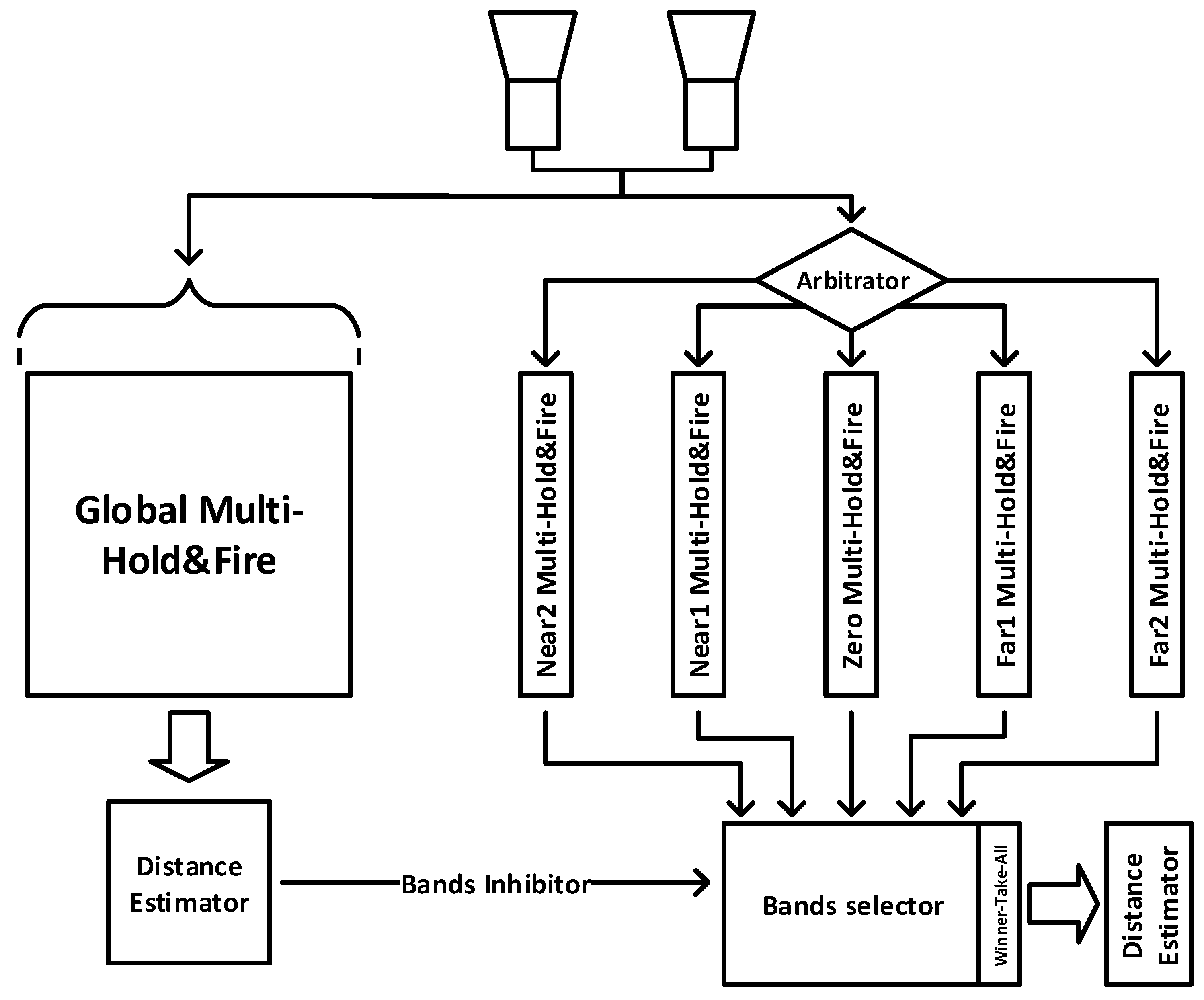
The global estimation system works as an arbiter to select the neural population where most spike traffic is focused. This system inhibits the outflow of the neuronal populations that do not intervene and allows the active population to send its outcome to the final distance estimator module. Once the active neuron population is selected, the final distance estimation module is carried out. So, the last distance estimation module is focused only on the projective space of the active band, ensuring that the noise coming from the rest of the bands does not intervene. The general functionality of the system is shown in Figure 7.

The final functionality is described step by step:

-

Retinas transmit spikes to the FPGA.

-

The FPGA stores the information in FIFOs to avoid losing the information.

A general arbitrator takes each spike from the FIFOs and sends it to both systems: the global Multi-Hold&Fire is shown to the left in Figure 7 and the local disparity calculation is shown to the right in Figure 7.

  ○

In the Global Multi-Hold&Fire, the spike is stored in the 128 × 128 matrix indicated in Figure 4. The functionality of this module is described in Section 2.2.1.

  ○

In the Local side of the processing system, the spike is processed by an internal arbitrator, which sends it to the specific band where it belongs. Each band works like a Multi-Hold&Fire module but only with the spikes belonging to the band itself.

-

Each Multi-Hold&Fire module (Global, Near2, Near1, Zero, Far1 and Far2) outputs the difference of the information from each retina inside the projection space where it is working (the whole space for the Global module, but only a specific band for the local modules).

-

Distance estimator outside the Global module discretizes the band within the object in movement thanks to the spiking frequency obtained outside the Global module. This inhibitor acts like a band selection of the Local part of the system.

-

Once the specific band is selected, the spike frequency obtained by itself (using the Multi-Hold&Fire with the spikes within its projection space) is sent to the final distance estimator. This estimator, according to the spike frequency, determines the final estimation of the moving object.

The thresholds used to determine the distance where the object is located (to inhibit the other bands) are calculated based on the characterization tests presented in the next section. This process reflects an important problem that is detailed deeply in the next section: some bands give similar frequency outputs for some objects, and so we need another module to intervene in the inhibitory process (this module is not included in Figure 7 but will be included next).

After that, the results of the fine-grained system functionality (with the specialized neuronal populations) are compared to the coarse-grained one.

3. Results

This section is divided into two parts. First, some tests are carried out with moving objects at specific distances from the stereoscopic system. These tests are used to characterize the system, obtaining the thresholds values for both distance estimation systems, as well as to demonstrate the system’s response similarity with the human binocular system.

Secondly, the system is integrated in a real-time environment, so that we can check the speed of the response in addition to the accuracy of the distance estimator.

In both cases, a comparison is made between the coarse-grained system and the fine-grained one, to show neuronal specialization improvement.

3.1. System Characterization Tests

For these tests, a controlled laboratory environment is established, with a uniform background and natural light (to avoid flickering of the fluorescent tubes that cause malfunctions in the neuromorphic retinas). By carefully controlling the distance, five objects (with different sizes and shapes) are moved laterally (maintaining the distance from the vision system and without moving far away from the central convergence axis). For each singular distance (from 10 to 150 cm), the system output is recorded for exactly 10 s using jAER software developed by Delbrück, T.

The results for the smaller and bigger objects are shown in Figure 8 left and right, respectively. The graphical representation is shown (to compare it with the human binocular system) and a table with the numerical values is presented to check the spikes rate for obtaining the threshold values (

Table 2. Multi-Hold&Fire spikes rate for the smallest object experiment.

Distance (cm)	10	20	30	40	50	60	70	80	90	100	110	120	130	140	150
Spikes (×104)	3.18	2.27	2.02	1.54	1.13	0.81	0.65	0.50	0.49	0.42	0.52	0.60	0.85	0.97	1.05
Spikes/s (×104)	0.32	0.23	0.20	0.15	0.11	0.08	0.06	0.05	0.05	0.04	0.05	0.06	0.08	0.10	0.11
Spikes/20 ms	64	46	40	30	22	16	12	10	10	8	10	12	17	20	21

for the smallest object and

Table 3. Multi-Hold&Fire spikes rate for the biggest object experiment.

Distance (cm)	10	20	30	40	50	60	70	80	90	100	110	120	130	140	150
Spikes (×104)	4.71	2.85	2.24	1.77	1.33	0.93	0.75	0.53	0.51	0.45	0.54	0.65	0.91	1.10	1.25
Spikes/s (×104)	0.47	0.28	0.22	0.17	0.13	0.09	0.07	0.05	0.05	0.04	0.05	0.06	0.09	0.11	0.13
Spikes/20 ms	94	56	44	34	26	18	15	10	10	9	10	13	18	22	25

for the biggest object). The tables show the integration of the spikes during the 10 s of sampling (second row), the equivalent spikes per second (third row) and the spikes at the output for 20 milliseconds. This last value is used for the threshold estimation, since the distance estimation module integrates the output spikes every 20 milliseconds in order to obtain approximately 50 outputs per second (without taking into account the initial delay of the components, which can be negligible once it starts working).

In both cases, the closer the object is to the vision system, the higher the output is. In the same way, the lowest event rate at the output of the Multi-Hold&Fire module is located in an environment close to the focus point (100 cm). These facts corroborate the theoretical study carried out initially and certify the feasibility of using this system to estimate distances of moving objects along the central convergence axis.

If we compare the response obtained after these tests with the human binocular system response, the study conducted by Uka and Yoshiyama [23] shows the output frequency given by the output of the visual neurons disparity operation with a stimulus located at several distances from the focus point (see Figure 9). If we compare this study with the previous results, a great similarity can be observed regarding the disparity system’s output behavior. So, we can affirm that the system proposed in this work imitates the processing carried out by the visual neurons responsible for the disparity process in the human binocular fusion.

On the other hand, analyzing the quantitative results, some important facts can be obtained:

• The object size practically does not intervene in the spike disparity output rate. In fact, where the disparity result is better obtained (closed to the focus point), the output spike disparity frequency is practically identical (no matter the size of the object, if the subtraction is going to be almost zero). This fact indicates that thresholds can be used for any object.
• Based on the physical band segmentation indicated in the previous section, the distance division for each zone is performed: [10.50), [50.80), [80,110], (110,130] and (130,150].
• The Zero zone range (between 80 and 110cm) and the Near2 zone (less than 50cm) can be distinguished perfectly by thresholds. Hence, the global distance estimation process will be accurate when the object is in those positions.
• However, in certain bands the output spike frequency is similar. For example, for nearby (but not very close) positions, the spikes rate is similar to the one obtained in distant positions. This is a problem for the inhibition process carried out by the global distance estimation system. Therefore, for integration with the fine-grained system, it is necessary to add a winner-take-all [20] module that, given the possibility that the object is in more than one band (due to similar threshold values), it could be selected using is the highest spike frequency obtained at the output of each band.

Following these considerations, the threshold values that are established are indicated in Figure 10 (corresponding to the biggest object) and in

Table 4. Thresholds.

Band	Near2	Near1	Zero	Far1	Far2
Distance (range)	[10, 50)	[50, 80)	[80, 110]	(110, 130]	(130, 150]
Thresholds (spikes/20 ms)	>30	(30, 12)	<12	(12, 20)	(20, 30)

.

As presented above, there are some distances with frequency responses that are very similar and, therefore, this general system would not know how to distinguish between them: this is the case with the Near1, Far1 and Far2 bands. To solve this problem, the only way to distinguish it is by observing the frequency response of each population independently: therefore, to the discretization made by the global system, a winner-take-all system is added for doubtful cases. So, it is used to select the band with the highest spikes frequency after the disparity calculation process.

After this modification, the final system can be seen in Figure 11. The functionality of the final system (see Figure 11) is similar to the one described in Figure 7, but it has some differences:

-

The distance estimator outside the Global module discretizes the band in the same way as described in Figure 7. However, the result of this estimator may have more than one band. This information of the bands selected is transmitted to the band selector module.

-

The band selector inhibits the outputs of the bands not selected. The information obtained from the other bands is evaluated according to their spike frequency in the winner-take-all module. This module checks their frequency from all the inputs and selects the higher frequency as the “winner”, inhibiting the others.

-

Finally, the final distance estimator uses the frequency received by the winner-take-all module and estimates the distance where the moving object is (inside the limits of the “winner” band).

To evaluate its efficiency and improvement compared to the global estimation system exclusively, the data collected by each stimulus is divided into files of 20 ms duration, obtaining 500 samples for each object and distance (2500 samples for each distance). Each of them is used as input for the final system (global estimation and winner-take-all module for the inhibition process, and neuronal specialization for fine-grained distance estimation) and the distance estimation errors are obtained. These results can be seen in

Table 5. Characterization test results obtained with the global distance estimator (Section 2.2.1) are shown in rows 2–5. Results obtained with the neuronal specialization system (Section 2.2.2) are shown in rows 6–9. The comparison is shown in rows 10–11.

	Distance (cm)	10	20	30	40	50	60	70	80	90	100	110	120	130	140	150
Global System	Success	1362	1791	1905	1879	1313	1381	1146	1775	1670	1903	1488	1397	1249	1327	1591
	Failures	1138	709	595	621	1187	1119	1354	725	830	597	1012	1103	1251	1173	909
	Error (%)	45.52	28.36	23.80	24.84	47.48	44.76	54.16	29.00	33.2	23.88	40.48	44.12	50.04	46.92	36.36
	Mean Error (%)	38.19466667
Full System	Success	2293	2319	2303	2345	2198	2256	2284	2353	2322	2411	2287	2172	2189	2230	2215
	Failures	207	181	197	155	302	244	216	147	178	89	213	328	311	270	285
	Error (%)	8.28	7.24	7.88	6.20	12.08	9.76	8.64	5.88	7.12	3.56	8.52	13.12	12.44	10.80	11.40
	Mean Error (%)	8.86
	Improvement	40.60	22.77	17.28	19.87	40.26	38.79	49.82	24.56	28.08	21.07	34.94	35.68	42.94	40.49	28.17
	Mean Improvement	32.35

.

Results (see Table 5) show that the success rate for the neuronal specialized system is higher than 91% (rows 6–9 of Table TTT2) using the discrete distances between 10 and 150 cm. These results are represented for each particular distance, with an 8.86% mean error. If we compare those results with the global estimation system alone (rows 2–5 of Table 5), we obtain great improvement (32.35%: see row 11 of Table 5). These results demonstrate the correct functioning of the distance estimation system with neuronal specialization and prove that this neuronal specialization system is needed in order to obtain good results.

3.2. Real-Time Test

To perform a real-time test, a Scalextric kit has been used. Its path is located over the optical convergence axis of the stereoscopic vision system. The assembly involves a straight-line section (just over 1 m long), and two circular sections so that the vehicle repeats the main route again without interruption. In this way, constant stimulus is achieved, and it is easier to evaluate the results and the distance estimation.

In order to keep the car in constant movement without using a user to manually control the vehicle controller, a new module based on a microcontroller and an engine control board is used. With this module and a developed user application, the vehicle speed can be quantitatively controlled, and it becomes constant over time. The block diagram of the additional system used is shown in Figure 12.

The stereoscopic vision system is placed at one end of the circuit with the FPGA and the connections to the computer. This assembly is shown in Figure 13.

On the other hand, a LED array is added to the side, which will be used to validate the system functionality. The LEDs of this array are separated by exactly 10 cm and are positioned at the exact distances of the points used for the characterization tests. Due to the size of the Scalextric and its arrangement, it is not possible to cover all the distances used in the previous section, finally obtaining a range of 40–120 cm (considering all the neurons’ bands implemented in the system).

The system implemented in the FPGA in the one described in Figure 11 with an important modification: the Local estimation system is only divided into three bands because of the Scalextrik and hardware limitations. The distance that the car travels in straight line goes from 40 to 120 cm, so the bands described in Section 3.1 that contemplates these distances are Near1, Zero and Far1.

The tests are performed with 10 different speeds of the vehicle, making a recording with a conventional camera located on the side of the circuit during 30 s per speed value. Subsequently, all videos are played in slow motion in the computer and the lighting of each LED is checked as the vehicle runs parallel to it. For speed 1, the vehicle performs two full turns to the circuit and four for speed 2, eight for speed 3, etc. For each turn, two estimations for each distance are obtained (forward and backward). So, finally, 220 estimations for each distance are evaluated. Based on these manual checks, the statistics of successes and failures in the distance estimations are obtained.

These tests have been performed for the initial global system version and for the system with neuronal specialization, obtaining both results to compare them.

Some screenshots are shown in Figure 14 while the vehicle is moving.

Table 6. Real-time test results obtained with the global distance estimator (Section 2.2.1) are shown in rows 2–5. Results obtained with the neuronal specialization system (Section 2.2.2) are shown in rows 6–9. The comparison is shown in rows 10–11.

	Distance (cm)	40	50	60	70	80	90	100	110	120
Global System	Success	137	107	123	113	121	134	149	63	49
	Failures	83	113	97	107	99	86	71	157	171
	Error (%)	37.72	51.36	44.09	48.63	45.00	39.09	32.27	71.36	77.72
	Mean Error	49.69
Full System	Success	193	185	169	177	199	202	196	182	178
	Failures	27	35	51	43	21	18	24	38	42
	Error (%)	12.27	15.90	23.18	19.54	9.54	8.18	10.90	17.27	19.09
	Mean Error	15.10
	Improvement (%)	29.02	42.16	27.22	36.16	39.20	33.66	23.98	65.38	72.47
	Mean Improvement	41.02

shows the results obtained for each of the distances and for each of the systems tested. It can be observed that the neuronal specialization system obtains better results than the global estimator while the vehicle is moving (improving the results in a 41%).

With real-time tests the error increased for all the systems tested. The neuronal specialized estimator obtains a 15.10% error (almost double that the error obtained with the characterization tests), but the results are good enough for a distance estimator.

As can be observed in Table 6, the results are discretized by 10 cm stripes. There are several reasons that justify this decision and they are explained below:

-

First, the human binocular system estimates distances, which is not the same as calculating them. Thus, since this work imitates its operation, this uncertainty has been transferred to the tests. However, the results show that the error obtained is acceptable.

-

On the other hand, these stripes are related to the calibration distances used during the characterization tests. Using more stripes in the results does not allow us to compare them with the characterization results.

-

Moreover, using more calibration distances in the characterization tests has problems too. The retinas used, as explained above, are only able to detect moving objects. So, during the characterization tests, the information obtained from the retinas may have errors. If we use, for example, distances of 2.5 cm, during the movement of the object (needed to collect data) the information obtained is not exactly at this distance (it could approach the next calibration point). So, the system would be calibrated with data that is not completely correct from the beginning and, because of this, we cannot obtain good results in the final tests.

Due to this explanation, the system resolution has been estimated experimentally. This resolution depends on the bands that intervene in the DEM calculation: the Zero band obtains a better resolution (approximately ± 1.5 cm) than Far bands (approximately ± 2.5 cm). This is caused because of system noise and the object being in movement. Because of that resolution, a specific estimation should not be marked as wrong when the system does not exactly estimate the position. This is added to the delay caused by the microcontroller with the led array which, even though it is small, could mean variations at the millimeter stage because of the vehicle’s movement. Thus, in the real-time experiments, we have considered that an error of ± 2.5 cm is not a wrong estimation. This value has been obtained using the worst resolution indicated in the previous point.

So, it is proved the presented system can be used in a real-time scenario with acceptable results, and these results are improved thanks to neuronal specialization.

All the tests have been detailed and presented. Finally, in the discussion section, these results are be analyzed.

4. Discussion

In this work, a study of the biological model for distance estimation based on the ocular disparities of the binocular system is described. This biological system has been analyzed in depth and previous studies describing its functionality have been detailed.

This study carries out the implementation of a processing module that mimics the binocular disparity estimation in spiking bio-inspired systems. In addition, a system based on two-level processing with neuronal specialization for improvement in distance estimation is detailed. This model is completely based on the human binocular system.

The results obtained demonstrate the similarity between the human binocular system and the system designed in this work, evaluating the results for several tests: characterization and real-time tests. The results obtained exceed 91% success with the characterization tests and represent 85% success in the tests with the real-time system.

These results allow the system to run in a real-time environment. The information observed in

Table 7. Estimated FPGA power consumption of full system implementation running with an input of 2 Mevps.

On-Chip Power	Consumption (mW)	From Total (%)
Dynamic	2	2.06
- Signals	0.67	0.68
- Logic	1.09	1.12
- Input/Ooutput	0.24	0.26
Static	96	97.94
Total	98	100

shows that out system has a power consumption of 0.98 Watts, while a desktop computer needs more than 50 Watts. So, our system can be executed in an FPGA with power consumption that is much lower than the equipment needed to perform this task using digital cameras with classic computer vision.

References

1. Andrew, A.M. Multiple View Geometry in Computer Vision. Kybernetes; Cambridge University Press: New York, NY, USA, 2001. [Google Scholar]
2. Dyer, C.R. Volumetric scene reconstruction from multiple views. In Foundations of Image Understanding; Springer: Boston, MA, USA, 2001; pp. 469–489. [Google Scholar]
3. Dominguez-Morales, M.J.; Jimenez-Fernandez, A.; Jimenez-Moreno, G.; Conde, C.; Cabello, E.; Linares-Barranco, A. Bio-Inspired Stereo Vision Calibration for Dynamic Vision Sensors. IEEE Access 2019, 7, 138415–138425. [Google Scholar] [CrossRef]
4. Dominguez-Morales, M.; Domínguez-Morales, J.P.; Jiménez-Fernández, Á.; Linares-Barranco, A.; Jiménez-Moreno, G. Stereo Matching in Address-Event-Representation (AER) Bio-Inspired Binocular Systems in a Field-Programmable Gate Array (FPGA). Electronics 2019, 8, 410. [Google Scholar] [CrossRef] [Green Version]
5. Douret, J.; Benosman, R. A volumetric multi-cameras method dedicated to road traffic monitoring. IEEE Intell. Veh. Symp. 2004, 2004, 442–446. [Google Scholar]
6. Mead, C. Neuromorphic Electronic Systems. Proc. IEEE 1990, 78, 1629–1636. [Google Scholar] [CrossRef] [Green Version]
7. Jimenez-Fernandez, A.; Cerezuela-Escudero, E.; Miró-Amarante, L.; Domínguez-Morales, M.J.; de Asís Gómez-Rodríguez, F.; Linares-Barranco, A.; Jiménez-Moreno, G. A binaural neuromorphic auditory sensor for FPGA: A spike signal processing approach. IEEE Trans. Neural Netw. Learn. Syst. 2016, 28, 804–818. [Google Scholar] [CrossRef] [PubMed]
8. Lichtsteiner, P.; Posch, C.; Delbrück, T. A 128x128 120dB 15μs Latency Asynchronous Temporal Contrast Vision Sensor. IEEE J. Solid-State Circuits 2008, 43, 566–576. [Google Scholar] [CrossRef] [Green Version]
9. Diner, D.B.; Fender, D.H. Human Engineering in Stereoscopic Viewing Devices; Springer International Publishing: Berlin, Germany, 1993. [Google Scholar]
10. Schiller, P.H.; Sandell, J.H.; Maunsell, J.H.R. Functions of the on and off channels of the visual system. Nature 1986, 322, 824–825. [Google Scholar] [CrossRef] [PubMed]
11. Poggio, G.F.; Gonzalez, F.; Krause, F. Stereoscopic mechanisms in monkey visual cortex: Binocular correlation and disparity selectivity. J. Neurosci. 1988, 8, 4531–4550. [Google Scholar] [CrossRef] [PubMed] [Green Version]
12. Nelson, J.I.; Kato, H.; Bishop, P.O. Discrimination of orientation and position disparities by binocularly activated neurons in cat striate cortex. J. Neurophysiol. 1977. [Google Scholar] [CrossRef]
13. Hubel, D.H.; Wiesel, T.N. Stereoscopic vision in macaque monkey: Cells sensitive to binocular depth in area 18 of the macaque monkey cortex. Nature 1970, 225, 41–42. [Google Scholar] [CrossRef] [PubMed]
14. Poggio, G. The Analysis of Stereopsis. Annu. Rev. Neurosci. 1984, 7, 379–412. [Google Scholar] [CrossRef] [PubMed]
15. Serrano-Gotarredona, R.; Oster, M.; Lichtsteiner, P.; Linares-Barranco, A.; Paz-Vicente, R.; Gómez-Rodríguez, F.; Camunas-Mesa, L.; Berner, R.; Rivas-Perez, M.; Delbruck, T.; et al. CAVIAR: A 45k neuron, 5M synapse, 12G connects/s AER hardware sensory-processing-learning-actuating system for high-speed visual object recognition and tracking. IEEE Trans. Neural Netw. 2009, 20, 1417–1438. [Google Scholar] [CrossRef] [PubMed] [Green Version]
16. Sivilotti, M. Wiring Considerations in Analog VLSI Systems with Application to Field-Programmable Network; Caltech: Pasadena, CA, USA, 1991. [Google Scholar]
17. Berner, R.; Delbrück, T.; Civit-Balcells, A.; Linares-Barranco, A. A 5 Meps $100 USB2.0 Address-Event Monitor-Sequencer Interface. In Proceedings of the 2007 IEEE International Symposium on Circuits and Systems, New Orleans, LA, USA, 27–30 May 2007. [Google Scholar]
18. Jáuregui-Olazabal, L.A. Fotogametría Básica; Universidad de los Andes: Bogota, Colombia, 2008. [Google Scholar]
19. Banks, M.S.; Read, J.C.A.; Allison, R.S.; Watt, S.J. Stereoscopy and the human visual system. SMPTE Motion Imaging J. 2012, 121, 24–43. [Google Scholar] [CrossRef] [PubMed]
20. Lazzaro, J.; Ryckebusch, S.; Mahowald, M.A.; Mead, C.A. Winner-take-all Networks of O (n) Complexity; Morgan Kaufmann Publishers Inc.: San Francisco, CA, USA, 1989; pp. 703–711. [Google Scholar]
21. Jimenez-Fernandez, A.; Domínguez-Morales, M.; Cerezuela-Escudero, E.; Paz-Vicente, R.; Linares-Barranco, A.; Jimenez, G. Simulating building blocks for spikes signals processing. In Lecture Notes in Computer Science (Including Subseries Lecture Notes in Artificial Intelligence and Lecture Notes in Bioinformatics); Springer: Berlin/Heidelberg, Germany, 2011. [Google Scholar]
22. Domínguez-Morales, M.; Jimenez-Fernandez, A.; Paz, R.; López-Torres, M.R.; Cerezuela-Escudero, E.; Linares-Barranco, A.; Jimenez-Moreno, G.; Morgado, A. An approach to distance estimation with stereo vision using address-event-representation. In Proceedings of the International Conference on Neural Information Processing, Shanghai, China, 13–17 November 2011. [Google Scholar]
23. Uka, T.; Tanaka, H.; Yoshiyama, K.; Kato, M.; Fujita, I. Disparity selectivity of neurons in monkey inferior temporal cortex. J. Neurophysiol. 2000, 84, 120–132. [Google Scholar] [CrossRef] [PubMed]
Figure 1. Hardware platforms: (a) DVS128_PAER retina; (b) USB-AERmini2 monitoring board; (c) Virtex-5 field-programable gate array (FPGA) evaluation board.
Electronics 08 01502 g001
Figure 2. Physical calibration with a 100 cm convergence, obtaining angle α as 86.1387º.
Electronics 08 01502 g002
Figure 3. Stereo DVS128 address–event–representation (AER) system (left) with Virtex-5 FPGA board and USBAERmini2 monitoring board (right).
Electronics 08 01502 g003
Figure 4. Multi-Hold&Fire module.
Electronics 08 01502 g004
Figure 5. VHDL block diagram for the global distance estimation system.
Electronics 08 01502 g005
Figure 6. Band segmentation in both retinas.
Electronics 08 01502 g006
Figure 7. Full system’s block diagram.
Electronics 08 01502 g007
Figure 8. Spikes obtained at the output of the Multi-Hold&Fire (MH&F) module when using the smallest object as stimuli (left) of the biggest object (right).
Electronics 08 01502 g008
Figure 9. Uka and Yoshiyama studies [23]. The disparity output spiking rate (Binocular) has a similar response to the H&F module.
Electronics 08 01502 g009
Figure 10. Graphical representation of the thresholds for the biggest object response.
Electronics 08 01502 g010
Figure 11. Final system’s block diagram with winner-take-all stage.
Electronics 08 01502 g011
Figure 12. Car speed control system.
Electronics 08 01502 g012
Figure 13. Scalextric used for the real-time test.
Electronics 08 01502 g013
Figure 14. Real-time test with Scalextric. Captures can be observed at various distances from the system in real time. As can be seen, the estimate is not always completely correct.
Electronics 08 01502 g014