Masivo: Parallel Simulation Model Based on OpenCL for Massive Public Transportation Systems’ Routes


Abstract
1. Introduction
2. Public Transport Systems’ Basis
- N = total stops;
- R = total routes;
- = OD (Origin-Destination) demand;
- = passenger travel time;
- = round-trip time on route r;
- = frequency on route r;
2.1. Passenger Demand in Public Transport Systems
2.2. Public Transport Vehicle Routes
2.3. Traffic Simulation Software
2.4. Traffic Simulation Parameters’ Specification
2.5. Simulation Performance Indicators
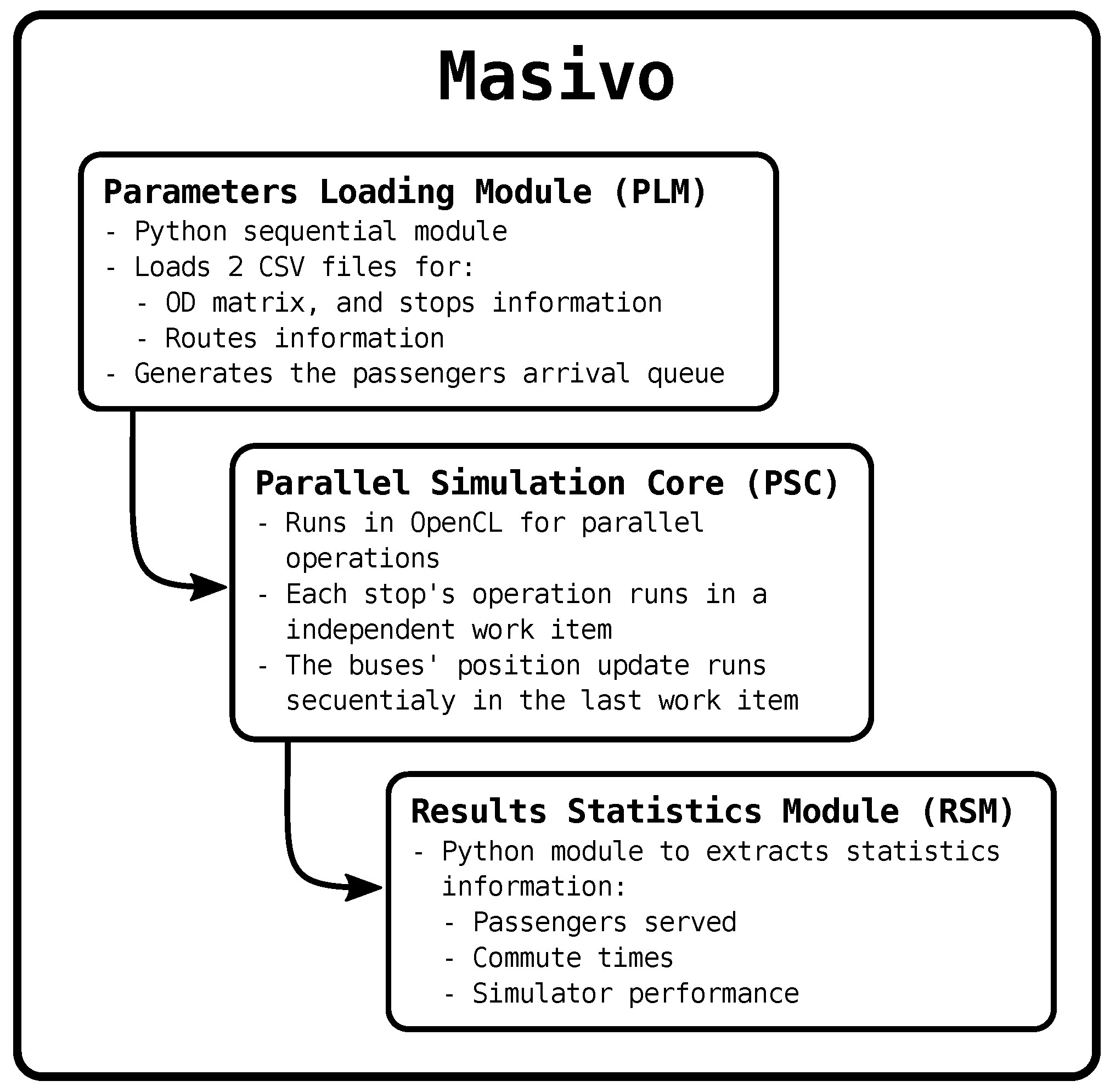
3. Masivo Public Transport Routes’ Simulation
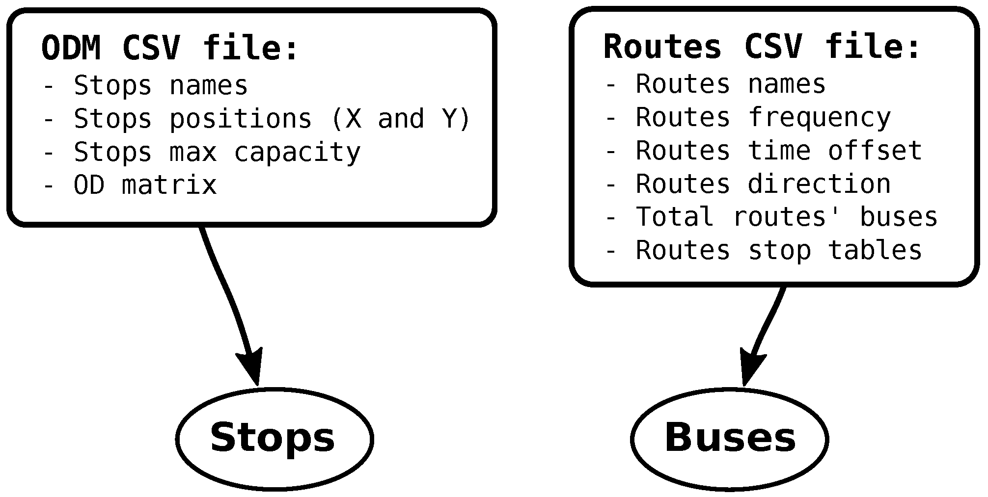
3.1. Parameters Loading Module
3.1.1. ODM CSV File
3.1.2. Routes’ CSV File
3.1.3. Passenger Arrival Queue Generation
| Algorithm 1 Passenger arrival queue generation algorithm. |
|
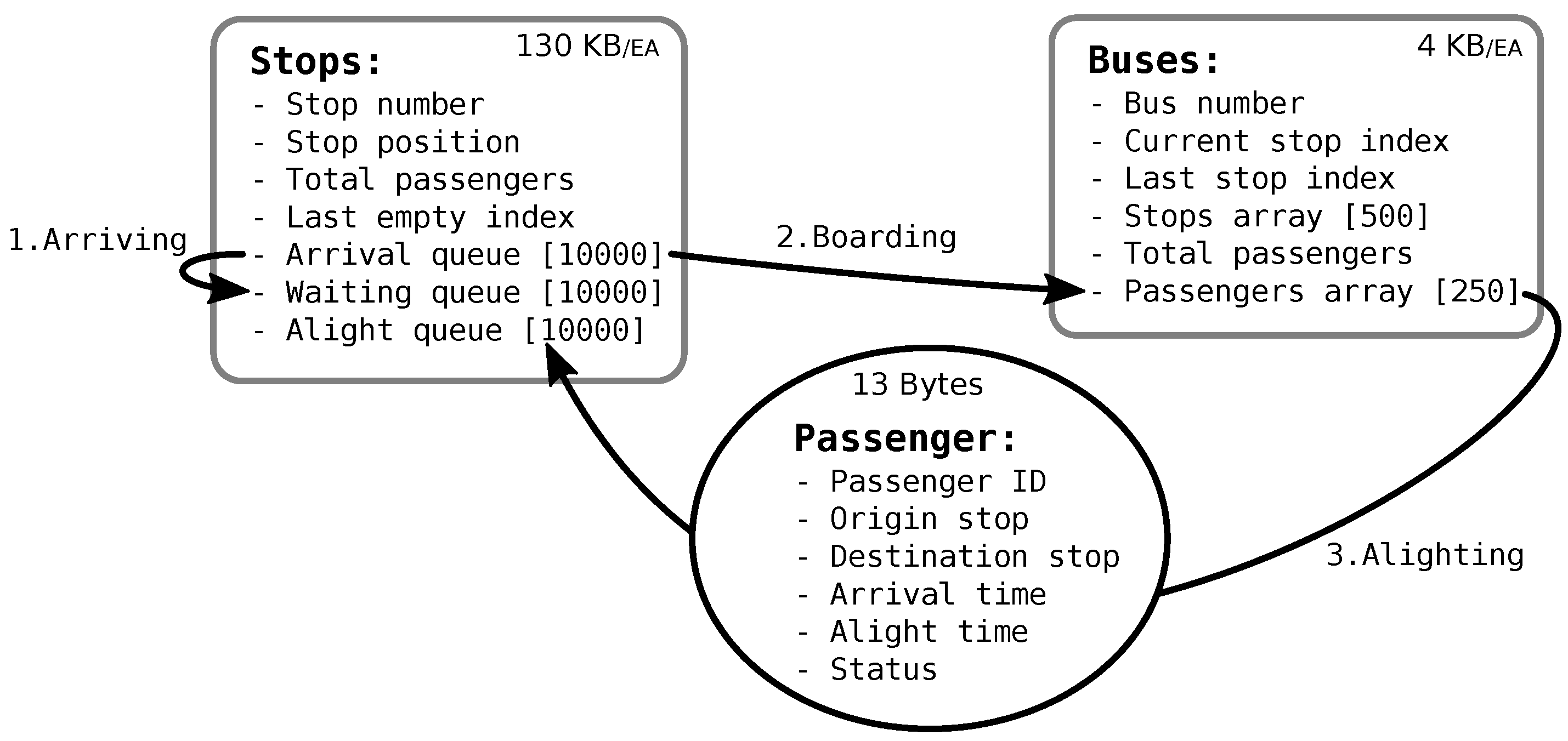
3.2. Parallel Simulation Core
3.2.1. Passenger Arriving
| Algorithm 2 Passengers’ arriving operation at stop n, where passenger arrival queue and passenger waiting queue are specific for stop n. |
|
3.2.2. Passenger Boarding
| Algorithm 3 Passengers’ boarding operation at stop n, where is the passenger waiting queue specific for the stop n. |
|
3.2.3. Passenger Alighting
| Algorithm 4 Passenger alighting operation at stop n, where passenger waiting queue and passenger alight queue are specific for stop n. |
|
3.2.4. Buses’ Position Update
| Algorithm 5 Bus update position operations. |
|
3.3. Results Statistics Module
3.3.1. Passengers Served Information
- total_passengers_results.csv: contains all the information (passenger ID, origin and destination stops, arrival and alight time, and status) of all passengers inside the simulation.
- served_passengers_per_stop.csv: describes per stop the total number of passengers waiting for a bus, the expected total input passengers, the total alight passengers, the total expected alight passengers, and the alighted passengers’ percentage.
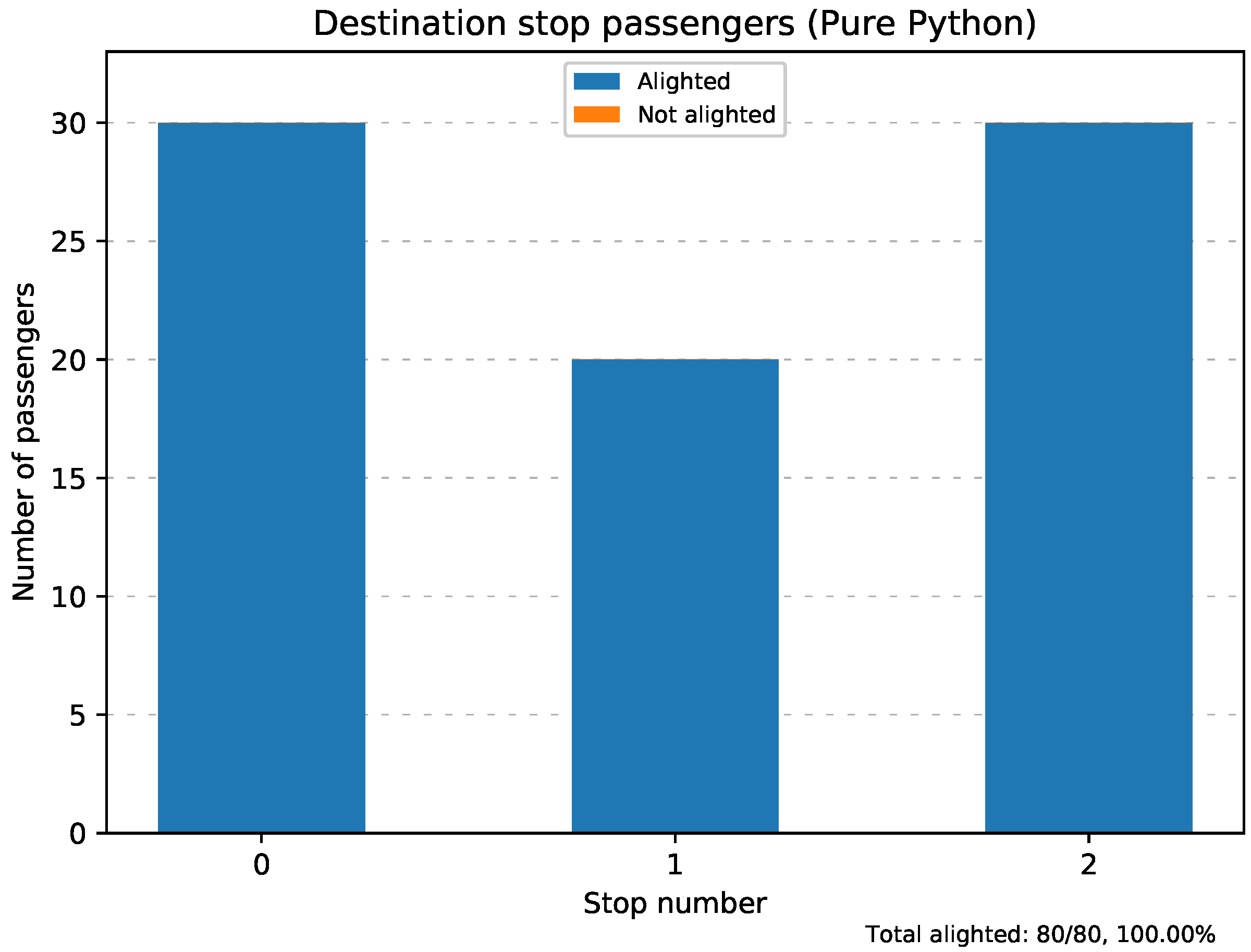
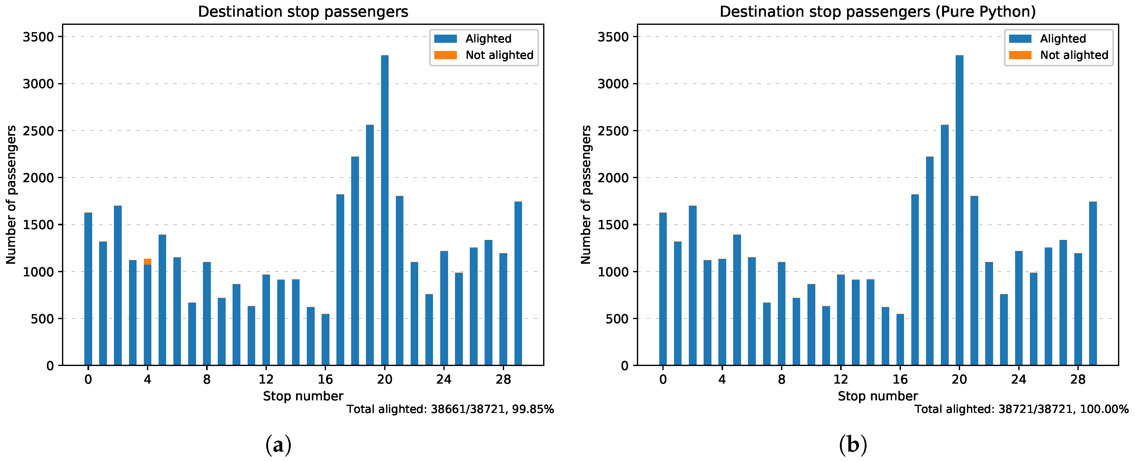
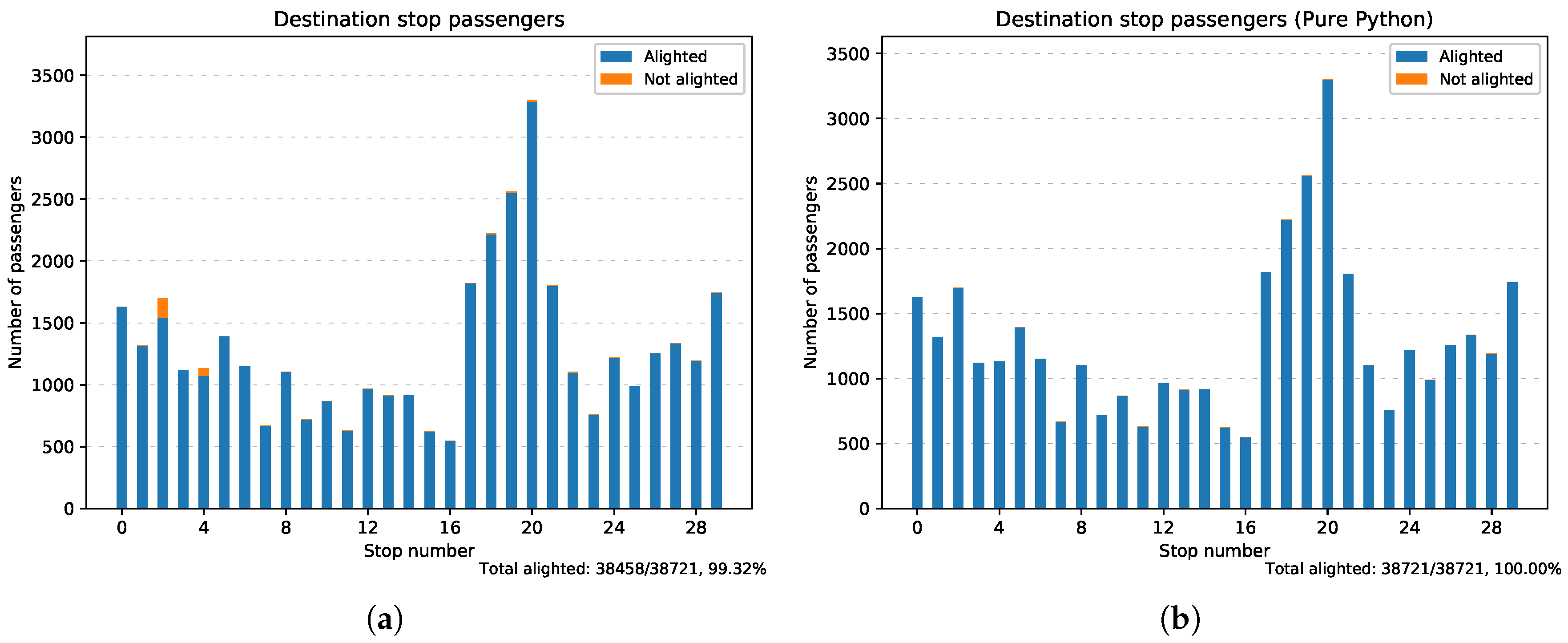
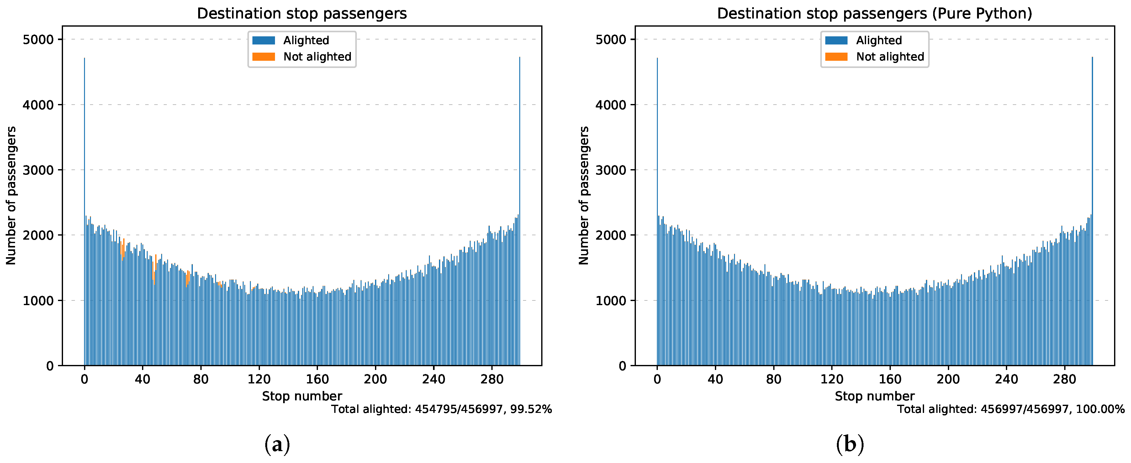
- served_passengers_per_stop.eps: graphs the total alighted passengers contrasted with the remaining passengers expected per stop.
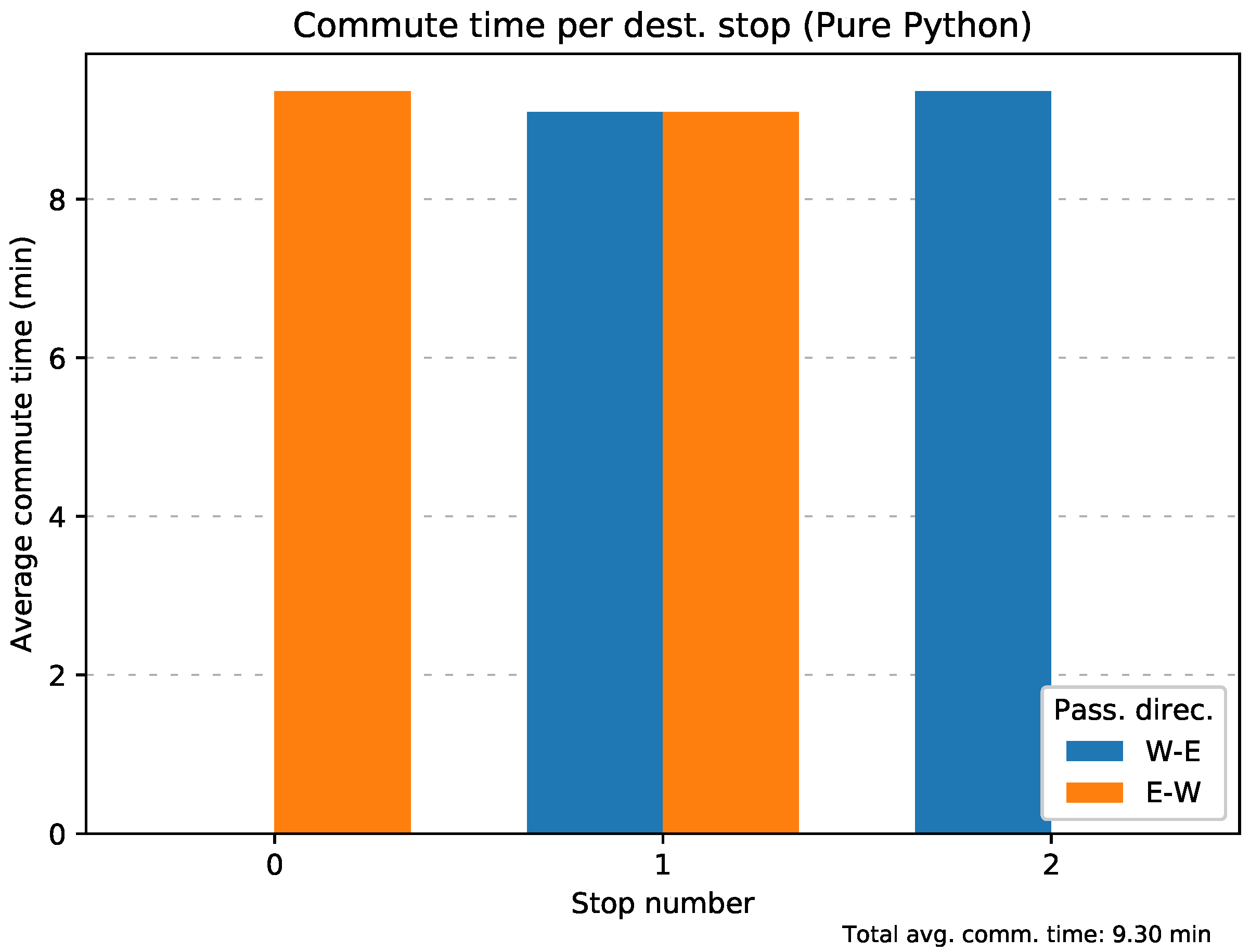
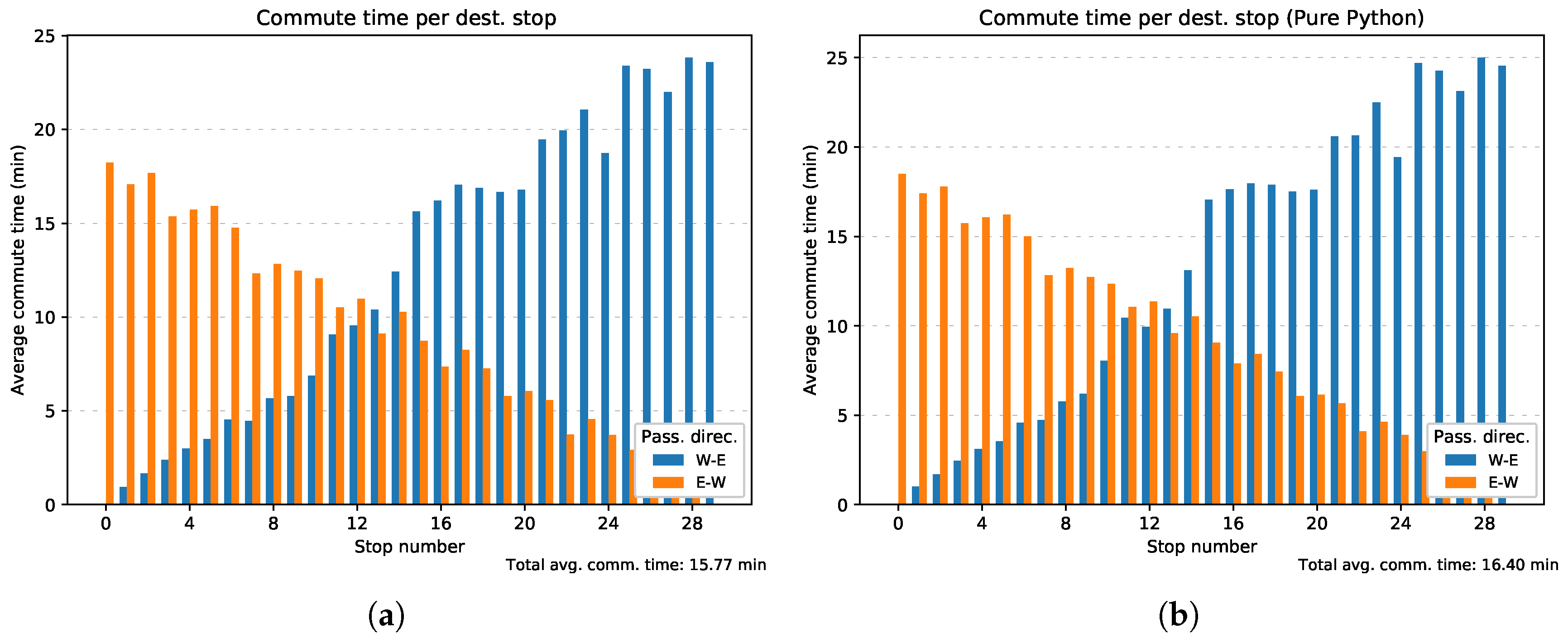
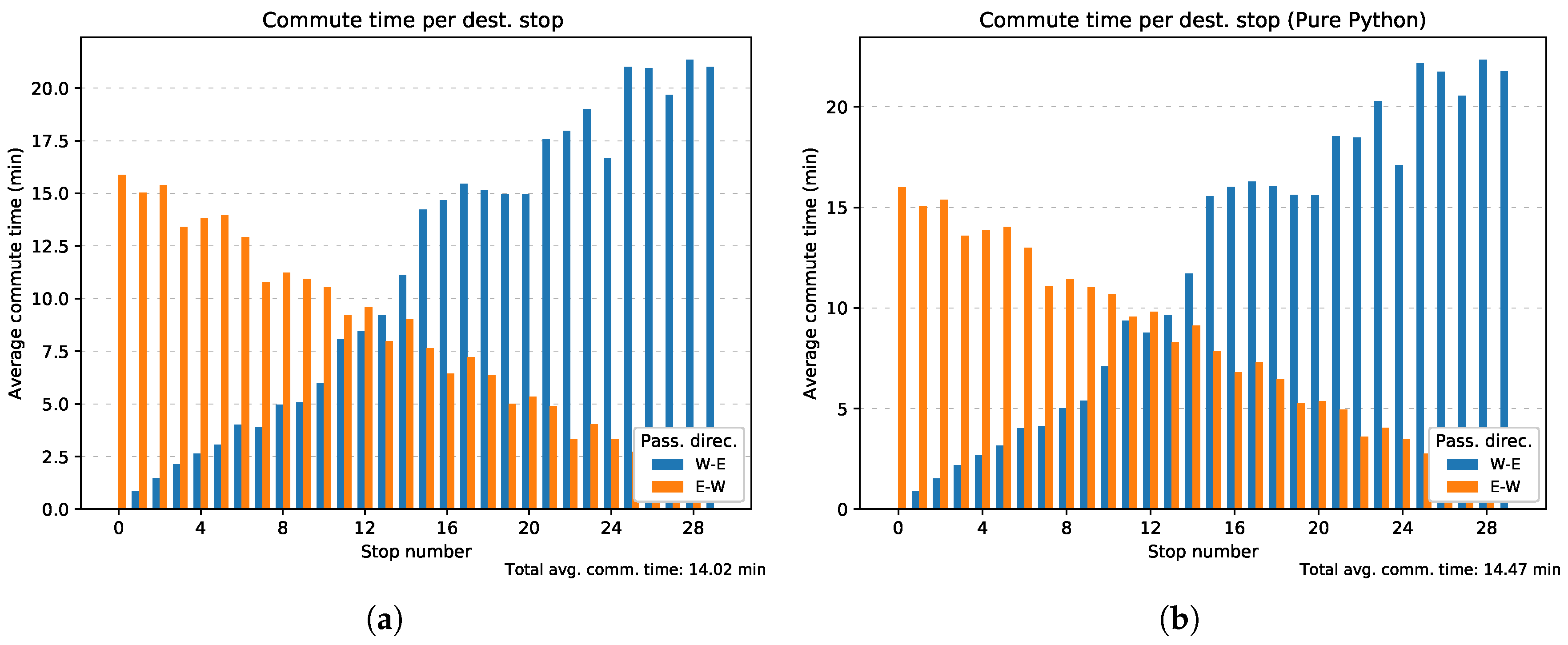
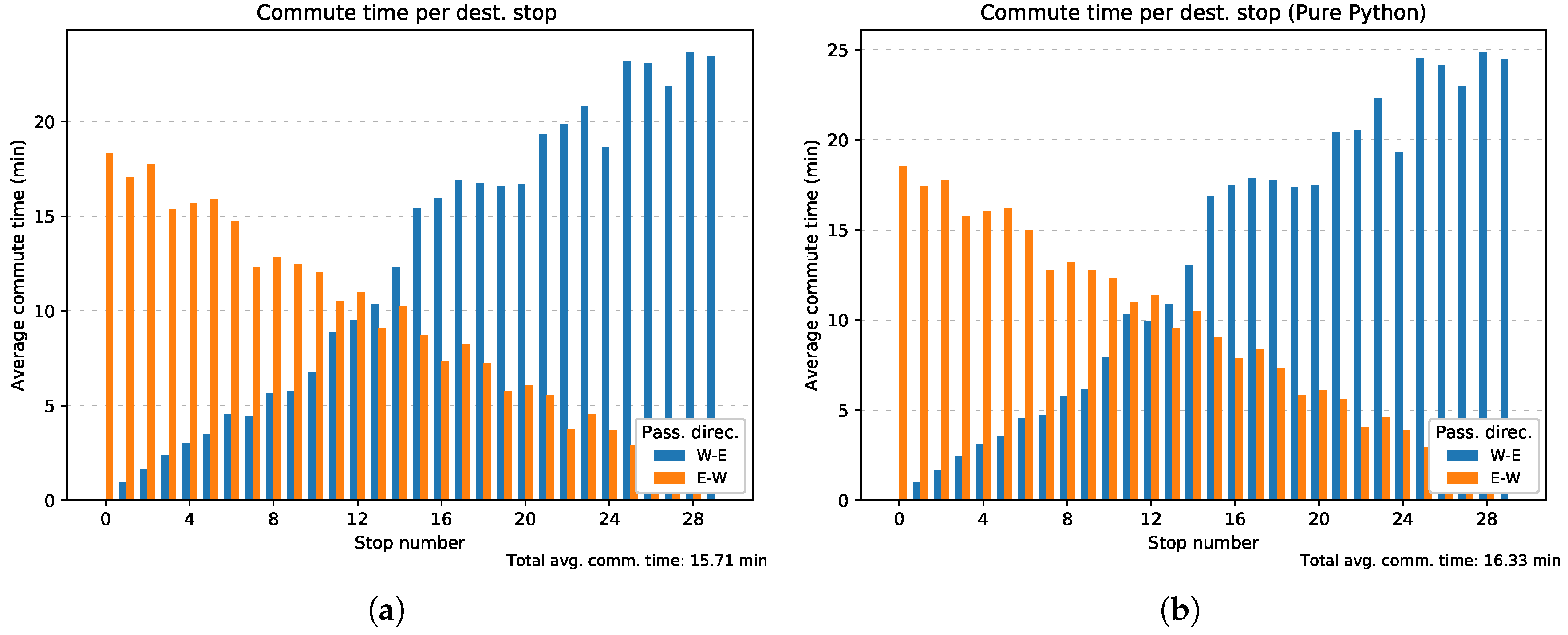
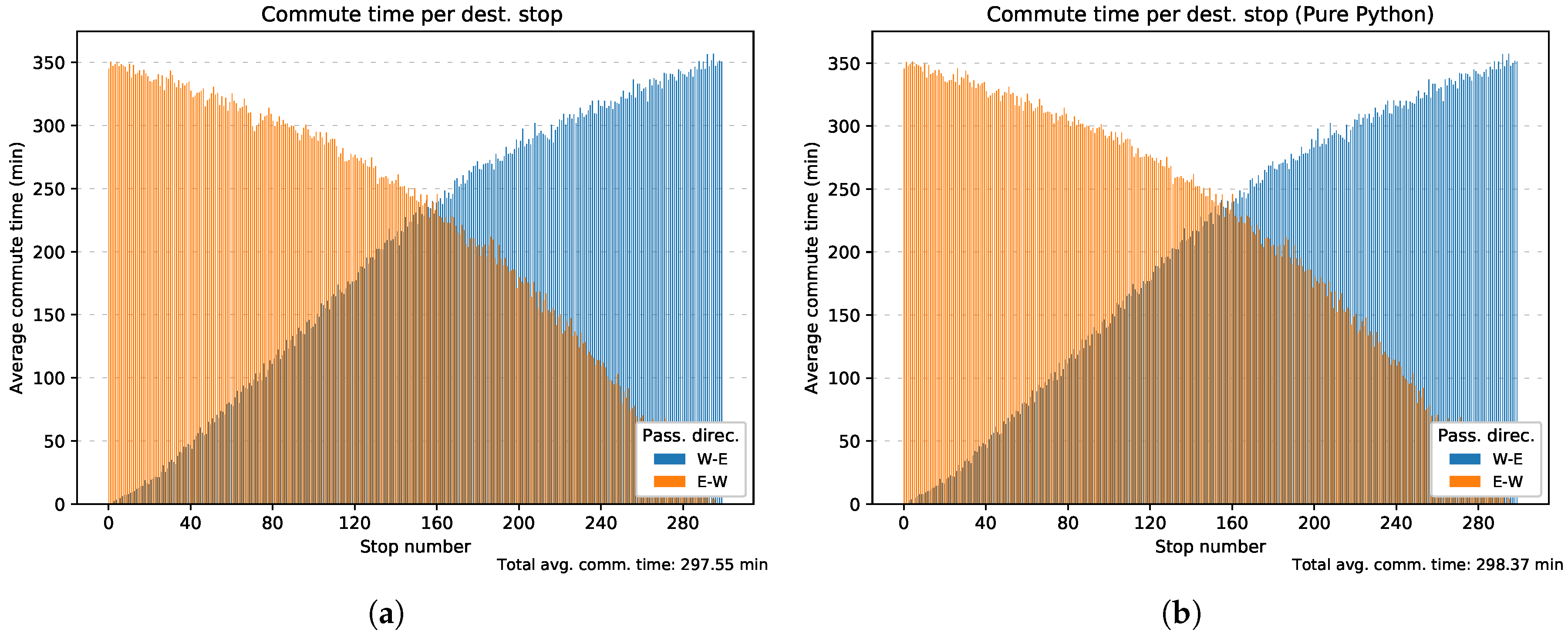
- commute_time_per_stop.eps: graphs the average commute time of the alighted passengers per destination stop and per travel direction. This graph is useful to see how the commute time is affected at a specific destination stop depending on traffic congestion on the road.
3.3.2. Performance Information
- performance_timeline.csv: contains the real-time simulation factor over time, with a sampling frequency of 100 s of the simulation. Furthermore, this file contains information related to CPU usage and CPU operation frequency over time.
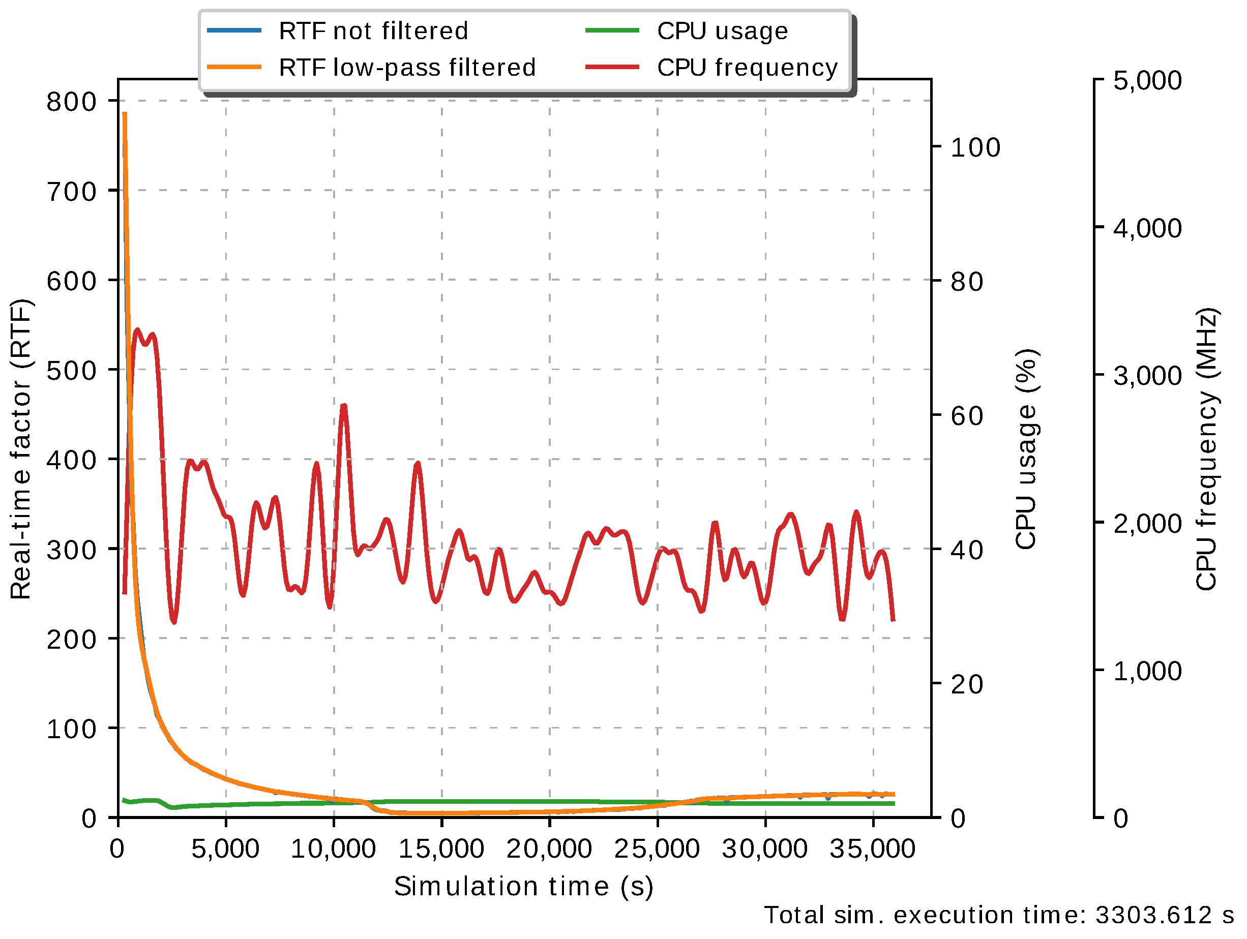
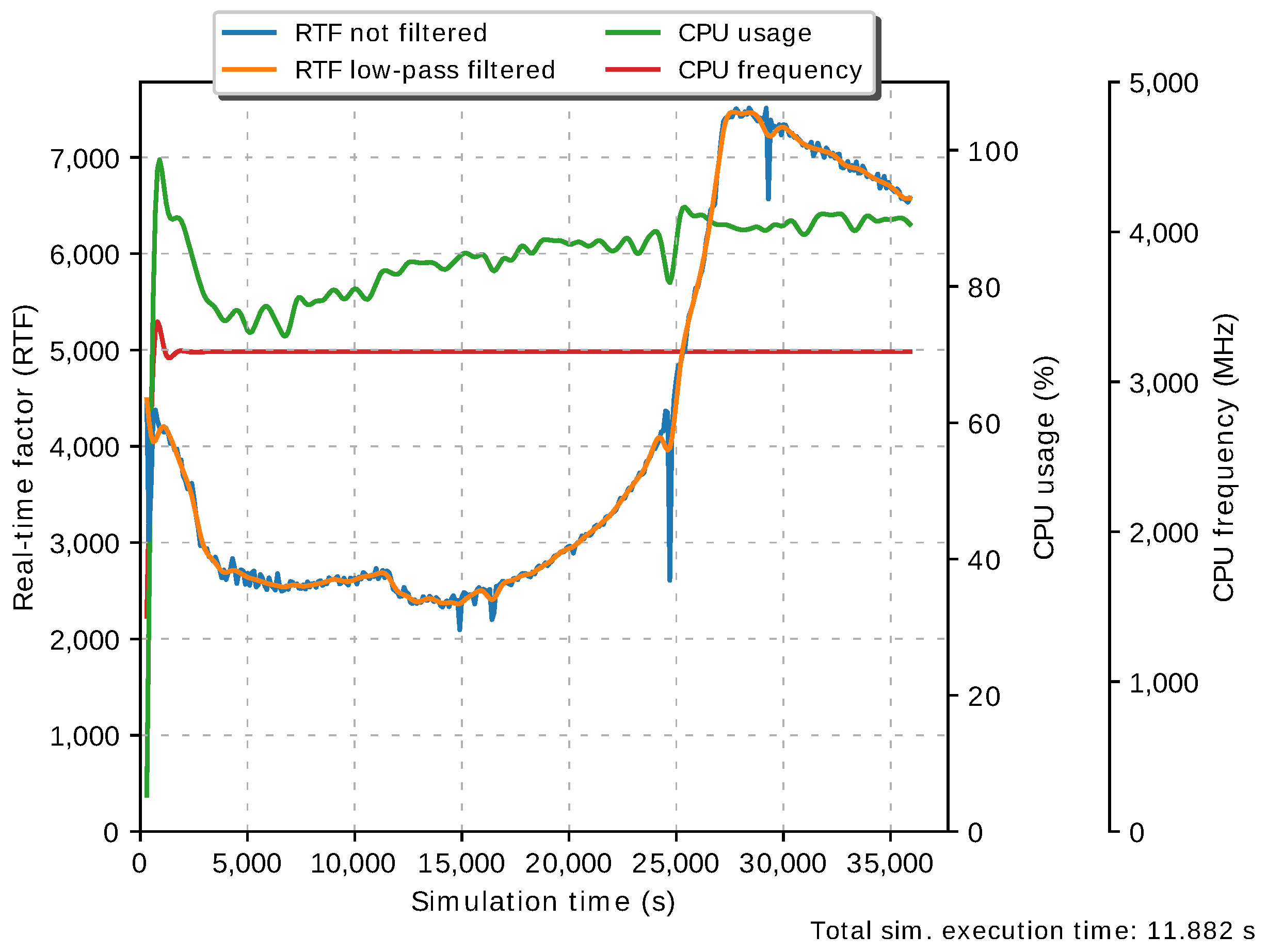
- performance_timeline.eps: graphs the real-time factor over time, the real-time factor low-pass filtered signal, the CPU usage, and the CPU operation frequency.
- simulation_brief.csv: contains all simulation configured parameters, total simulation outputs, and total performance indicators. In particular, as inputs, this file contains the buses’ average travel speed, bus max passengers, bus stopping time, end simulation time, ODM file, passenger total arrival time, routes’ file, and stop to bus windows’ distance. As outputs, we find here total alighted expected passengers, total alighted passengers, total alighted passenger percentage, total average commute time, total simulated buses, total simulated passengers, total routes, and total stops. Finally, for the total performance indicators, we include in this file the average CPU usage, average real-time factor, total simulation execution time, OpenCL device name and compute units used, and the limit of the max OpenCL compute units.
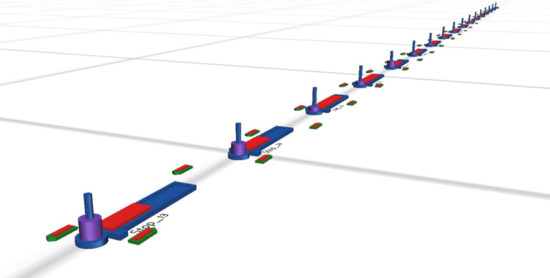
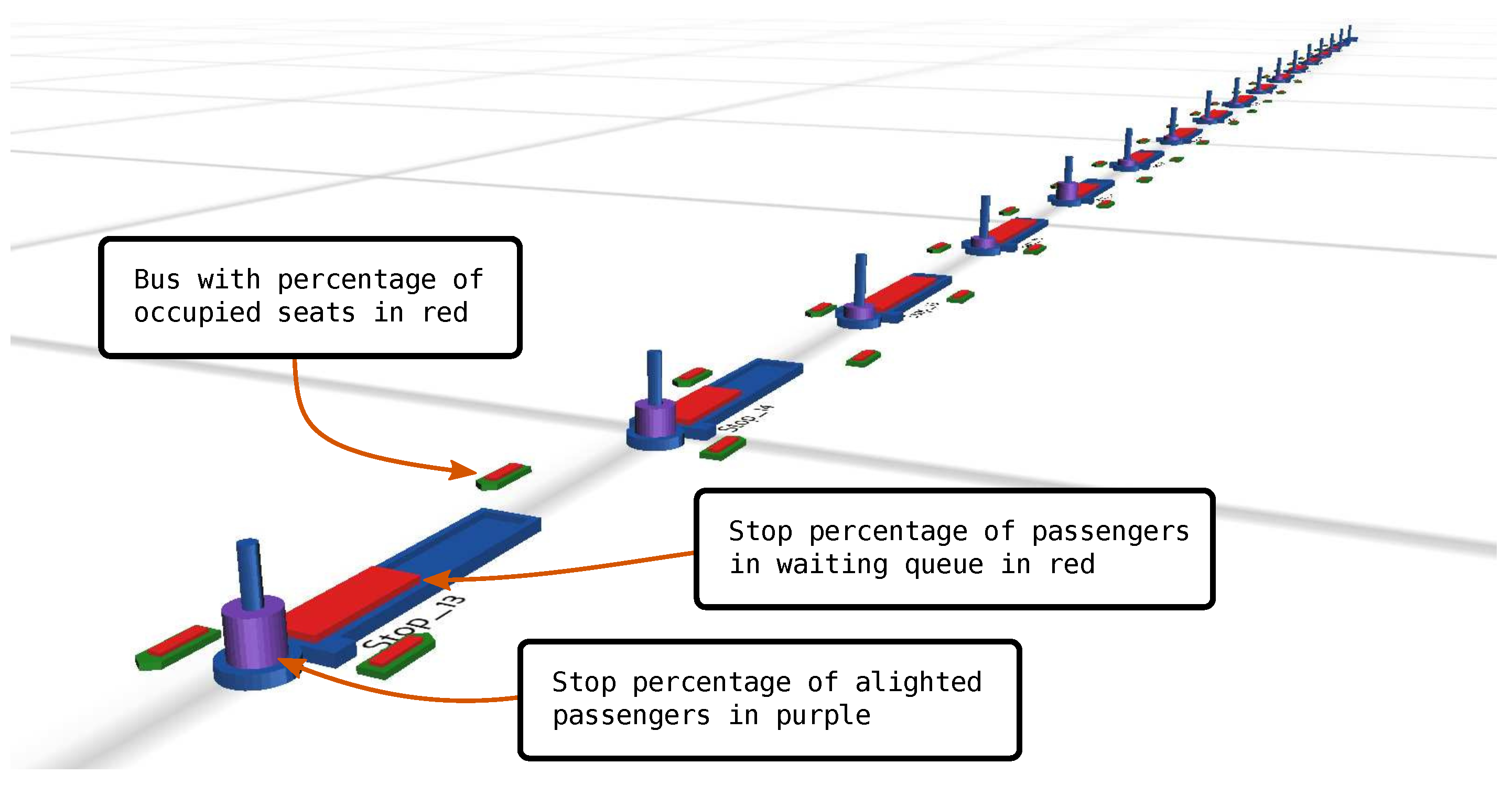
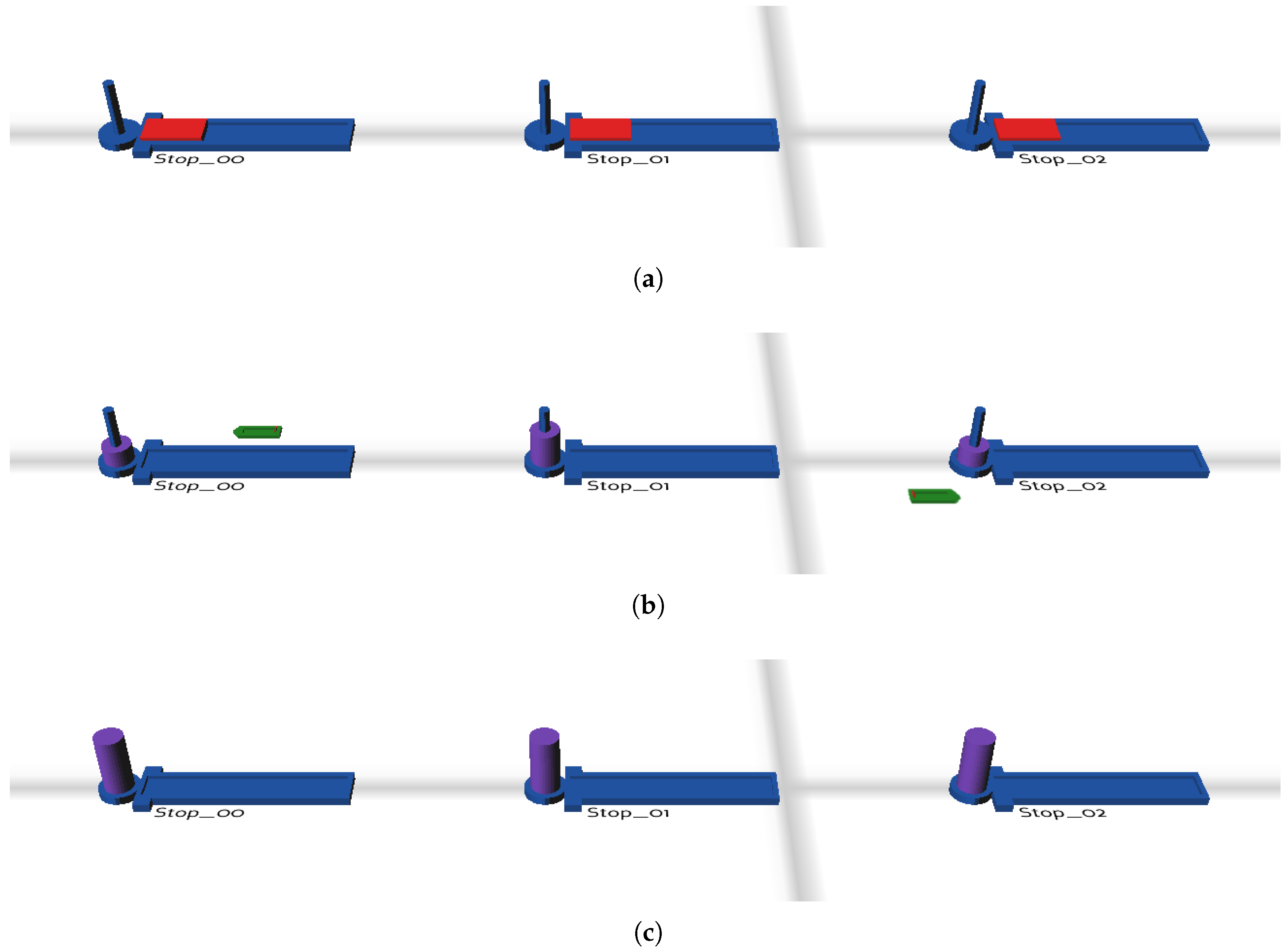
3.4. 3D System Visualization Output
3.5. Validation Simulator
4. Results
4.1. Validation Results
4.1.1. Scenario 1, 30 Stops and Two Routes at 54 km/h
4.1.2. Scenario 2, 30 Stops and Two Routes at 70 km/h
4.1.3. Scenario 3, 30 Stops and Four Routes at 54 km/h
4.1.4. Scenario 4, 300 Stops and Two Routes at 54 km/h
4.2. Performance
4.2.1. Pure Python Validation Simulator Performance
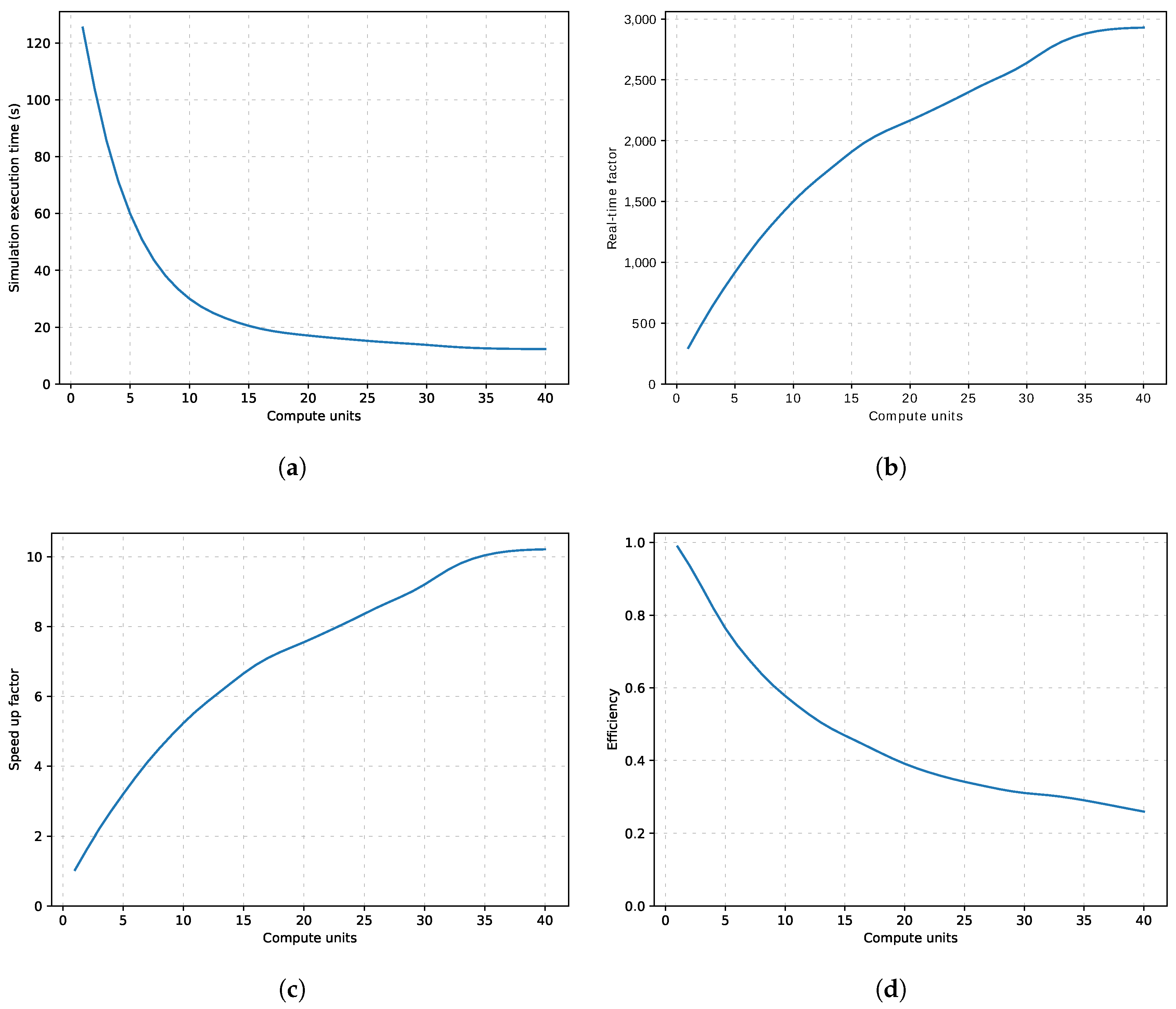
4.2.2. Masivo PSC Performance
5. Discussion
6. Conclusions
Author Contributions
Funding
Conflicts of Interest
References
- United Nations. World Urbanization Prospects; United Nations: New York, NY, USA, 2014; p. 32. [Google Scholar] [CrossRef]
- Ruiz-Rosero, J.; Ramirez-Gonzalez, G.; Williams, J.M.; Liu, H.; Khanna, R.; Pisharody, G. Internet of Things: A Scientometric Review. Symmetry 2017, 9, 301. [Google Scholar] [CrossRef]
- Ji, Y.; Mishalani, R.G.; McCord, M.R. Transit passenger origin–destination flow estimation: Efficiently combining onboard survey and large automatic passenger count datasets. Big Data in Transportation and Traffic Engineering. Transp. Res. Part C Emerg. Technol. 2015, 58, 178–192. [Google Scholar] [CrossRef]
- Budiawan, D.; Soenandi, I.A.; Marpaung, B. Optimilisasi Jumlah Armada Transjakarta di Koridor-8 Jurusan Harmoni-Lebak Bulus dengan Menggunakan Metode Goal Programming. Tek. Dan Ilmu Komput. 2014, 3, 128–137. [Google Scholar]
- Ergun, M.; Kesten, A.S. Alteration of bus routes in large-scale networks. Sci. Res. Essays 2011, 6, 5865–5882. [Google Scholar]
- Barceló, J. Models, Traffic Models, Simulation, and Traffic Simulation. In Fundamentals of Traffic Simulation; Springer: New York, NY, USA, 2010; pp. 1–62. [Google Scholar] [CrossRef]
- Loder, A.; Ambuehl, L.; Menendez, M.; Axhausen, K.W. Empirics of multi-modal traffic networks—Using the 3D macroscopic fundamental diagram. Transp. Res. Part C Emerg. Technol. 2017, 82, 88–101. [Google Scholar] [CrossRef]
- Oskarbski, J.; Birr, K.; Miszewski, M.; Zarski, K. Estimating the Average Speed of Public Transport Vehicles Based on Traffic Control System Data. In Proceedings of the 2015 International Conference on Models and Technologies for Intelligent Transportation Systems (MT-ITS), Budapest, Hungary, 3–5 June 2015. [Google Scholar]
- Truong, L.; Currie, G. Macroscopic road safety impacts of public transport: A case study of Melbourne, Australia. Accid. Anal. Prev. 2019, 132, 105270. [Google Scholar] [CrossRef]
- Drabicki, A.; Kucharski, R.; Cats, O.; Fonzone, A. Simulating the effects of real-time crowding information in public transport networks. In Proceedings of the 2017 5th IEEE International Conference on Models and Technologies for Intelligent Transportation Systems (MT-ITS), Naples, Italy, 26–28 June 2017. [Google Scholar]
- Johnsen, A.; Gundersen, E.; Liang, X.; Kaisar, E.; Scarlatos, P. Emergency evacuation methodologies utilizing public transit with meso-simulation. In Proceedings of the Simulation Interoperability Standards Organization—Spring Simulation Interoperability Workshop 2009, San Diego, CA, USA, 23–27 March 2009. [Google Scholar]
- Goh, Y.M.; Love, P.E.D. Methodological application of system dynamics for evaluating traffic safety policy. Saf. Sci. 2012, 50, 1594–1605. [Google Scholar] [CrossRef]
- Saprykin, A.; Chokani, N.; Abhari, R.S. GEMSim: A GPU-accelerated multi-modal mobility simulator for large-scale scenarios. Simul. Model. Pract. Theory 2019, 94, 199–214. [Google Scholar] [CrossRef]
- Fernandez, R. Modelling public transport stops by microscopic simulation. Transp. Res. Part C Emerg. Technol. 2010, 18, 856–868. [Google Scholar] [CrossRef]
- Fernandez, R.; Tyler, N. Effect of passenger-bus-traffic interactions on bus stop operations. Transp. Plan. Technol. 2005, 28, 273–292. [Google Scholar] [CrossRef]
- Yatskiv, I.; Pticina, I.; Savrasovs, M. Urban public transport system’s reliability estimation using microscopic simulation. Transp. Telecommun. 2012, 13, 219–228. [Google Scholar] [CrossRef]
- Yatskiv (Jackiva), I.; Pticina, I.; Romanovska, K. The Riga Public Transport Service Reliability Investigation Based on Traffic Flow Modelling. In Reliability and Statistics in Transportation and Communication; Springer: Berlin/Heidelberg, Germany, 2018; Volume 36. [Google Scholar] [CrossRef]
- Ahmed, B. Exploring new bus priority methods at isolated vehicle actuated junctions. Transp. Res. Procedia 2014, 14, 391–406. [Google Scholar] [CrossRef][Green Version]
- Arasan, V.T.; Vedagiri, P. Micro-simulation study of bus priority on roads carrying highly heterogeneous traffic. In Proceedings of the 22nd European Conference on Modeling and Simulation (ECMS), Nicosia, Cyprus, 3–6 June 2008. [Google Scholar]
- Thamizh, A.V.; Vedagiri, P. Microsimulation study of the effect of exclusive bus lanes on heterogeneous traffic flow. J. Urban Plan. Dev. 2010, 136, 50–58. [Google Scholar] [CrossRef]
- Chen, X.; Yu, L.; Zhu, L.; Guo, J.; Sun, M. Microscopic traffic simulation approach to the capacity impact analysis of weaving sections for the exclusive bus lanes on an urban expressway. J. Transp. Eng. 2010, 136, 895–902. [Google Scholar] [CrossRef]
- Chandrasekar, R.; Cheu, R.; Chin, H. Simulation evaluation of route-based control of bus operations. J. Transp. Eng. 2002, 128, 519–527. [Google Scholar] [CrossRef]
- Wang, J.; Chen, S.; He, Y.; Gao, L. Simulation of Transfer Organization of Urban Public Transportation Hubs. J. Transp. Syst. Eng. Inf. Technol. 2006, 6, 96–102. [Google Scholar] [CrossRef]
- Zargayouna, M.; Zeddini, B.; Scemama, G.; Othman, A. Agent-Based Simulator for Travelers Multimodal Mobility. In Advanced Methods and Technologies for Agent and Multi-Agent Systems; IOS Press: Amsterdam, The Netherlands, 2013; Volume 252. [Google Scholar] [CrossRef]
- Papageorgiou, G.; Damianou, P.; Pitsillides, A.; Aphamis, T.; Charalambous, D.; Ioannou, P. Modelling and Simulation of Transportation Systems: A Scenario Planning Approach. Automatika 2009, 50, 39. [Google Scholar]
- Ruiz-Rosero, J.; Ramirez-Gonzalez, G.; Viveros-Delgado, J. Software survey: ScientoPy, a scientometric tool for topics trend analysis in scientific publications. Scientometrics 2019, 121, 1165–1188. [Google Scholar] [CrossRef]
- Andrews, J.R.; Morrow, C.; Wood, R. Modeling the Role of Public Transportation in Sustaining Tuberculosis Transmission in South Africa. Am. J. Epidemiol. 2013, 177, 556–561. [Google Scholar] [CrossRef]
- Kadiyala, A.; Kumar, A. Multivariate Time Series Models for Prediction of Air Quality Inside a Public Transportation Bus Using Available Software. Environ. Prog. Sustain. Energy 2014, 33, 337–341. [Google Scholar] [CrossRef]
- Kadiyala, A.; Kumar, A. Vector time series models for prediction of air quality inside a public transportation bus using available software. Environ. Prog. Sustain. Energy 2014, 33, 1069–1073. [Google Scholar] [CrossRef]
- Kadiyala, A.; Kumar, A. Multivariate time series based back propagation neural network modeling of air quality inside a public transportation bus using available software. Environ. Prog. Sustain. Energy 2015, 34, 1259–1266. [Google Scholar] [CrossRef]
- Kadiyala, A.; Kumar, A. Univariate Time Series Based Back Propagation Neural Network Modeling of Air Quality Inside a Public Transportation Bus Using Available Software. Environ. Prog. Sustain. Energy 2015, 34, 319–323. [Google Scholar] [CrossRef]
- Kadiyala, A.; Kumar, A. Vector-time-series-based back propagation neural network modeling of air quality inside a public transportation bus using available software. Environ. Prog. Sustain. Energy 2016, 35, 7–13. [Google Scholar] [CrossRef]
- Kadiyala, A.; Kumar, A. Univariate time series based radial basis function neural network modeling of air quality inside a public transportation bus using available software. Environ. Prog. Sustain. Energy 2016, 35, 320–324. [Google Scholar] [CrossRef]
- Jappinen, S.; Toivonen, T.; Salonen, M. Modelling the potential effect of shared bicycles on public transport travel times in Greater Helsinki: An open data approach. Appl. Geogr. 2013, 43, 13–24. [Google Scholar] [CrossRef]
- Saghapour, T.; Moridpour, S.; Thompson, R.G. Modeling access to public transport in urban areas. J. Adv. Transp. 2016, 50, 1785–1801. [Google Scholar] [CrossRef]
- Nurlaela, S.; Curtis, C. Modeling household residential location choice and travel behavior and its relationship with public transport accessibility. In Proceedings of the 15th Meeting of the Euro-Working-Group-on-Transportation (EWGT), Cite Descartes, Paris, France, 10–13 September 2012; Elsevier Science BV: Amsterdam, The Netherlands, 2012; Volume 54, pp. 56–64. [Google Scholar] [CrossRef]
- Fuglsang, M.; Hansen, H.S.; Munier, B. Accessibility Analysis and Modelling in Public Transport Networks—A Raster Based Approach. In Proceedings of the 11th International Conference on Computational Science and Its Applications (ICCSA), Univ Cantabria, Santander, Spain, 20–23 June 2011; Springer: Berlin, Germany, 2011; Volume 6782, pp. 207–224. [Google Scholar]
- Schoebel, A. Line planning in public transportation: Models and methods. OR Spectr. 2012, 34, 491–510. [Google Scholar] [CrossRef]
- Schmidt, M.; Schoebel, A. The Complexity of Integrating Passenger Routing Decisions in Public Transportation Models. Networks 2015, 65, 228–243. [Google Scholar] [CrossRef]
- Schmidt, M.; SchoBel, A. The complexity of integrating routing decisions in public transportation models. In Proceedings of the 10th Workshop on Algorithmic Approaches for Transportation Modelling, Optimization, and Systems, ATMOS 2010, Liverpool, UK, 9–21 September 2010; Volume 14, pp. 156–169. [Google Scholar] [CrossRef]
- Abbas-Turki, A.; Grunder, O.; Elmoudni, A. Simulation and optimization of the public transportation connection system. In Proceedings of the 13th European Simulation Symposium, Marseille, France, 18–20 October 2001; pp. 435–439. [Google Scholar]
- Cats, O.; Gkioulou, Z. Modeling the impacts of public transport reliability and travel information on passengers’ waiting-time uncertainty. Euro J. Transp. Logist. 2017, 6, 247–270. [Google Scholar] [CrossRef]
- Hassannayebi, E.; Zegordi, S.H.; Yaghini, M.; Amin-Naseri, M.R. Timetable optimization models and methods for minimizing passenger waiting time at public transit terminals. Transp. Plan. Technol. 2017, 40, 278–304. [Google Scholar] [CrossRef]
- Kieu, L.M.; Cai, C. Stochastic collective model of public transport passenger arrival process. IET Intell. Transp. Syst. 2018, 12, 1027–1035. [Google Scholar] [CrossRef]
- Uspalyte-Vitkuniene, R.; Grigonis, V.; Paliulis, G. The Extent Of Influence of O-D Matrix on the Results of Public Transport Modeling. Transport 2012, 27, 165–170. [Google Scholar] [CrossRef]
- Kaiyuan, L.; Lifeng, L.; Feigang, T. A scheduling model and its implementation based on intelligent public transportation system. In Proceedings of the 2nd International Conference on Smart City and Systems Engineering (ICSCSE), Changsha, China, 11–12 November 2017; pp. 52–54. [Google Scholar] [CrossRef]
- Janoska, Z.; Dvorsky, J. P system based model of passenger flow in public transportation systems: A case study of Prague Metro. In Proceedings of the 13th Annual Workshop on Databases, Texts, Specifications and Objects (DATESO 2013), Pisek, Czech Republic, 17–19 April 2013; Volume 971, pp. 59–69. [Google Scholar]
- Yu, H.F.; Qin, Y.; Wang, Z.Y.; Wang, B.; Zhan, M.H. Research on urban mass transit network passenger flow simulation on the basis of multi-agent. In Proceedings of the International Conference on Information Technology and Computer Application Engineering (ITCAE), Hong Kong, China, 27–28 August 2013; CRC Press-Taylor & Francis Group: Boca Raton, FL, USA, 2014; pp. 225–229. [Google Scholar]
- Hadas, Y.; Ranjitkar, P. Modeling public-transit connectivity with spatial quality-of-transfer measurements. J. Transp. Geogr. 2012, 22, 137–147. [Google Scholar] [CrossRef]
- Ceder, A.; Chowdhury, S.; Taghipouran, N.; Olsen, J. Modelling public-transport users’ behaviour at connection point. Transp. Policy 2013, 27, 112–122. [Google Scholar] [CrossRef]
- He, R.; Li, Y.; Zhang, Z. Models and genetic algorithms for the optimal riding routes with transfer times limited in urban public transportation. In Proceedings of the 5th International Symposium on Operations Research and Its Applications, Tibet, China, 8–13 August 2005; Volume 5, pp. 340–348. [Google Scholar]
- Debinska, E.; Cichocinski, P. The application of multimodal network for the modeling of movement in public transport. In Proceedings of the 13th International Multidisciplinary Scientific Geoconference, SGEM 2013, Albena, Bulgaria, 16–22 June 2013; pp. 559–563. [Google Scholar]
- Rasmusseni, T.K.; Anderson, M.K.; Nielsen, O.A.; Prato, C.G. Timetable-based simulation method for choice set generation in large-scale public transport networks. Eur. J. Transp. Infrastruct. Res. 2016, 16, 467–489. [Google Scholar]
- Drabicki, A.; Kucharski, R.; Szarata, A. Modelling the public transport capacity constraints’ impact on passenger path choices in transit assignment models. Arch. Transp. 2017, 43, 7–28. [Google Scholar] [CrossRef]
- Fu, Z.; Yu, J.; Sarwat, M. Demonstrating geosparksim: A scalable microscopic road network traffic simulator based on Apache spark. In Proceedings of the 16th International Symposium on Spatial and Temporal Databases, Vienna, Austria, 19–21 August 2019; pp. 186–189. [Google Scholar] [CrossRef]
- Vu, V.A.; Tan, G. A Framework for Mesoscopic Traffic Simulation in GPU. IEEE Trans. Parallel Distrib. Syst. 2019, 30, 1691–1703. [Google Scholar] [CrossRef]
- Saprykin, A.; Chokani, N.; Abhari, R. Large-scale multi-agent mobility simulations on a GPU: Towards high performance and scalability. Procedia Comput. Sci. 2019, 151, 733–738. [Google Scholar] [CrossRef]
- Vu, V.; Tan, G. High-performance mesoscopic traffic simulation with GPU for large scale networks. In Proceedings of the 2017 IEEE/ACM 21st International Symposium on Distributed Simulation and Real Time Applications (DS-RT), Rome, Italy, 18–20 October 2017; Volume 2017, pp. 1–9. [Google Scholar] [CrossRef]
- Song, X.; Xie, Z.; Xu, Y.; Tan, G.; Tang, W.; Bi, J.; Li, X. Supporting real-world network-oriented mesoscopic traffic simulation on GPU. Simul. Model. Pract. Theory 2017, 74, 46–63. [Google Scholar] [CrossRef]
- Xu, Y.; Tan, G.; Li, X.; Song, X. Mesoscopic Traffic Simulation on CPU/GPU. In Proceedings of the SIGSIM-PADS’14: 2014 Acm Conference on Sigsim Principles of Advanced Discrete Simulation, Denver, CO, USA, 18–21 May 2014; Assoc Computing Machinery: New York, NY, USA, 2014. [Google Scholar]
- Xiao, J.; Andelfinger, P.; Eckhoff, D.; Cai, W.; Knoll, A. Exploring Execution Schemes for Agent-Based Traffic Simulation on Heterogeneous Hardware. In Proceedings of the 2018 IEEE/ACM 22nd International Symposium on Distributed Simulation and Real Time Applications (DS-RT), Madrid, Spain, 15–17 October 2018; pp. 243–252. [Google Scholar] [CrossRef]
- Janczykowski, M.; Turek, W.; Malawski, M.; Byrski, A. Large-scale urban traffic simulation with Scala and high-performance computing system. J. Comput. Sci. 2019, 35, 91–101. [Google Scholar] [CrossRef]
- Turek, W. Erlang-based desynchronized urban traffic simulation for high-performance computing systems. Future Gener. Comput. Syst. 2018, 79, 645–652. [Google Scholar] [CrossRef]
- Turek, W.; Siwik, L.; Byrski, A. Leveraging rapid simulation and analysis of large urban road systems on HPC. Transp. Res. Part C: Emerg. Technol. 2018, 87, 46–57. [Google Scholar] [CrossRef]
- Fu, Z.; Yu, J.; Sarwat, M. Building a large-scale microscopic road network traffic simulator in apache spark. In Proceedings of the 2019 20th IEEE International Conference on Mobile Data Management (MDM), Hong Kong, China, 10–13 June 2019; Voume 2019, pp. 320–328. [Google Scholar] [CrossRef]
- Public-Transport Noun—Definition, Pictures, Pronunciation and Usage Notes: Oxford Advanced Learner’s Dictionary. Available online: OxfordLearnersDictionaries.com (accessed on 1 December 2019).
- Desaulniers, G.; Hickman, M.D. Chapter 2 Public Transit. In Transportation. Handbooks in Operations Research and Management Science; Barnhart, C., Laporte, G., Eds.; Elsevier: Amsterdam, The Netherlands, 2007; Volume 14, pp. 69–127. [Google Scholar] [CrossRef]
- Barua, B.; Boberg, J.; Hsiao, S.; Zhang, X. Integrating Geographic Information Systems with Transit Survey Methodology. Transp. Res. Rec. 2001, 1753, 29–34. [Google Scholar] [CrossRef]
- Kuwahara, M.; Sullivan, E.C. Estimating origin-destination matrices from roadside survey data. Transp. Res. Part B Methodol. 1987, 21, 233–248. [Google Scholar] [CrossRef]
- Munizaga, M.A.; Palma, C. Estimation of a disaggregate multimodal public transport Origin–Destination matrix from passive smart card data from Santiago, Chile. Transp. Res. Part C Emerg. Technol. 2012, 24, 9–18. [Google Scholar] [CrossRef]
- Farzin, J.M. Constructing an Automated Bus Origin–Destination Matrix Using Farecard and Global Positioning System Data in São Paulo, Brazil. Transp. Res. Rec. 2008, 2072, 30–37. [Google Scholar] [CrossRef]
- White, J. Extracting origin destination information from mobile phone data. In Proceedings of the Eleventh International Conference on Road Transport Information and Control, London, UK, 19–21 March 2002; pp. 30–34. [Google Scholar]
- Fellendorf, M.; Vortisch, P. Validation of the microscopic traffic flow model VISSIM in different real-world situations. In Proceedings of the Transportation Research Board 80th Annual Meeting, Washington, DC, USA, 7–11 January 2001. [Google Scholar]
- Kotusevski, G.; Hawick, K. A Review of Traffic Simulation Software. Res. Lett. Inf. Math. Sci. 2009, 13, 1–19. [Google Scholar]
- Burghout, W.; Wahlstedt, J. Hybrid traffic simulation with adaptive signal control. Transp. Res. Rec. J. Transp. Res. Board 2015, 1999, 191–197. [Google Scholar] [CrossRef]
- Burghout, W. Mesoscopic Simulation Models For Short-Term Prediction; Royal Institute of Technology: Melbourne, Australia, 2005. [Google Scholar]
- Balakrishna, R.; Antoniou, C.; Ben-Akiva, M.; Koutsopoulos, H.; Wen, Y. Calibration of microscopic traffic simulation models: Methods and application. Transp. Res. Rec. J. Transp. Res. Board 2015, 1999, 198–207. [Google Scholar] [CrossRef]
- Bu, R. Simulación: Un Enfoque Práctico; Ingenieria Industrial; Publisher Editorial Limusa: Mexico City, Mexico, 1994. [Google Scholar]
- Yang, Q.; Koutsopoulos, H.; Ben-Akiva, M. Simulation laboratory for evaluating dynamic traffic management systems. Transp. Res. Rec. J. Transp. Res. Board 2000, 1710, 22–130. [Google Scholar] [CrossRef]
- Jayakrishnan, R.; Cortes, C.E.; Lavanya, R.; Pagès, L. Simulation of urban transportation networks with multiple vehicle classes and services: Classifications, functional requirements and general-purpose modeling schemes. In Proceedings of the TRB 2003 Annual Meeting, Washington, DC, USA, 12–16 January 2003. [Google Scholar]
- Bazzan, A.L.; Klügl, F. A review on agent-based technology for traffic and transportation. Knowl. Eng. Rev. 2014, 29, 375–403. [Google Scholar] [CrossRef]
- Buisson, C.; Lebacque, J.; Lesort, J. STRADA, a discretized macroscopic model of vehicular traffic flow in complex networks based on the Godunov scheme. In Proceedings of the CESA’96 IMACS Multiconference: Computational Engineering in Systems Applications, Lille, France, 9–12 July 1996; pp. 976–981. [Google Scholar]
- Haj-Salem, H.; Elloumi, N.; Mammar, S.; Papageorgiou, M.; Chrisoulakis, J.; Middelham, F. Metacor: A macroscopic modelling tool for urban corridor. In Towards An Intelligent Transport System, Proceedings of the First World Congress on Applications of Transport Telematics and Intelligent Vehicle-Highway Systems, Paris, France, 30 November–3 December 1994; TRB: Washington, DC, USA, 1994; Volume 3. [Google Scholar]
- PTV. VISUM 11.50 User Manual; PTV: Karlsruhe, Germany, 2011. [Google Scholar]
- Inro Software. The World’s Most Trusted Transportation Forecasting Software; Emme: Westmount, QC, Canada, 2015. [Google Scholar]
- Behrisch, M.; Bieker, L.; Erdmann, J.; Krajzewicz, D. SUMO–Simulation of Urban MObility. In Proceedings of the The Third International Conference on Advances in System Simulation (SIMUL 2011), Barcelona, Spain, 23–29 October 2011. [Google Scholar]
- AG, PTV Planug Trasport Verker. PTV Vissim 6 User Manual; PTV: Karlsruhe, Germany, 2013. [Google Scholar]
- Casas, J.; Ferrer, J.L.; Garcia, D.; Perarnau, J.; Torday, A. Traffic simulation with aimsun. In Fundamentals of Traffic Simulation; Springer: Berlin/Heidelberg, Germany, 2010; pp. 173–232. [Google Scholar]
- Maerivoet, S. Models in Aid of Traffic Management. In Proceedings of the Seminar slides for ‘Transportmodellen ter ondersteuning van het mobiliteits-en vervoersbeleid, Brussels, Belgium, 3 May 2004. [Google Scholar]
- Yang, H.; Cheng, W.; Xiao, H.C.; Pan, Y.W.; Zhang, D.M. Study of Traffic Flow Adjustment Methods to Congestion Area Based on TransModeler. Sci. Technol. Eng. 2011, 8, 022. [Google Scholar]
- Suping, L.F.C.X.C. Frequency optimization of bus rapid transit based on cost analysis. J. Southeast Univ. (Natural Sci. Ed.) 2009, 4, 038. [Google Scholar]
- Cortés, C.E.; Sáez, D.; Milla, F.; Núñez, A.; Riquelme, M. Hybrid predictive control for real-time optimization of public transport systems’ operations based on evolutionary multi-objective optimization. Transp. Res. Part C Emerg. Technol. 2010, 18, 757–769. [Google Scholar] [CrossRef]
- Kwan, R.S.K. Case studies of successful train crew scheduling optimisation. J. Sched. 2011, 14, 423–434. [Google Scholar] [CrossRef]
- Michael, R.G.; David, S.J. Computers and Intractability: A Guide to the Theory of NP-Completeness; WH Freeman & Co.: San Francisco, CA, USA, 1979. [Google Scholar]
- Lee, D.H.; Chandrasekar, P. A Framework for Parallel Traffic Simulation Using Multiple Instancing of a Simulation Program. J. Intell. Transp. Syst. 2002, 7, 279–294. [Google Scholar] [CrossRef]
- Nagel, K.; Rickert, M. Parallel implementation of the TRANSIMS micro-simulation. Parallel Comput. 2001, 27, 1611–1639. [Google Scholar] [CrossRef]
- Ruiz-Rosero, J.; Ramirez-Gonzalez, G.; Khanna, R. Field Programmable Gate Array Applications—A Scientometric Review. Computation 2019, 7, 63. [Google Scholar] [CrossRef]
- Hansson, A.; Mortveit, H.; Tripp, J.; Gokhale, M. Urban traffic simulation modeling for reconfigurable hardware. In Proceedings of the 3rd Industrial Simulation Conference 2005, Fraunhofer-IPK, Berlin, Germany, 9–11 June 2005; pp. 291–298. [Google Scholar]
- Wang, K.; Shen, Z. A GPU based trafficparallel simulation module of artificial transportation systems. In Proceedings of the 2012 IEEE International Conference on Service Operations and Logistics, and Informatics, SOLI 2012, Suzhou, China, 8–10 July 2012. [Google Scholar] [CrossRef]
- Potuzak, T. Distributed-Parallel Road Traffic Simulator for Clusters of Multi-core Computers. In Proceedings of the 2012 IEEE/ACM 16th International Symposium on Distributed Simulation and Real Time Applications (DS-RT), Dublin, Ireland, 25–27 October 2012. [Google Scholar] [CrossRef]
- Bruegmann, J.; Schreckenberg, M.; Luther, W. Real-time Traffic Information System Using Microscopic Traffic Simulation. In Proceedings of the 2013 8th Eurosim Congress on Modelling and Simulation (EUROSIM), Wales, UK, 10–13 September 2013. [Google Scholar] [CrossRef]
- Fernandes, R.; Vieira, F.; Ferreira, M. Parallel Microscopic Simulation of Metropolitan-scale Traffic. In Proceedings of the 46th Annual Simulation Symposium (ANSS 2013)—2013 Spring Simulation Multiconference (Springsim’13), San Diego, CA, USA, 7–10 April 2013; Volume 45. [Google Scholar]


| Variable Name | Symbol |
|---|---|
| Total number of stops | N |
| Origin-destination matrix | |
| value for stop i to j | |
| Stops max capacity | |
| Stops X position | |
| Stops Y position |
| Variable Name | Symbol |
|---|---|
| Total number of routes | R |
| Max buses per routes | |
| Routes frequency | |
| Max bus capacity | |
| Route stop table array |
| Variable Name | Symbol |
|---|---|
| Departed passengers from stop | |
| Alighted passengers at stop | |
| Average passengers commute time | |
| at alight stop n |
| Variable Name | Symbol |
|---|---|
| Total simulation time | |
| Total parallel simulation execution time | |
| Total sequential simulation execution time | |
| Real-time factor | |
| Speed-up factor | |
| Efficiency | |
| Number of processing threads | p |
| Stop_Number | Stop_Name | x_Pos | y_Pos | Max_Capacity | Stop_00 | Stop_01 | Stop_02 |
|---|---|---|---|---|---|---|---|
| 0 | Stop_00 | 400 | 1000 | 200 | 0 | 10 | 20 |
| 1 | Stop_01 | 800 | 1000 | 200 | 10 | 0 | 10 |
| 2 | Stop_02 | 1200 | 1000 | 200 | 20 | 10 | 0 |
| Number | Name | Freq. | Offset | Buses | Dir. | Notes | Stops_Table |
|---|---|---|---|---|---|---|---|
| 0 | Route_00 | 300 | 100 | 50 | W-E | all stops | Stop_00, Stop_01, Stop_02 |
| 1 | Route_01 | 300 | 100 | 50 | E-W | all stops | Stop_02, Stop_01, Stop_00 |
| 2 | Route_02 | 900 | 100 | 50 | W-E | express | Stop_00, Stop_02 |
| 3 | Route_03 | 900 | 100 | 50 | E-W | express | Stop_02, Stop_00 |
| Number | Name | Freq. | Offset | Buses | Dir. | Notes | Stops_Table |
|---|---|---|---|---|---|---|---|
| 0 | Route_00 | 900 | 950 | 50 | W-E | all stops | Stop_00, Stop_01, Stop_02 |
| 1 | Route_01 | 900 | 950 | 50 | E-W | all stops | Stop_02, Stop_01, Stop_00 |
| Condition | Value |
|---|---|
| Bus average transit speed (km/h) | 54 |
| Bus maximum passengers | 250 |
| Bus stopping time (s) | 20 |
| End simulation time (s) | 7200 |
| Passenger total arrival time (s) | 3600 |
| Total passengers | 38,721 |
| Total routes | 2 |
| Total stops | 30 |
| Condition | Value |
|---|---|
| Bus average transit speed (km/h) | 70 |
| Bus maximum passengers | 250 |
| Bus stopping time (s) | 20 |
| End simulation time (s) | 7200 |
| Passenger total arrival time (s) | 3600 |
| Total passengers | 38,721 |
| Total routes | 2 |
| Total stops | 30 |
| Condition | Value |
|---|---|
| Bus average transit speed (km/h) | 54 |
| Bus maximum passengers | 250 |
| Bus stopping time (s) | 20 |
| End simulation time (s) | 7200 |
| Passenger total arrival time (s) | 3600 |
| Total passengers | 38,721 |
| Total routes | 4 |
| Total stops | 30 |
| Condition | Value |
|---|---|
| Bus average transit speed (km/h) | 54 |
| Bus maximum passengers | 250 |
| Bus stopping time (s) | 20 |
| End simulation time (s) | 36,000 |
| Passenger total arrival time (s) | 3600 |
| Total passengers | 456,997 |
| Total routes | 2 |
| Total stops | 300 |
| Specification | Value |
|---|---|
| Type | Dedicated Server 4XL |
| CPU | Intel Xeon Gold 6210U |
| # of Cores | 20 |
| # of Threads | 40 |
| Processor Base Frequency | 2.50 GHz |
| Max Turbo Frequency | 3.90 GHz |
| Cache | 27.5 MB |
| RAM | 192 GB |
| HDD | 2 × 4000 GB Hardware RAID 1 |
| OS | Ubuntu 16.04 |
| Condition | Value |
|---|---|
| Bus average transit speed (km/h) | 54 |
| Bus maximum passengers | 250 |
| Bus stopping time (s) | 20 |
| End simulation time (s) | 36,000 |
| Passenger total arrival time (s) | 3600 |
| Total passengers | 456,997 |
| Total routes | 2 |
| Total buses | 2400 |
| Total stops | 300 |
| Performance Indicator | Value |
|---|---|
| Total simulation execution time (s) | 3303.612 |
| Average real-time factor | 32.76 |
| Average CPU usage (%) | 2.19 |
| Performance Indicator | Value |
|---|---|
| Total simulation execution time (s) | 11.882 |
| Average real-time factor | 3050.84 |
| Average CPU usage (%) | 84.21 |
| Document Title | Year | Parallel Architecture | Model Type | Simulation Core | Speedup Factor | Real-Time Factor | Simulation Complexity | Reference |
|---|---|---|---|---|---|---|---|---|
| Urban traffic simulation modeling for reconfigurable hardware | 2005 | FPGA | Microscopic | Road traffic | 4.50 | Not specified | 100,000 intersections | [98] |
| A GPU based traffic parallel simulation module of artificial transportation systems | 2012 | GPU | Microscopic | Road traffic | 105.00 | 102.00 | 1600 intersections and 5000 vehicles | [99] |
| Mesoscopic traffic simulation on CPU/GPU | 2014 | GPU | Mesoscopic | Road traffic | 11.20 | 2364.00 | 10,201 nodes and 100,000 vehicles | [60] |
| Supporting real-world network oriented mesoscopic traffic simulation on GPU | 2017 | GPU | Mesoscopic | Road traffic | 2.37 | 1897.00 | 4106 OD pairs, 100,000 vehicles | [59] |
| GEMSim: A GPU accelerated multi-modal mobility simulator for large scale scenarios | 2019 | GPU | Mesoscopic | Public transit system | Not specified | 1300.00 | 27,873 stops and 100,000 passengers | [13] |
| A framework for mesoscopic traffic simulation in GPU | 2019 | GPU | Mesoscopic | Road traffic | 5.00 | Not specified | 4103 OD pairs, 300,000 vehicles | [56] |
| Distributed-parallel road traffic simulator for clusters of multi-core computers | 2012 | Multi-core | Microscopic | Road traffic | 3.32 | 163.00 | 1024 Crossroads | [100] |
| Real-time traffic information system using microscopic traffic simulation | 2013 | Multi-core | Microscopic | Road traffic | Not specified | 60.00 | 1300 cross-sections and 120,000 vehicles | [101] |
| Parallel microscopic simulation of metropolitan scale traffic | 2013 | Multi-core | Microscopic | Road traffic | 16.00 | 0.86 | 145,665 roads, 4,349,130 vehicles, and 0.1 s step time | [102] |
| Masivo PSC | 2019 | Multi-core | Mesoscopic | Public transit system | 10.20/278 | 3000 | 300 stops, 2400 buses, and 456,997 passengers, | N/A |
© 2019 by the authors. Licensee MDPI, Basel, Switzerland. This article is an open access article distributed under the terms and conditions of the Creative Commons Attribution (CC BY) license (http://creativecommons.org/licenses/by/4.0/).
Share and Cite
Ruiz-Rosero, J.; Ramirez-Gonzalez, G.; Khanna, R. Masivo: Parallel Simulation Model Based on OpenCL for Massive Public Transportation Systems’ Routes. Electronics 2019, 8, 1501. https://doi.org/10.3390/electronics8121501
Ruiz-Rosero J, Ramirez-Gonzalez G, Khanna R. Masivo: Parallel Simulation Model Based on OpenCL for Massive Public Transportation Systems’ Routes. Electronics. 2019; 8(12):1501. https://doi.org/10.3390/electronics8121501
Chicago/Turabian StyleRuiz-Rosero, Juan, Gustavo Ramirez-Gonzalez, and Rahul Khanna. 2019. "Masivo: Parallel Simulation Model Based on OpenCL for Massive Public Transportation Systems’ Routes" Electronics 8, no. 12: 1501. https://doi.org/10.3390/electronics8121501
APA StyleRuiz-Rosero, J., Ramirez-Gonzalez, G., & Khanna, R. (2019). Masivo: Parallel Simulation Model Based on OpenCL for Massive Public Transportation Systems’ Routes. Electronics, 8(12), 1501. https://doi.org/10.3390/electronics8121501