Distributionally Robust Model of Energy and Reserve Dispatch Based on Kullback–Leibler Divergence

Abstract

This paper proposes a distance-based distributionally robust energy and reserve (DB-DRER) dispatch model via Kullback–Leibler (KL) divergence, considering the volatile of renewable energy generation. Firstly, a two-stage optimization model is formulated to minimize the expected total cost of energy and reserve (ER) dispatch. Then, KL divergence is adopted to establish the ambiguity set. Distinguished from conventional robust optimization methodology, the volatile output of renewable power generation is assumed to follow the unknown probability distribution that is restricted in the ambiguity set. DB-DRER aims at minimizing the expected total cost in the worst-case probability distributions of renewables. Combining with the designed empirical distribution function, the proposed DB-DRER model can be reformulated into a mixed integer nonlinear programming (MINLP) problem. Furthermore, using the generalized Benders decomposition, a decomposition method is proposed and sample average approximation (SAA) method is applied to solve this problem. Finally, simulation result of the proposed method is compared with those of stochastic optimization and conventional robust optimization methods on the 6-bus system and IEEE 118-bus system, which demonstrates the effectiveness and advantages of the method proposed.

1. Introduction

During the past decades, the issues of fossil fuel depletion and climate change are becoming more and more grievous. To cope with these questions, renewable energy such as wind energy generation and photovoltaic (PV) generation has been integrated into power systems in large scale [1,2]. However, renewable energy has the nature of being intermittent and unpredictable, which leads to changes in power system operation, such as unit commitment (UC) problems, economic dispatch (ED) problems, energy and reserve (ER) dispatch problems [3,4,5]. How to balance the load and generation has become more and more difficult and considerable.

How to solve optimization problems caused by uncertainties has become a research hotspot. In solving optimization problems, the most used traditional method to tackle data uncertainty is stochastic optimization (SO). Stochastic approximation [6] and sample average approximation (SAA) [7] are two typical solution methods for stochastic programming. In these studies [8,9,10,11,12,13], results demonstrate that stochastic optimization has a good performance under uncertainties. Generally, in stochastic optimization, the variabilities are assumed to follow a determined probability distribution. However, some reasons may cause managers to make incorrect decisions. For example, imperfect data may result in inaccurate probability distribution or difficultly capturing probability distribution of uncertain parameters.

Robust optimization (RO) is another widely used technique to address uncertainty variabilities [14]. In robust optimization, the value of objective function is obtained by only considering the worst-case when the uncertain parameters are within a given uncertainty set. There has been some research in [15,16,17], where the uncertainty set is usually constructed as an affine set. RO requires less information for modeling the uncertain parameters, but the solution is very conservative as it only considers the worst-case scenario that usually cannot actually occur.

During recent years, distributionally robust optimization (DRO) has been proposed, which is a useful method to overcome the deficiencies of SO and RO [18]. Compared to RO, the superiority of DRO is less conservative. And different from SOs requiring explicit distribution of variables, DRO just requires a series of obscure distributions. In a DRO model, usually the objective is to optimize a problem under the worst case of the distribution in a set (i.e., ambiguity set). A family of distributions constructs the ambiguity set of a DRO problem. How to construct the ambiguity set is the key to a DRO problem, and there are two main methods: namely, the moment-based DRO method and distance-based DRO method.

The moment-based DRO usually defines an ambiguity set by limiting the mean and covariance of the distribution to a given value. In the field of power systems, the moment-based DRO method has been applied to solve some problems. Reference [19] studied the economic dispatch problem of power systems under the distribution information of random variable as ambiguous, the ambiguity set was constructed as an ellipsoidal by using the mean and the covariance matrix, and conditional value-at-risk management is used to reformulate the proposed DRO model into a solvable convex optimization. Reference [20] presented a chance-constrained programming approach to deal with the distribution expansion planning problem under uncertain renewables and loads, and a DRO model was applied to solve the uncertainty variables. In [21], a chance constraint distributionally robust formulation based on an ambiguity set was considered and derived an approximate semi-definite programming (SDP) model. To solve energy-reserve-storage co-dispatch problem and facilitate the uncertain renewable energy, a DRO combined with the chance constraints model was proposed in [22], and the model could be transformed into a second-order programming problem to be solved. By considering the uncertain variables of renewable energy production and load consumption, [23] proposed a data-driven DRO model to deal with the optimal power flow problem. Based on available historical data, all possible probability distributions were assumed to have the same mean and covariance property to construct the ambiguity set.

The moment-based DRO method needs statistical information to construct the ambiguity set. In general, the data are not fully utilized because the distribution knowledge contains more information than moments. Motivated by the deficiency of the moment-based DRO method, reference [24,25,26,27,28,29,30,31,32,33,34] investigated the distance-based DRO method. Usually, in a distance-based DRO model, the ambiguity set is constructed by probability distribution. The most widely used probability distance functions include Kullback–Leibler divergence, Prokhorov metric, and the Wasserstein metric [25]. Among the three probability distance functions, the Wasserstein distance-based distributionally robust function has been carried out to solve problems in power system fields. By using an adjustable uncertainty set, [26] studied the energy and reserve scheduling problem by considering the wind power uncertainty, and a two-stage data-driven DRO model was proposed, the ambiguity was defined as Wasserstein balls which contains all the possible probability distributions. In [27], two-stage distributionally robust linear programs could be reformulated into different models by considering different ambiguity sets, such as under a 2-Wasserstein ball centered at a discrete distribution, the distributionally robust linear program can be seen as a copositive program problem. When the ambiguity set as a 1-Wasserstein ball, the two-stage DRO problem is equivalent to a tractable linear program problem. Reference [28] proposed a data-driven distributionally robust framework for unit commitment based on Wasserstein metric considering the wind power generation forecasting errors, and results showed that the proposed method could immunize the solutions against the worst-case distribution in the ambiguity set. By constructing a data-driven ambiguity set of candidate distributions based on the Wasserstein metric, a novel data-driven Wasserstein DRO model for hedging against uncertainty in the optimal network design was proposed in [29]. To manage the risk from uncertain wind power forecasted errors, [30] proposed a Wasserstein metric-based distributionally robust approximate framework for the unit commitment problem. Different from the mature application of the Wasserstein metric, the application of Kullback–Leibler divergence needs further study. Under the volatile of wind power generation, [31] proposed a distance-based distributionally robust UC model via KL divergence. The objective function minimized the expected generation cost under the worst-case wind power generation distribution, and KL divergence was used to measure the distance between two distributions and to construct the ambiguity set. To shave the peak, reference [32] described a DRO model to schedule the heat pump day-ahead operation, KL divergence was applied to construct the ambiguity set of the DRO model by using a nominal distribution. Thus, the model could be transformed into a tractable deterministic model. In [33,34], the Kullback–Leibler divergence method was further studied in-depth in other scopes.

Motivated by the idea of using the available data to design appropriate uncertainty sets, in this paper, the distance-based DRO is applied to solve the ER dispatch problem under renewable energy generation uncertainty. The ambiguity set in this proposed model is constructed via KL divergence. The main contributions of the present paper are summarized as follows:

(1) A two-stage optimization model is established for the joint ER dispatch problem. In the first-stage problem (i.e., day-ahead dispatch), the objective function aims at minimizing generation and reserve cost under assuming the true output of renewable resource is known. The second-stage is the re-dispatch stage, which takes the real output of renewable resource into account.

(2) To utilize the known historical data, the ambiguity set is constructed by KL divergence theory, and the distance-based DRO model is established. The proposed model can be transformed into a mixed integer nonlinear programming (MINLP) problem. Based on the generalized Benders decomposition, a decomposition method and SAA are applied to solve the problem.

(3) The numerical test shows that the proposed approach is less conservative for decision making under the uncertainty of renewable resource output than the conventional RO model. In addition, the scale of the historical data is very critical for this method; the larger the scale is, the exacter the ambiguity set is and the less conservative the result is.

The rest of the paper is organized as follows. In Section 2, a two-stage model is established and KL divergence theory is introduced. The construction of the ambiguity set and model reformulation are described in Section 3. The solution method is given in detail in Section 4. Numerical results are simulated and discussed in Section 5. Finally, Section 6 summarizes the main conclusions and contributions of this study, and prospects are made.

2. Mathematical Formulation

2.1. Energy and Reserve Dispatch Model

Assuming that the projection of renewable energy resource outcome is determined, then the mathematical model of the first-stage problem can be presented which minimizes the total production cost subject to the operating constrains with respect to the renewable energy output forecast [35]:

$$\min {\displaystyle \sum _{i=1}^{N_G}(c_i^g{z}_i^g+a_i{p}_i{}^2+b_i{p}_i+c_i}+c_i^{r,up}{r}_i^{up}+c_i^{r,dw}{r}_i^{dw}),$$

(1)

$$s.t.p_i^l\le p_i-r_i^{dw},p_i+r_i^{up}\le p_i^u,$$

(2)

$${\displaystyle \sum _{i=1}^{N_G}{p}_i}+{\displaystyle \sum _{j=1}^{N_W}{\omega }_j^f}={\displaystyle \sum _{q=1}^{N_Q}{p}_q},$$

(3)

$$-{\overline{F}}_l\le f_{Nl}\left({\displaystyle \sum _{i=1}^{N_G}{p}_i}+{\displaystyle \sum _{j=1}^{N_W}{\omega }_j^f}-{\displaystyle \sum _{q=1}^{N_Q}{p}_q}\right)\le {\overline{F}}_l,$$

(4)

$$0\le r_i^{up}\le R_i^{up}\mathsf{\Delta }t,0\le r_i^{dw}\le R_i^{dw}\mathsf{\Delta }t,$$

(5)

$$z_i^g\in \{0,1\}.$$

(6)

In the first-stage mathematical model, objective (1) is the total production cost, including start-up cost, the generation cost, and the spinning reserve cost. Constraint (2) is the generation capacity limitation considering the spinning reserve. Constraint (3) is the power balance condition with respect to the renewable energy generation forecast. Constraint (4) is the power flow restriction of transmission lines with respect to the renewable energy generation forecast. Constraint (5) depicts that the spinning reserve capacity cannot exceed the ramping limit in the dispatch interval of the generator. Constraint (6) denotes the start-up variable of units.

The second-stage problem is formulated as:

$$\min {\displaystyle \sum _{i=1}^{N_G}\left(c_i^{g,up}{p}_i^{up}+c_i^{g,dw}{p}_i^{dw}\right)}+{\displaystyle \sum _{j=1}^{N_W}\left(c_j{\omega }_j^c\right)}+{\displaystyle \sum _{q=1}^{N_Q}\left(c_q{p}_q^l\right)},$$

(7)

$$s.t.{\displaystyle \sum _{q=1}^{N_Q}\left(p_q-p_q^l\right)}={\displaystyle \sum _{j=1}^{N_W}\left({\omega }_j^f+{\mathit{\xi }}_j-{\omega }_j^c\right)}+{\displaystyle \sum _{i=1}^{N_G}\left(p_i+p_i^{up}-p_i^{dw}\right)},$$

(8)

$$-{\overline{F}}_l\le f_{Nl}\left[{\displaystyle \sum _{i=1}^{N_G}\left(p_i+p_i^{up}-p_i^{dw}\right)}+{\displaystyle \sum _{j=1}^{N_W}\left({\omega }_j^f+{\mathit{\xi }}_j-{\omega }_j^c\right)}-{\displaystyle \sum _{q=1}^{N_Q}\left(p_q-p_q^l\right)}\right]\le {\overline{F}}_l,$$

(9)

$$0\le p_i^{up}\le r_i^{up},0\le p_i^{dw}\le r_i^{dw},$$

(10)

$$0\le {\omega }_j^c\le {\omega }_j^g,0\le p_q^l\le p_q,$$

(11)

$${\omega }_j^f={\omega }_j^g-{\mathit{\xi }}_j.$$

(12)

Objective (7) minimizes the cost of corrective actions when the actual power output of renewable energy is considered, including the generator re-dispatch cost, the renewable energy power spillage cost, and the load shedding cost. Constraint (8) is the power balance condition. Constraint (9) is the security limitation of transmission lines. Constraint (10) sets that the real-time re-dispatch capacity of generators cannot exceed its spinning reserve capacity preserved in the first-stage. Constraints (11) stipulates the bounds of renewable energy power curtailment and load shedding. The relationship of actual renewable energy power output and prediction renewable energy power output is expressed by constraint (12).

Thus, a two-stage optimization model according to the above analysis is obtained. To simplify the notations, the problem can be abstracted into a concise model as follows:

$$\min {\mathit{c}}^T\mathit{x}+Q\left(\mathit{x},\mathit{\xi }\right),$$

(13)

$$s.t.\mathit{A}\mathit{x}-\mathit{b}\le 0,$$

(14)

$$z_i^g\in \{0,1\},$$

(15)

where $\mathit{x}\in \mathit{X}=\left\{\mathit{x}\right|\mathit{A}\mathit{x}\le \mathit{b}\}$, (14) represents (2)–(5). The symbol $Q\left(x,\mathit{\xi }\right)$ is the optimal value of the second-stage problem:

$$\begin{array}{l}Q\left(\mathit{x},\mathit{\xi }\right)=\min {\mathit{q}}^T\mathit{y}\\ s.t.\mathit{T}\mathit{y}+\mathit{W}\mathit{x}\le \mathit{d}-\mathit{R}\mathit{\xi }\\ \mathit{x}\ge 0,\mathit{y}\ge 0\\ z_i^g\in \{0,1\}\end{array}$$

(16)

Matrices T, W, R, and vector d represent to the coefficients in constraints (8)–(12), the decision variables $\mathit{x}=\left\{p_i,r_i^{up},r_i^{dw}\right\}$ and $\mathit{y}=\left\{p_i^{up},p_i^{dw},w_j^c,p_q^l\right\}$ are in the first-stage and the second-stage, respectively. The forecast errors of variable renewable energy power is represented by vector $\mathit{\xi }$.

2.2. DRO Model Based on KL-Divergence

To construct a distance-based DRO model ambiguity set, available historical data are essential and used rational. Statistical distance functions, such as the Prokhorov metric, the Wasserstein metric, and the KL divergence are applied to address data analysis, which have some common properties and can co-transfer in some situations [15]. KL divergence originated from statistics and the information theory. The performance of KL divergence in measuring the distance between two probability distributions makes it be widely used. Different from the Prokhorov metric and the Wasserstein metric, the KL divergence has some obvious advantages. Firstly, KL divergence is a widely accepted measure of distances between distributions. Secondly, its tractability in solving DRO problems by reformulating the problem into a tractable problem can be solved by optimization tools. Furthermore, the available data through the KL divergence method can be fully used.

Mathematically, the KL divergence expression is generally defined as:

$$D_{KL}\left(P\parallel P_0\right)={\displaystyle {\int }_{\mathsf{\Omega }}P\left(\theta \right)}\log \frac{P\left(\theta \right)}{P_0\left(\theta \right)}d\theta ,$$

(17)

where P, P₀ are distribution functions in measure space Ω.

Many scholars have studied the DRO based on KL divergence [31,32,33,34], and they put forward some reformulation methods in the research. In these studies, KL divergence has been used to solve problems such as unit commitment, and showed its advantages.

According to the theory of KL divergence, and considering the ambiguous probability distributions, the distance-based distributionally robust energy and reserve (DB-DRER) model of (13) is proposed as follows:

$$\begin{array}{l}\min {\mathit{c}}^T\mathit{x}+\underset{P\in \mathcal{D}}{\max }{\mathbb{E}}_P\left[Q\left(\mathit{x},\mathit{\xi }\right)\right]\\ s.t.\mathit{A}\mathit{x}-\mathit{b}\le 0\\ \mathit{T}\mathit{y}+\mathit{W}\mathit{x}\le \mathit{d}-\mathit{R}\mathit{\xi }\\ \mathit{x}\ge 0,\mathit{y}\ge 0\\ z_i^g\in \{0,1\}\end{array}$$

(18)

where ${\mathbb{E}}_P\left[Q\left(\mathit{x},\mathit{\xi }\right)\right]$ denotes the expected value with respect to a distribution P of random variables $\mathit{\xi }$.

3. Reformulation of Optimization Model

In Section 3.1, we construct the ambiguity set by introducing KL divergence method, and a distributionally robust counterpart for the two-stage ER dispatch model (i.e., DB-DRER) is proposed. Then in Section 3.2, we reformulate the DB-DRER into a MINLP problem.

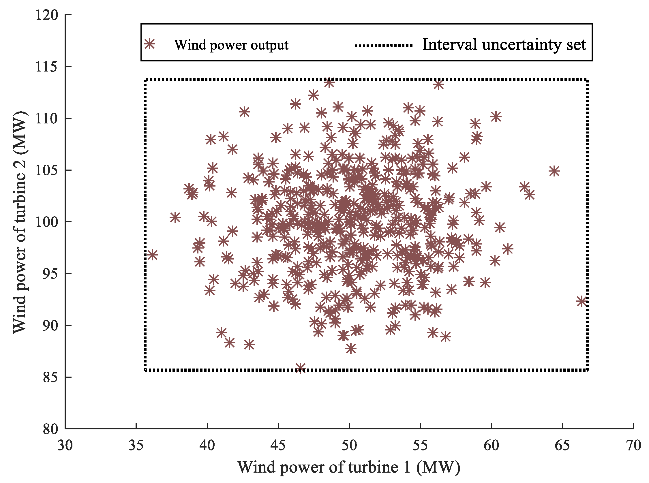
3.1. Ambiguity Set Construction

The ambiguity set affects the accuracy and conservatism of the dispatch planning. The structure of the ambiguity set has a large influence to the performance and tractability of the above problem. The underlying true probability distribution should be contained in a desirable ambiguity set. The desirable ambiguity set allows the reformulation of the DRO problem (18) into a tractable problem. Generally, the method of constructing the ambiguity set by the KL divergence can be expressed by:

$$\mathcal{D}:=\{P\in \mathcal{D}|D_{KL}\left(P\parallel P_0\right)\le \eta \},$$

(19)

where P₀ is the nominal distribution, which can be obtained by fitting historical data. η is the divergence tolerance, and it can control the size of the ambiguity set. The conservative of the DB-DRER model can be adjusted by setting different value of η.

In [36], some approaches are presented to construct uncertainty set. The most basic approach to construct an ambiguity set is to define a confidence interval for uncertainty variable, (e.g., 95% can be set as the confidence level value), but it is too simple to describe the correlation between variables and has strong conservation. Even though, this idea can be adopted to construct the ambiguity set in a similar method through determine the confidence level. Then:

$$\mathcal{D}:=\{P\in \mathcal{D}|D_{KL}\left(P\parallel P_0\right)\le {\eta }_{\alpha }\},$$

(20)

where α is confidence level, and ${\eta }_{\alpha }$ denotes the divergence tolerance. Formula (20) describes that the true distribution is within $\mathcal{D}$ with α confidence level.

To construct the ambiguity set, the key is to determine the value of nominal distribution P₀. In [37], there are many methods to obtain P₀, like parametric estimation method such as point estimation, interval estimation. However, they all assume the uncertainty variable follows a predefined distribution, which is usually unrealistic. On the contrary, non-parametric estimates do not require hypothetical distributions. To take advantage of nonparametric estimation, the nonparametric estimation method is adopted to construct the ambiguity set. Kernel density estimation is a widely used method in nonparametric estimation. In [38], Kernel density estimation is applied to construct an ellipsoidal uncertainty set and shows well performance. But the disadvantage is that the influence of boundary points should be considered in Kernel density estimation.

Reference [37] provides a way of thinking for us to use the nonparametric estimation method. Assuming that the historical relative predicted errors could be obtained, the Monte Carlo method is used to generate the scenarios [39]. $\left\{{\rho }_1,{\rho }_2,\cdots ,{\rho }_s\right\}$ are the probabilities represent variable $\left\{{\mathit{\xi }}_1,{\mathit{\xi }}_2,\cdots ,{\mathit{\xi }}_s\right\}$. Then, an empirical distribution is designed and can be expressed by:

$${\rho }_s=\frac{N_s}{N},s=1,2,\cdots ,\mathcal{S},$$

(21)

$\mathrm{where}\mathcal{S}$ denotes the total number of scenarios, ${\rho }_s$ is the nominal distribution probability of scenario s, Ns is the number of observations of scenarios, and follows (22):

$${\displaystyle \sum _{s=1}^{\mathcal{S}}{N}_s}=N.$$

(22)

3.2. RDB-DRER Model

In this section, KL divergence is used to reformulate problem (18). The objective function in (18) minimizes the total cost in the worst-case probability distribution and it cannot be solved directly by the existing solver. For convenience, to elaborate the process of reformulating the model, only the inner maximization section of objective function in (18) is given as follows:

$$\underset{P\in \mathcal{D}}{\max }{\mathbb{E}}_P\left[Q\left(\mathit{x},\mathit{\xi }\right)\right].$$

(23)

Formula (23) is the expected cost with respect to the worst-case probability distribution. $Q_s$ is used to represent $Q\left(\mathit{x},\mathit{\xi }\right)$, according to the analysis in the above Section 3.1, when P is discrete in (23), the special case of (23) can be expressed as follows:

$$\begin{array}{l}\underset{P\in \mathcal{D}}{\max }{\mathbb{E}}_P\left[Q\left(\mathit{x},\mathit{\xi }\right)\right]=\underset{s=1,2,\cdots \mathcal{S}}{\sup }{\displaystyle \sum _{s=1}^{\mathcal{S}}{\rho }_s^P{Q}_s}\\ s.t.\hspace{1em}\hspace{1em}{\displaystyle \sum _{s=1}^{\mathcal{S}}{\rho }_s^P}\log \left(\frac{{\rho }_s^P}{{\rho }_s}\right)\le \eta \\ \forall s=1,2,\cdots ,\mathcal{S}\end{array}$$

(24)

Based on strong duality theory, for η ≥ 0, the dual function of objective function in (24) can be transformed into:

$$\inf \lambda \eta +\nu +{\displaystyle \sum _{s=1}^{\mathcal{S}}\underset{{\rho }_s^P\ge 0}{\sup }{\rho }_s^P\left(Q_s-\nu -\lambda \log \frac{{\rho }_s^P}{{\rho }_s}\right)},$$

(25)

where $\lambda$ and $\nu$ are the new dual variables and:

$${\displaystyle \sum _{s=1}^{\mathcal{S}}{\rho }_s^P}=1.$$

(26)

Define $\frac{{\rho }_s^P}{{\rho }_s}=u$, then:

$$\inf \lambda \eta +\nu +{\displaystyle \sum _{s=1}^{\mathcal{S}}{\rho }_s\underset{u\ge 0}{\sup }u\left(Q_s-\nu -\lambda \log u\right)}.$$

(27)

According to reference [40], (27) is equivalent to the following problem:

$$\inf \lambda \eta +\nu +\lambda {\displaystyle \sum _{s=1}^{\mathcal{S}}{\rho }_s{e}^{(Q_s-\nu -\lambda )/\lambda }},$$

(28)

where ${\nu }^{*}$ is the optimal value of $\nu$, and it satisfies:

$${\displaystyle \sum _{s=1}^{\mathcal{S}}{\rho }_s{e}^{(Q_s-{\nu }^{*}-\lambda )/\lambda }=1},$$

(29)

$$v^{*}=\lambda \log {\displaystyle \sum _{s=1}^{\mathcal{S}}{\rho }_s}{e}^{Q_s/\lambda }-\lambda .$$

(30)

Substituting (29) and (30) into (28) can obtain (31):

$$\underset{\lambda \ge 0}{\min }\lambda \log {\displaystyle \sum _{s=1}^S{\rho }_s{e}^{Q_s/\lambda }}+\lambda \eta .$$

(31)

Then, (31) is equivalent to (32):

$$\underset{\lambda \ge 0}{\min }\lambda \log {\mathbb{E}}_{P_0}\left[e^{Q\left(\mathit{x},\mathit{\xi }\right)/\lambda }\right]+\lambda \eta .$$

(32)

(32) is a one-layer optimization problem and it has been discussed in [40]. Then, the problem (18) can be reformulate as:

$$\begin{array}{l}\underset{\lambda \ge 0}{\min }{c}^{T}x+\lambda \log {\mathbb{E}}_{P_0}\left[e^{Q\left(\mathit{x},\mathit{\xi }\right)/\lambda }\right]+\lambda \eta \\ s.t.\mathit{A}\mathit{x}-\mathit{b}\le 0\\ \mathit{T}\mathit{y}+\mathit{W}\mathit{x}\le \mathit{d}-\mathit{R}\mathit{\xi }\\ \mathit{x}\ge 0,\mathit{y}\ge 0\\ z_i^g\in \{0,1\}\end{array}$$

(33)

Model (33) is a conventional mixed integer nonlinear programming (MINLP) problem and cannot be solved directly. The solution method of (33) will be discussed in Section 4.

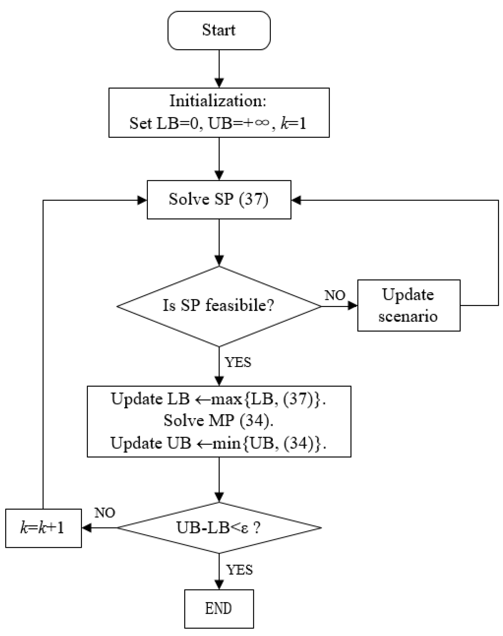
4. Solution Strategy

The basic algorithms and corresponding optimization software for solving MINLP problems are summarized in [41], where it provides ideas for effectively solving different types of MINLP problems. Decomposition method is used to rewrite the RDB-DRER problem (33) as:

$$\begin{array}{l}\min {\mathit{c}}^T\mathit{x}+\mu \\ s.t.\mathit{A}\mathit{x}-\mathit{b}\le 0\\ z_i^g\in \{0,1\}\end{array}$$

(34)

where (34) is called master problem (MP).

$$\begin{array}{l}\mu =\lambda \log {\mathbb{E}}_{P_0}\left[e^{Q\left(\mathit{x},\mathit{\xi }\right)/\lambda }\right]+\lambda \eta \\ s.t.\mathit{T}\mathit{y}+\mathit{W}\mathit{x}\le \mathit{d}-\mathit{R}\mathit{\xi }\\ \mathit{x}\ge 0,\mathit{y}\ge 0\end{array}$$

(35)

where (35) is called subproblem (SP).

In order to emphasis $\left(x,\lambda \right)$ is the joint decision vector, $\mu \left(\mathit{x},\lambda \right)$ is used rather than ${\mu }_x\left(\lambda \right)$ to denote the objective function (35) for brevity:

$$\underset{x\in X,\lambda \ge 0}{\min }\mu \left(\mathit{x},\lambda \right):=\lambda \log {\mathbb{E}}_{P_0}\left[e^{Q\left(\mathit{x},\mathit{\xi }\right)/\lambda }\right]+\lambda \eta .$$

(36)

Suppose $Q\left(\mathit{x},\mathit{\xi }\right)$ is convex in X for every $\mathit{\xi }$. The function $\mu \left(\mathit{x},\lambda \right)$ is a convex function of $\left(\mathit{x},\lambda \right)$. Note that the first term of $\mu \left(\mathit{x},\lambda \right)$ is the logarithmic moment generating function of $Q\left(\mathit{x},\mathit{\xi }\right)$ under the probability measure P₀. In some cases, $Q\left(\mathit{x},\mathit{\xi }\right)$ has a closed-form expression and the problem (36) can be transformed to a deterministic convex optimization problem. But this situation is generally difficult to achieve.

In this paper, assume the closed-form expression of the logarithmic moment generating function is not available, thus (36) is a typical stochastic optimization problem with a fixed probability distribution P₀ [2]. Standard stochastic optimization technique can be used to solve (36) such as the sample average approximation [13] and stochastic approximation. To apply the SAA method, we generate an independent and identical distribution sample from the distribution P₀, and we use the following optimization problem to approximate problem (36), which can be written as the following form:

$$\underset{x\in X,\lambda \ge 0}{\min }{\widehat{\mu }}_K\left(\mathit{x},\lambda \right):=\lambda \log \left(\frac{1}{K}{\displaystyle \sum _{k=1}^K{e}^{Q\left(\mathit{x},{\mathit{\xi }}_k\right)/\lambda }}\right)+\lambda \eta .$$

(37)

Then, the problem (33) can be transformed into (38) as:

$$\begin{array}{l}\underset{\lambda \ge 0,x}{\min }{c}^{T}x+\lambda \log \left(\frac{1}{K}{\displaystyle \sum _{k=1}^K{e}^{Q\left(\mathit{x},{\mathit{\xi }}_k\right)/\lambda }}\right)+\lambda \eta \\ s.t.\mathit{A}\mathit{x}-\mathit{b}\le 0\\ \mathit{T}\mathit{y}+\mathit{W}\mathit{x}\le \mathit{d}-\mathit{R}{\mathit{\xi }}_{\mathcal{S}}\\ \mathit{x}\ge 0,\mathit{y}\ge 0\\ \lambda \ge 0\\ \forall s=1,2,\cdots \mathcal{S}\\ z_i^g\in \{0,1\}\end{array}$$

(38)

Problem (38) can be solved with the existing commercial solver. The procedure to solve the energy and reserve dispatch problem is summarized in Algorithm 1 and the flow chart of the algorithm is described in Figure 1.

Algorithm 1 Energy and Reserve Dispatch.

1: Collect historical data regarding variable uncertainties; 2: Construct the uncertainty set using KL divergence method; 3: Design an empirical distribution using (20) and (21); 4: Reformulate the energy and reserve dispatch problem into (33); 5: Decompose the optimization problem into (34) and (35); 6: Use the SAA method to approximate problem (36); 7: Solve problem (38).

5. Case Study

In this section, all tests are performed on a personal computer (Intel Core i5-8250U 1.8GHz CPU, 8GB RAM). Programs are coded using MATLAB R2016a. The problem is solved by CPLEX 12.5.1 combined with YALMIP. The 6-bus system and IEEE 118-bus system are used to test the method proposed.

5.1. 6-Bus System

Configuration of the 6-bus system is shown in Figure 2. This 6-bus system consists of three thermal units, two renewable energy resources (wind farm), seven transmission lines, and three loads, with detailed data in [32].

We assume that the true distribution of the variable renewable energy power forecast errors obeys a normal distribution, with the mean of 0 and standard deviation of 0.1. We apply the Monte Carlo method to generate 500 scenarios as hypothetical data.

We give the following robust optimization mathematical model and stochastic optimization mathematical model to compare the proposed DRO method.

(1) Robust model:

$$\begin{array}{l}\min {\mathit{c}}^T\mathit{x}+\underset{s\in \{1,2,\cdots ,S\}}{\max }{\mu }_s\\ s.t.\mathit{A}\mathit{x}-\mathit{b}\le 0\\ z_i^g\in \{0,1\}\end{array}$$

(39)

(2) Stochastic model:

$$\begin{array}{l}\min {\mathit{c}}^T\mathit{x}+{\displaystyle \sum _{s=1}^S{\rho }_s{\mu }_s}\\ s.t.\mathit{A}\mathit{x}-\mathit{b}\le 0\\ z_i^g\in \{0,1\}\end{array}$$

(40)

In the following numerical analysis, if there is no special explanation, value of the ambiguity index $\eta$ is set to 0.3 and the confidence level $\alpha$ is 0.95.

The predicted data of renewable energy output are given in Figure 3. The structure of the uncertainty sets in the RO model include interval set, polyhedral set, and ellipsoidal set, etc. In order to simplify the calculation and compare the results obvious, the uncertainty set of RO model is interval uncertainty set as shown in Figure 3.

Table 1. Comparison of the results obtained by three methods.

		RO	SO	DRO
First-stage objective value ($)	Generation cost ($)	5351.53	4927.80	4869.58
	Reserve cost ($)	124.71	140.95	174.39
Second-stage objective value ($)		685.94	412.62	538.75
Total objective value ($)		6162.18	5481.37	5582.72

shows the comparison of the results obtained by three different methods. From the table, we can see the total objective value of RO is the largest. The reason is that RO just considers the worst-case which happened in the second-stage problem, where the value of RO is the largest too. In SO, the expected cost is considered in the second-stage problem, and the objective value is the smallest. As to DRO, its objective value is larger than that of SO and is smaller than that of RO, since the second-stage problem of DRO is a combination of stochastic and robust optimization. The value of reserve cost obtained by DRO is larger than those of RO and SO, while its generation cost is the smallest. DRO combines RO and SO, which makes it less conservative, which is demonstrated by numerical results.

The relationship of objective value and number of scenarios is depicted in Figure 4. With the increase of scenario quantity, the uncertainty sets of robust optimization become larger with larger objective values obtained by RO. Meanwhile, the objective of SO or DRO almost remain the same value under different sample sizes, because the characteristic of RO just considers the worst-case. As the number of scenarios increases, more scenarios are taken into account, making the worst-case scenario change. At the same time, the trend of SO and DRO shows that these two methods make better use of available data. Moreover, for large sample size, the result of DRO is close to that of SO.

Figure 5 depicts that with the increases of the ambiguity index η, the objective value increases. The larger ambiguity index denotes that the more distribution functions of the uncertain variables in the ambiguity set. This trend illustrates that the proposed DRO method can utilize the available historical data. At the same time, it can be seen that the growth trend is more and more smooth. The reason is that the influence of the ambiguity index on the objective value is limited, and the trend is getting smaller and smaller. In addition, the curve in Figure 5 also shows that the scale of the historical data is very critical for this method, the larger the scale is, the more exact the ambiguity set is and the less conservative the result is.

5.2. 118-Bus System

IEEE 118-bus system contains 19 generators, 35 synchronous condensers, 177 lines, 9 transformers, and 91 loads with total load demand 5500 MW. Detail data can be obtained from online at http://labs.ece.uw.edu/pstca/pf118/ieee118psp.txt [38]. The same hypothetical historical data of renewable energy resource generation predicted errors are as in the 6-bus system. And other parameters are also the same as those of the 6-bus system.

The relationship between objective value and confidence level is showed in

Table 2. Objective value of DRO with different confidence level.

Number of Scenarios	Confidence Level	Objective Value ($)
500	0.9	63,497.43
500	0.95	63,510.08
500	0.98	63,531.71

. Under the same number of scenarios but with different confidence level, the total objective value has a little difference. The result demonstrates that the confidence level has little relative with the objective value.

To obtain the results given in

Table 3. Operating costs of energy and reserve dispatch.

	RO	SO	DRO
Generation cost ($)	63,502.81	62,420.51	62,453.61
Reserve cost ($)	525.50	282.21	536.57
Re-dispatch cost ($)	2666.52	579.64	519.90
Total cost ($)	66,694.83	63,282.36	63,510.08

;

Table 4. Reserve capacities obtained by different methods.

	Bus	RO	SO	DRO
Up reserve (MW)	10	0	0	74.29
	65	110.87	80	98.99
	66	80	72.76	80
	69	80.99	60	18.71
Down reserve (MW)	65	168	163.06	168
	66	130.62	0	108.43
	87	12.02	17.51	34.33

, RO, SO and DRO are applied to solve the problem. The results of generation cost obtained by the three methods are similar, while the re-dispatch costs obtained by RO is larger than those of SO and DRO, leading to larger total operating costs. The operating cost obtained by DRO is larger than that of SO, since the worst-case scenario is explicitly considered in DRO. The total reserve capacities obtained by RO and DRO are nearly the same, which are larger than that obtained by SO. Therefore, DRO is verified to strike the balance between the efficiency and the reliability of power system operations.

5.3. Discussion

Compared with RO and SO methods, tests in the 6-bus system show the feasibility of the proposed DRO model and it has less conservative than the pure RO model. Results in the 118-bus system also demonstrate that the method proposed can work well. The objective value obtained by DRO is larger than that of SO and is smaller than that of RO, since the worst-case scenario is explicitly considered in DRO. To our best knowledge, the advantage of the DRO approach lies in its robustness to hedge against distributional ambiguity. If the underlying true distribution is invariant and the number of samples is large enough, the ambiguity of probability distribution for the uncertainty is insignificant. Therefore, the advantage of using ambiguity set is not evident. However, when the number of samples is limited or the probability distribution is time-variant, the ambiguity set is remarkable. In this case, the merit of the DRO approach manifests more.

6. Conclusions and Prospects

In this paper, a two-stage DRO model is proposed to address the energy and reserve dispatch problem with renewable energy generation. Based on the Kullback–Leibler divergence and support set, the ambiguity set is constructed to encompass all candidate distributions of renewable energy generation. This ambiguity set is formulated with a variable confidence level, which is granted more flexibility in adjusting the level of conservatism. Thus, a DB-DRER model, which can fully utilize the known historical data, is proposed. To improve its tractability, we derive an equivalent distributionally robust counterpart for the problem by taking advantage of duality reformulation technique to handle the worst-case expectation. Case study demonstrates that the proposed model can work well in the 6-bus system and IEEE 118-bus system.

This paper mainly studies the economic scheduling problem under the uncertainty of renewable energy output. The Kullback–Leibler divergence method is used to model the uncertain variables. In future work, another kind of method, such as Wasserstein distance, can be applied to solve this problem. In addition, we will further investigate the Kullback–Leibler divergence method of considering to balance risk-averse and benefit problem in power systems.

References

1. Manjure, D.P.; Mishra, Y.; Brahma, S.; Osborn, D.L. Impact of Renewable energy Power Development on Transmission Planning at Midwest ISO. IEEE Trans. Sustain. Energy 2012, 3, 845–852. [Google Scholar] [CrossRef]
2. Yang, X.; Song, Y.; Wang, G.; Wang, W. A Comprehensive Review on the Development of Sustainable Energy Strategy and Implementation in China. IEEE Trans. Sustain. Energy 2010, 1, 57–65. [Google Scholar] [CrossRef]
3. van Ackooij, W.; Finardi, E.C.; Ramalho, G.M. An Exact Solution Method for the Hydrothermal Unit Commitment Under Renewable energy Power Uncertainty with Joint Probability Constraints. IEEE Trans. Power Syst. 2018, 33, 6487–6500. [Google Scholar] [CrossRef]
4. Tang, C.; Xu, J.; Tan, Y.; Sun, Y. Lagrangian Relaxation with Incremental Proximal Method for Economic Dispatch with Large Numbers of Wind Power Scenarios. IEEE Trans. Power Syst. 2019, 34, 2685–2695. [Google Scholar] [CrossRef]
5. Hedayati-Mehdiabadi, M.; Zhang, J.; Hedman, K.W. Wind Power Dispatch Margin for Flexible Energy and Reserve Scheduling With Increased Wind Generation. IEEE Trans. Sustain. Energy 2015, 6, 1543–1552. [Google Scholar] [CrossRef]
6. Lai, T.L. Stochastic Approximation. Ann. Stat. 2003, 31, 391–406. [Google Scholar] [CrossRef]
7. Shapiro, A. Sample Average Approximation. In Advertising Response, Encyclopedia of Operations Reseach; Springer: Berlin/Heidelberg, Germany, 2013. [Google Scholar] [CrossRef]
8. Jiang, R.; Guan, Y. Data-driven chance constrained stochastic program. Math. Program. 2016, 158, 291–327. [Google Scholar] [CrossRef]
9. Lopez, C.J.; Ano, O.; Ojeda Esteybar, D. Stochastic Unit Commitment & Optimal Allocation of Reserves: A Hybrid Decomposition Approach. IEEE Trans. Power Syst. 2018, 33, 5542–5552. [Google Scholar]
10. Mavromatidis, G.; Orehounig, K.; Carmeliet, J. Design of distributed energy systems under uncertainty: A two-stage stochastic programming approach. Appl. Energy 2018, 222, 932–950. [Google Scholar] [CrossRef]
11. Zakariazadeh, A.; Jadid, S.; Siano, P. Smart microgrid energy and reserve scheduling with demand response using stochastic optimization. Int. J. Electr. Power Energy Syst. 2014, 63, 523–533. [Google Scholar] [CrossRef]
12. Li, J.; Wang, S.; Ye, L.; Fang, J. A coordinated dispatch method with pumped-storage and battery-storage for compensating the variation of wind power. Prot. Control. Mod. Power Syst. 2018, 3, 21–34. [Google Scholar] [CrossRef]
13. Lu, R.; Ding, T.; Qin, B.; Ma, J.; Fang, X.; Dong, Z. Multi-Stage Stochastic Programming to Joint Economic Dispatch for Energy and Reserve with Uncertain Renewable Energy. IEEE Trans. Sustain. Energy 2019, 1. [Google Scholar] [CrossRef]
14. Ben-Tal, A.; Ghaoui, L.E.; Nemirovski, A. Robust Optimization; Princeton University Press: Princeton, NJ, USA, 2009. [Google Scholar]
15. Ben-Tal, A.; Den Hertog, D.; De Waegenaere, A.; Melenberg, B.; Rennen, G. Robust Solutions of Optimization Problems Affected by Uncertain Probabilities. Manag. Sci. 2013, 59, 341–357. [Google Scholar] [CrossRef]
16. Noureldeen, O.; Hamdan, I. Design of robust intelligent protection technique for large-scale grid-connected wind farm. Prot. Control Mod. Power Syst. 2018, 3, 169–182. [Google Scholar] [CrossRef]
17. Moreira, A.; Street, A.; Arroyo, J.M. Energy and reserve scheduling under correlated nodal demand uncertainty: An adjustable robust optimization approach. Int. J. Electr. Power Energy Syst. 2015, 72, 91–98. [Google Scholar] [CrossRef]
18. Wiesemann, W.; Kuhn, D.; Sim, M. Distributionally Robust Convex Optimization. Oper. Res. 2014, 62, 1358–1376. [Google Scholar] [CrossRef]
19. Tong, X.; Luo, X.; Yang, H.; Zhang, L. A distributionally robust optimization-based risk-limiting dispatch in power system under moment uncertainty. Int. Trans. Electr. Energy Syst. 2017, 27, e2343. [Google Scholar] [CrossRef]
20. Zare, A.; Chung, C.Y.; Zhan, J.; Faried, S.O. A Distributionally Robust Chance-Constrained MILP Model for Multistage Distribution System Planning with Uncertain Renewables and Loads. IEEE Trans. Power Syst. 2018, 33, 5248–5262. [Google Scholar] [CrossRef]
21. Zhang, Y.; Shen, S.; Erdogan, S.A. Distributionally robust appointment scheduling with moment-based ambiguity set. Oper. Res. Lett. 2017, 45, 139–144. [Google Scholar] [CrossRef]
22. Duan, C.; Lin, J.; Fang, W.; Jiang, L. Data-driven Distributionally Robust Energy-Reserve-Storage Dispatch. IEEE Trans. Ind. Inform. 2017, 14, 2826–2836. [Google Scholar] [CrossRef]
23. Li, B.; Jiang, R.; Mathieu, J.L. Distributionally robust risk-constrained optimal power flow using moment and unimodality information. In Proceedings of the 2016 IEEE 55th Conference on Decision & Control, Las Vegas, NV, USA, 12–14 December 2016. [Google Scholar]
24. Ghahramani, M.; Nazari-Heris, M.; Zare, K.; Mohammadi-Ivatloo, B. Energy and reserve management of a smart distribution system by incorporating responsive-loads/battery/wind turbines considering uncertain parameters. Energy 2019, 183, 205–219. [Google Scholar] [CrossRef]
25. Amari, S.I.; Karakida, R.; Oizumi, M. Information Geometry Connecting Wasserstein Distance and Kullback-Leibler Divergence via the Entropy-Relaxed Transportation Problem. Inf. Geom. 2017, 1, 1–25. [Google Scholar] [CrossRef]
26. Li, Y.; Wang, X.; Chao, D.; Guo, J. Data-driven distributionally robust reserve and energy scheduling over Wasserstein balls. IET Gener. Transm. Distrib. 2018, 12, 178–189. [Google Scholar]
27. Hanasusanto, G.A.; Kuhn, D. Conic Programming Reformulations of Two-Stage Distributionally Robust Linear Programs over Wasserstein Balls. Oper. Res. 2018, 2017, 1698. [Google Scholar] [CrossRef]
28. Hou, W.; Zhu, W.; Wei, H.; Hiep, T. Data-driven affinely adjustable distributionally robust framework for unit commitment based on Wasserstein metric. IET Gener. Transm. Distrib. 2019, 13, 890–895. [Google Scholar] [CrossRef]
29. Ning, C.; You, F. Data-driven Wasserstein distributionally robust optimization for biomass with agricultural waste-to-energy network design under uncertainty. Appl. Energy 2019, 255, 113857. [Google Scholar] [CrossRef]
30. Zhu, R.; Wei, H.; Bai, B. Wasserstein Metric Based Distributionally Robust Approximate Framework for Unit Commitment. IEEE Trans. Power Syst. 2019, 34, 2991–3001. [Google Scholar] [CrossRef]
31. Chen, Y.; Guo, Q.; Sun, H.; Li, Z. A Distributionally Robust Optimization Model for Unit Commitment Based on Kullback-Leibler Divergence. IEEE Trans. Power Syst. 2018, 33, 5147–5160. [Google Scholar] [CrossRef]
32. Li, Z.; Wu, W.; Zhang, B. A Kullback-Leibler Divergence-based Distributionally Robust Optimization Model for Heat Pump Day-ahead Operational Schedule in Distribution Networks. IET Gener. Transm. Distrib. 2017, 12, 3136–3144. [Google Scholar] [CrossRef]
33. Bakdi, A.; Bounoua, W.; Mekhilef, S.; Halab, L.M. Nonparametric Kullback-divergence-PCA for intelligent mismatch detection and power quality monitoring in grid-connected rooftop PV. Energy 2019. [Google Scholar] [CrossRef]
34. Li, Y.; Miao, S.; Zhang, S.; Yin, B.; Wang, J. A reserve capacity model of AA-CAES for power system optimal joint energy and reserve scheduling. Int. J. Electr. Power Energy Syst. 2019, 104, 279–290. [Google Scholar] [CrossRef]
35. Wei, W.; Liu, F.; Mei, S. Distributionally Robust Co-Optimization of Energy and Reserve Dispatch. IEEE Trans. Sustain. Energy 2016, 7, 289–300. [Google Scholar] [CrossRef]
36. Guan, Y.; Wang, J. Uncertainty Sets for Robust Unit Commitment. IEEE Trans. Power Syst. 2014, 29, 1439–1440. [Google Scholar] [CrossRef]
37. Tsybakov, A.B. Introduction to Nonparametric Estimation; Springer: Berlin, Germany, 2009. [Google Scholar]
38. Xu, X.; Yan, Z.; Shahidehpour, M.; Li, Z.; Yang, M.; Kong, X. Data-Driven Risk-Averse Two-Stage Optimal Stochastic Scheduling of Energy and Reserve with Correlated Wind Power. IEEE Trans. Sustain. Energy 2019, 1. [Google Scholar] [CrossRef]
39. Heitsch, H.; Römisch, W. Scenario Reduction Algorithms in Stochastic Programming. Comput. Optim. Appl. 2003, 24, 187–206. [Google Scholar] [CrossRef]
40. Hu, Z.; Hong, J. Kullback-Leibler Divergence Constrained Distributionally Robust Optimization. Available online: http://personal.cb.cityu.edu.hk/jeffhong/Papers/HuHong2013_technicalreport.pdf (accessed on 30 September 2019).
41. Liu, M.; Cui, C.; Tong, X.; Dai, Y. Algorithms, softwares and recent developments of mixed integer nonlinear programming. Sci. Sin. Math. 2016, 46, 1–20. (In Chinese) [Google Scholar] [CrossRef]
Figure 1. Flow chart of the algorithm proposed.
Electronics 08 01454 g001
Figure 2. Configuration of the 6-bus system.
Electronics 08 01454 g002
Figure 3. Interval uncertainty set of RO.
Electronics 08 01454 g003
Figure 4. Relationship between number of scenarios and objective value.
Electronics 08 01454 g004
Figure 5. Relationship between objective value and index of ambiguity.
Electronics 08 01454 g005