MIMO Radar Using a Vector Network Analyzer

Abstract

In this paper, a multiple-input multiple-output (MIMO) radar system was developed using a Keysight’s N5244A 4-port PNA-X network analyzer and Simulink. The system can transmit and receive TDM stepped-frequency continuous wave signals with a total sweep bandwidth of 450 MHz. The system also provides a reliable, self-contained phase-coherent RF front-end across four RF channels, which is a critical requirement for MIMO Radar signal processing algorithms. A Simulink model was built to organize the collected S-parameters into a virtual array and to perform IFFT processing so that range and angle information from targets could be extracted. The experimental results show the ability of the MIMO radar to distinguish between multiple closely spaced targets with a 33 cm range resolution and a 19^o angle resolution.

1. Introduction

The application of multiple-input multiple-output (MIMO) techniques to radar systems has received considerable attention recently [1,2,3,4,5,6,7,8,9,10,11]. Unlike traditional phased-array radars in which a steered beam is used at the transmitter to scan a sector, MIMO radar transmits different waveforms from each omnidirectional antenna element simultaneously, allowing for a sector scan rate that is several times faster than steered beam radars. The waveforms which bear the target information can be extracted by a bank of matched filters at the receiver end. Generally, MIMO radar is implemented through either spatial diversity in antennas or through colocated antennas using orthogonal independently transmitted waveforms [2]. In this paper, only the colocated antenna configuration were examined [7,8,9,10,11]. It has been shown that this kind of radar system has many advantages such as an excellent clutter interference rejection capability [7], improved parameter identifiability [8], and enhanced flexibility for transmitting beampattern design [10,11]. One interesting application of collocated MIMO radars is their use in navy ships to detect multiple surface targets, in both littoral and open ocean, that have small radar-cross sections and become increasingly difficult to detect when there are significant sea clutter environments [12,13,14,15]. With collocated MIMO radar, a ship can detect these targets with an excellent clutter interference rejection capability and maintain its radar picture with a fast refresh rate to provide precious battle space and reaction time to fight.

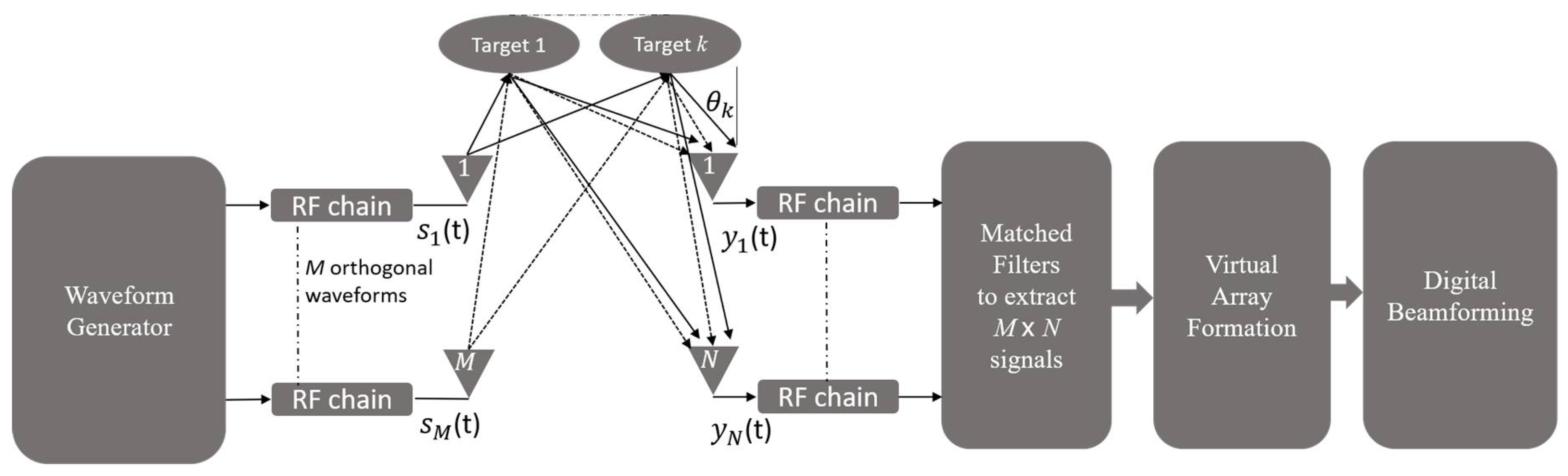
A generic MIMO radar design is illustrated in Figure 1, where there are M independent orthogonal transmitters and N receivers. Each receiver would have M matched filters that correspond to the M distinct transmitted waveforms. Having M independent transmitters and N receivers produces MN paths for the return from the k^th target, which, in turn, creates a virtual array with a larger effective aperture than the physical array. The received signal for the system illustrated in Figure 1 is given by [2,5]

$$y_n\left[n\right]={{\displaystyle \sum }}_{k=1}^K\alpha \left({\theta }_k\right){{\displaystyle \sum }}_{m=1}^M{e}^{-j{\omega }_c{\tau }_{mn}\left({\theta }_k\right)}{s}_m\left[n\right]+w_n\left[n\right],$$

(1)

where α is the complex amplitude of the k^th return signal from a target located at an angle ${\theta }_k$, $s_m$ is the baseband samples of the m^th transmitted signal, ${\tau }_{mn}\left({\theta }_k\right)$ is the total phase delay between the m^th transmitting element, the k^th target, and the n^th receiver, ${\omega }_c$ is the carrier frequency, [n] is the time index, and $w_n$ is an additive white Gaussian noise with zero-mean and a covariance matrix R_w = σ²I_m. It is important to note in (1) that the MIMO radar takes the sum of returns from all targets, whereas a phased array radar will only have a return from its directed beam.

Using orthogonal signals and matched filters, a MIMO radar can distinguish the received paths independently and can achieve a ubiquitous mode where it is able to search an entire area in only a few short pulses instead of having to scan a beam through the same sector. Separating and distinguishing the independent transmit and receive paths is the most critical step in designing a MIMO radar because these signals form the virtual array, which defines the two-way antenna pattern, and which contains the information necessary to conduct beamforming on reception. Time-division multiplexing (TDM) MIMO was selected as the orthogonal waveform to be implemented in this paper for its simplicity to form a virtual array and to reduce the number of matched filters required on reception.

Although theoretical analysis has shown the benefits of the MIMO radar concept, experimental measurements to demonstrate the feasibility and performance of such systems are of great interest. Recent work has validated the concept of MIMO radar using commercially available software-defined radios (SDRs) such as the USRPs [16,17,18,19]. However, most SDRs are not ideal for deploying phase-coherent MIMO systems because it is difficult to align and synchronize the time and phase responses across multiple radios [16,20]. To circumvent this problem, this paper proposes a more convenient experimental MIMO radar testbed based on Keysight’s N5244A 4-port PNA-X network analyzer [21] and Simulink [22] that can provide a secure, reliable self-contained phase-coherent RF front-end across four RF channels, which is a critical requirement for MIMO Radar signal processing algorithms. The MIMO testbed described herein was designed to transmit and receive TDM stepped-frequency continuous wave signals with a total sweep bandwidth of 450 MHz at a center frequency 8.78 GHz that can be used to explore advanced MIMO radar beamforming techniques and verify range and angle resolutions.

2. Experimental Setup and Measurement Techniques

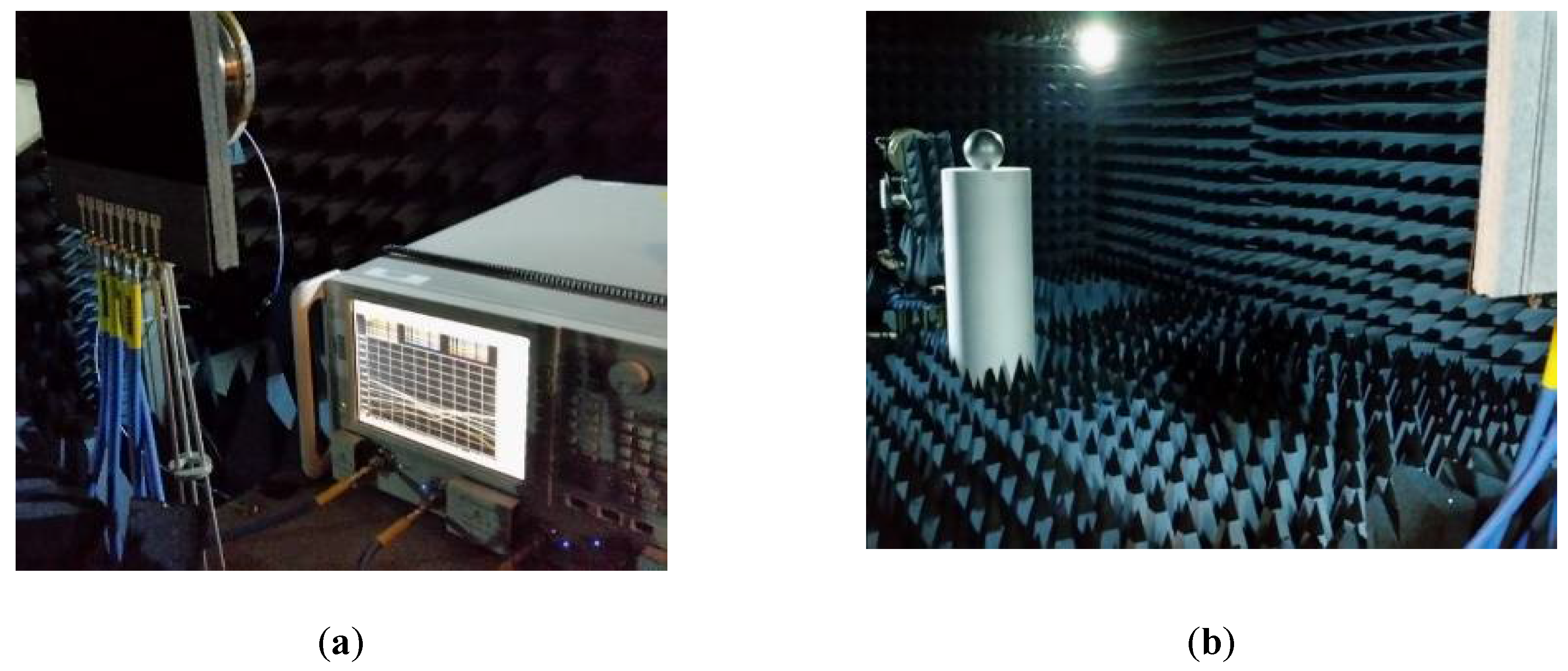
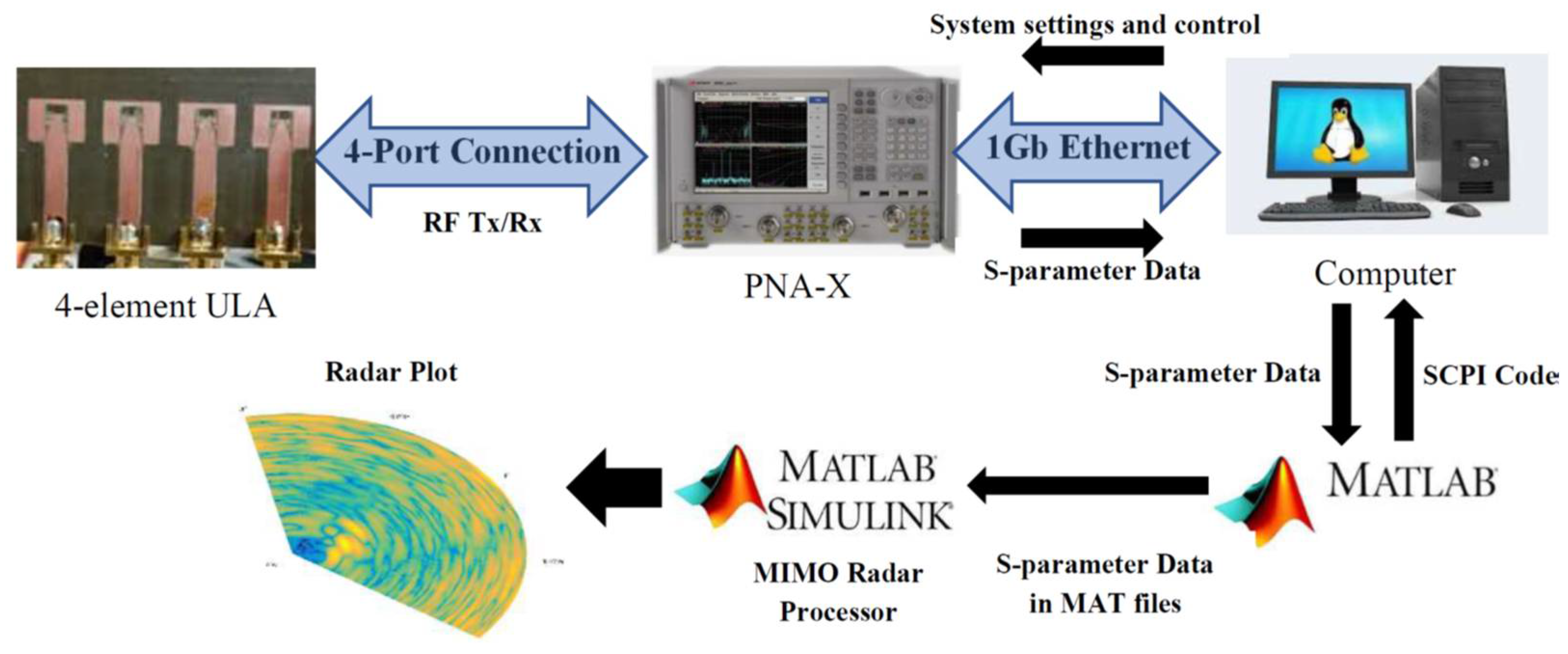
Figure 2 represents a high-level signal flow diagram for the implemented MIMO radar using the Keysight N5244A 4-port PNA-X network analyzer [21]. Given that a network analyzer is specifically built to measure the phase coherent scattering (S) parameters between each of its ports, the instrument is well-suited and convenient to use as the RF front-end for the proposed MIMO system. The N5244A PNA-X is capable of transmitting and receiving stepped-frequency continuous wave signals, in TDM mode, from 10 MHz to 43.5 GHz with a dynamic range of 124 dB and output power of up to13 dBm.

2.1. Antenna Array Design

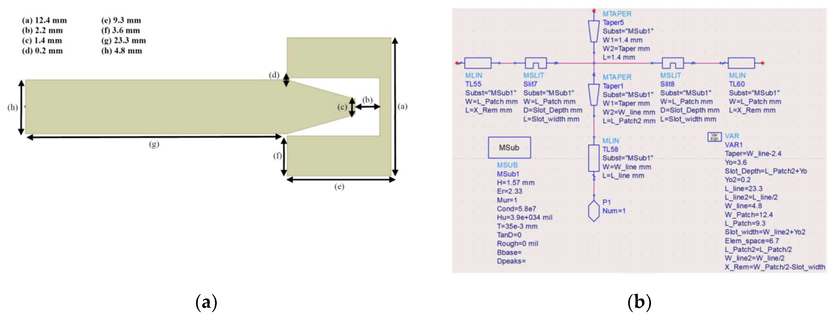
The four test ports of the PNA-X are connected to a four-element microstrip patch antenna array. Microstrip patch antennas were chosen due to their compact size but they are inherently narrowband, which limits the range resolution. Therefore, to extend the bandwidth and improve the range resolution, a U-shaped broadband microstrip patch antenna, [23,24] was designed in Advanced Design System (ADS) [25]. The ADS schematic outlining the dimensions of the antenna is shown in Figure 3. The substrate used to fabricate the antenna is Taconic TLY-3 with a thickness of 1.57 mm and a relative dielectric permittivity, ε_r = 2.33 [26]. The antenna was designed to operate at a center frequency of 8.9 GHz.

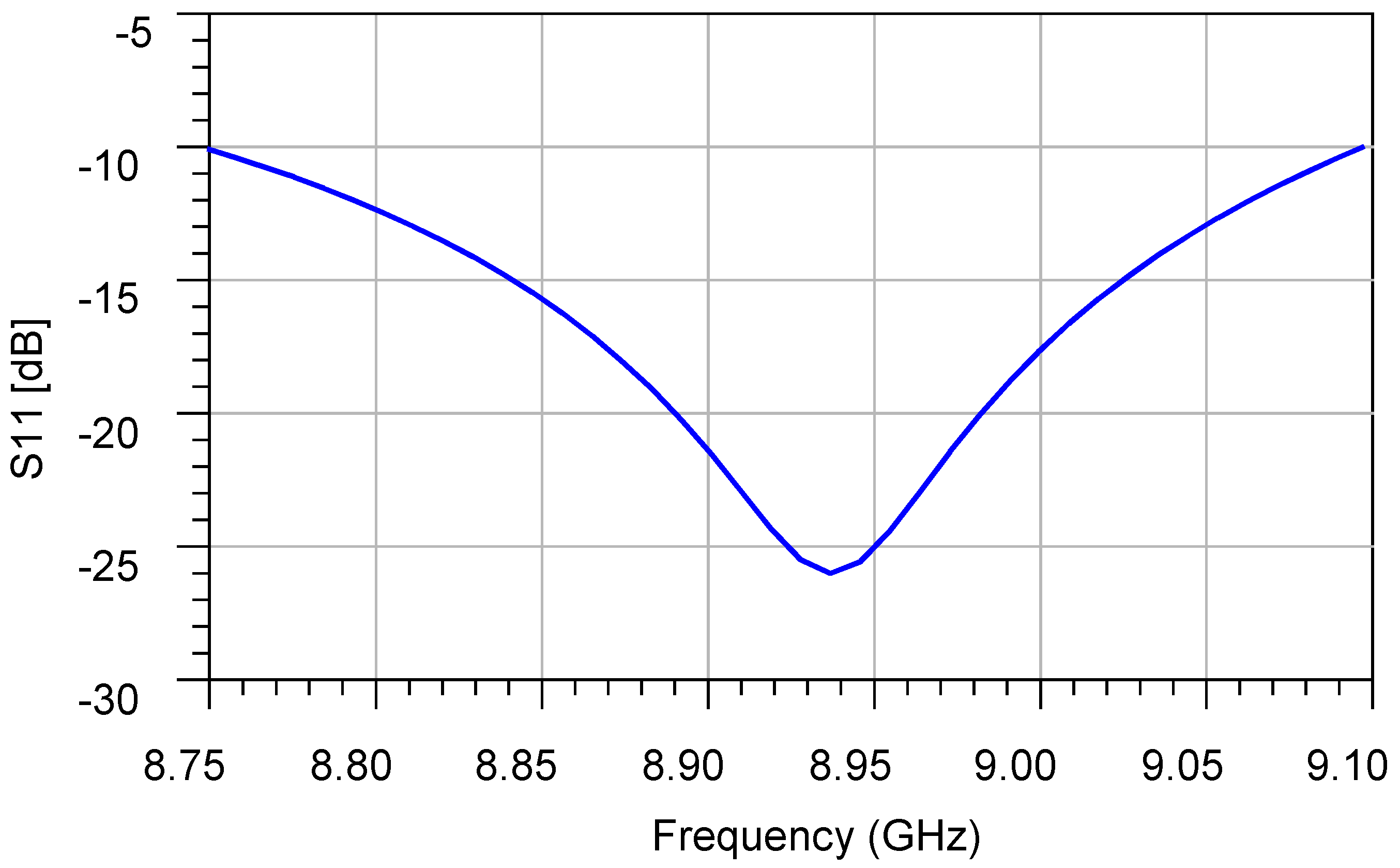
Figure 4 shows the S11 of an isolated single patch with an operational bandwidth of over 350 MHz at –10 dB allowing a range resolution of 43 cm [27]. The U-shaped microstrip patch antenna was designed small enough so that the antenna spacing of the ULA could be set at half wavelength intervals of the center operating frequency.

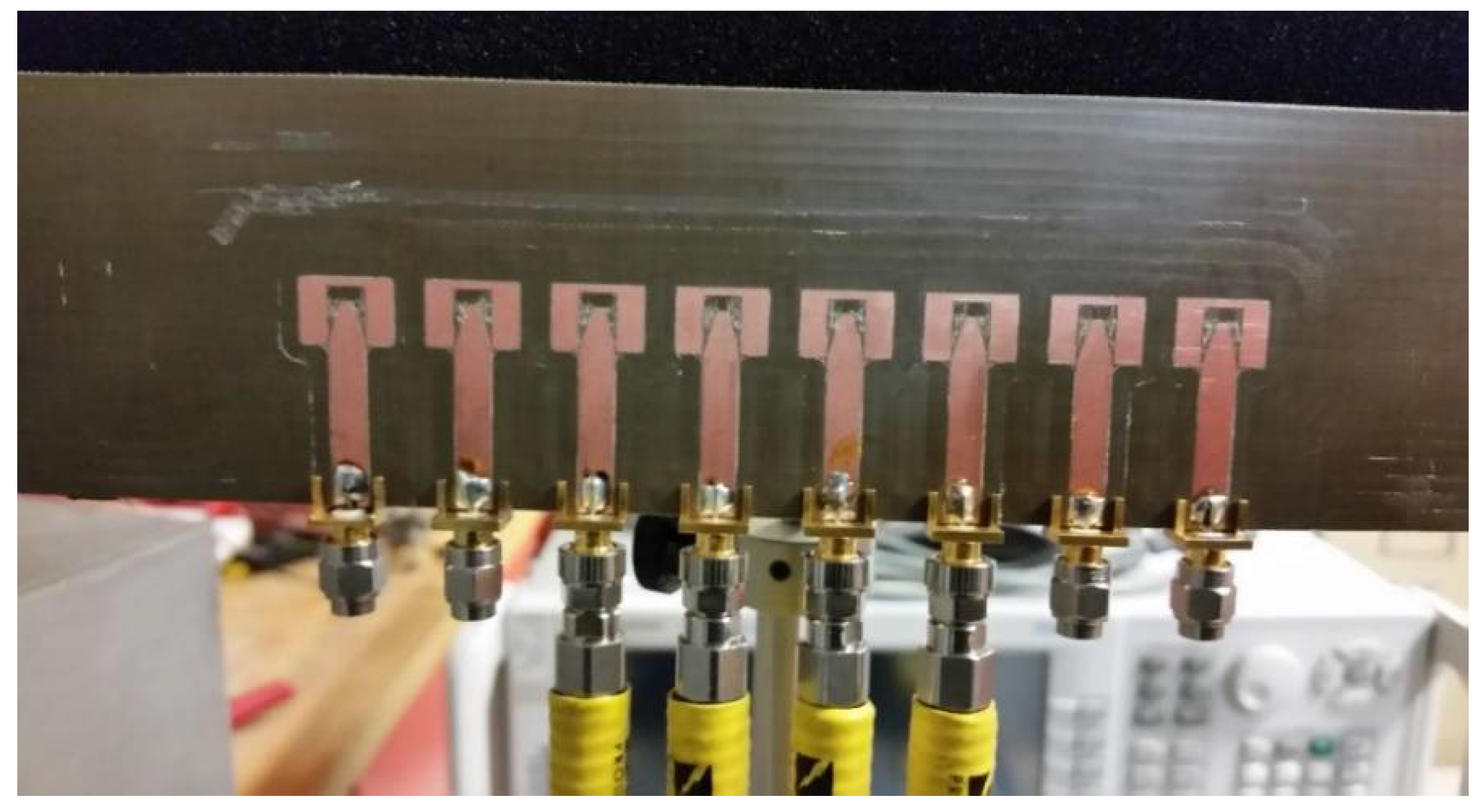
Based on the S11 results of Figure 4, the center operating frequency was set at 8.925 GHz and the antenna spacing was set at 16.8 mm. Although the PNA-X network analyzer only has four ports, an 8-element ULA was fabricated for flexibility and possible future expansion. Figure 5 shows a picture of the fabricated ULA.

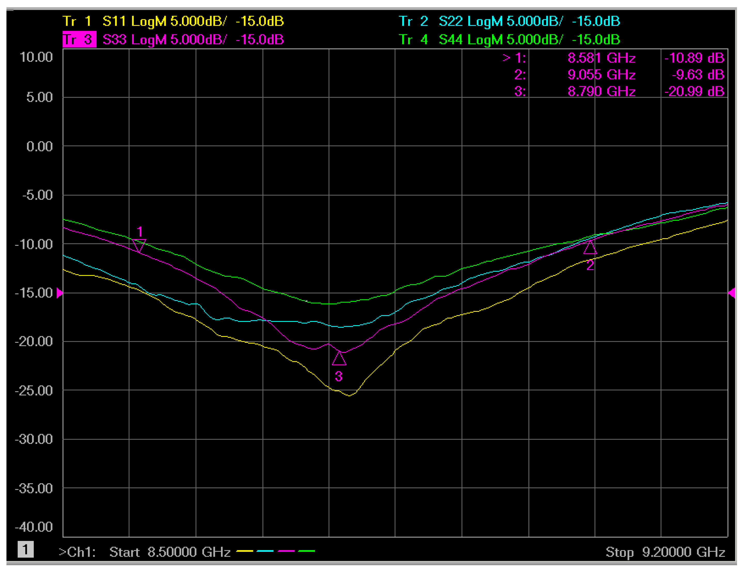
The S-parameters S11, S22, S33, and S44 of four individual elements in the array were measured using the N5244A PNA-X network analyzer. Each element was individually excited, and the rest of the array elements were terminated with 50 Ω matching loads. The results are depicted in Figure 6, where it can be observed that the bandwidth increased for each antenna and that even for the worst measurement, S44, the –10 dB bandwidth increased to approximately 500 MHz compared to 350 MHz of the isolated element. Thus, MC obviously enhances the array bandwidth, which is beneficial for range resolution. It is also noted that the center operating frequency of all elements is approximately the same and shifted around 8.78 GHz compared to 8.925 GHz of the isolated element. The shift in center frequency, increase in bandwidth and differences in S-parameters responses is likely due to the accuracy of the machine that fabricated the ULA and the mutual coupling between antennas that was not accounted for in the isolated element. Therefore, to compensate for the frequency shift, the PNA-X was set to a center operating frequency of 8.78 GHz with a total sweep bandwidth of 450 MHz, providing a 33 cm range resolution. Without frequency compensation, the coupling can cause a target to appear at an angle different than it is in reality and can affect the accuracy of the angular resolution.

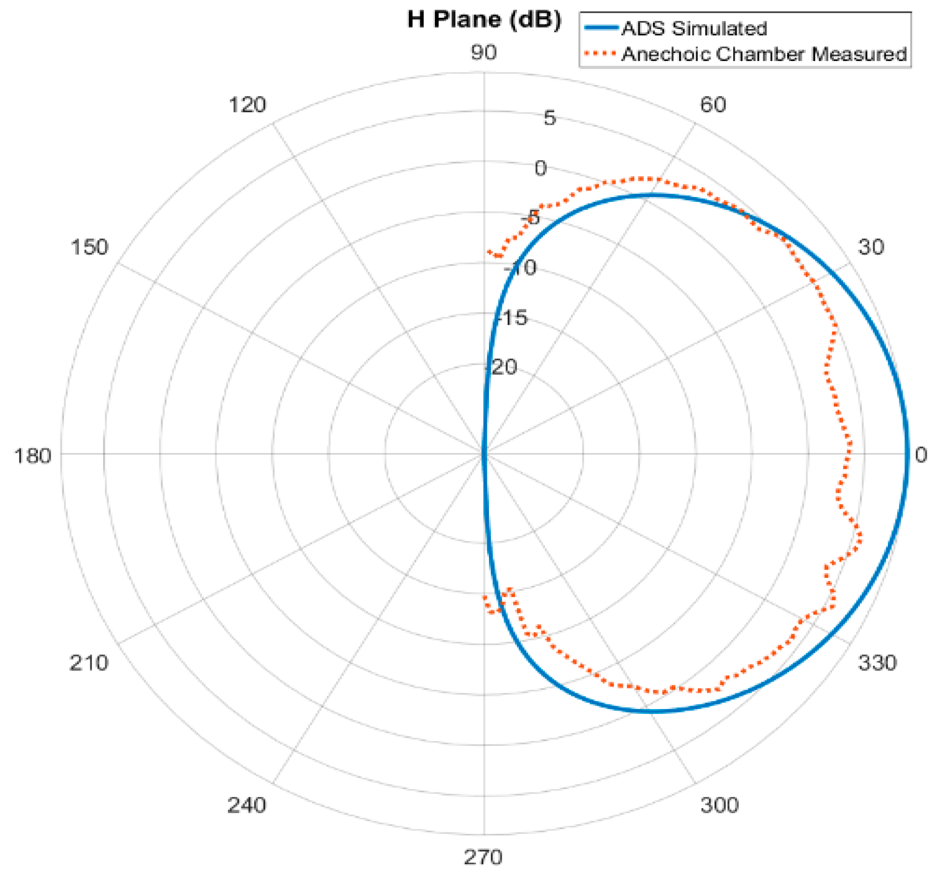
The ULA was mounted on a turret which rotated so that full E and H plane measurements could be taken. Prior to measuring the microstrip patch antenna, a calibration was conducted with a Model 3160 horn antenna at a frequency of 8.8 GHz. Since experimental measurements would primarily be conducted on the H plane using an azimuth radar scan, only H plane measurements are considered. Figure 7 compares the experimental H plane radiation pattern of one element in the array with the isolated element which does not account for the coupling effects. The difference in the antenna pattern and gain could be attributed to the manufacturing accuracy of the machine, the mutual coupling between the closely spaced elements not accounted for in the isolated antenna pattern of the simulation, or from the absorber pad that was placed behind the ULA during measurements. As the main requirement of producing a broadband microstrip patch antenna was met, further antenna testing was not completed as the antenna met the minimum requirements of achieving less than a 1 m range resolution for a stepped-frequency continuous wave waveform MIMO radar.

2.2. System Setting and Control

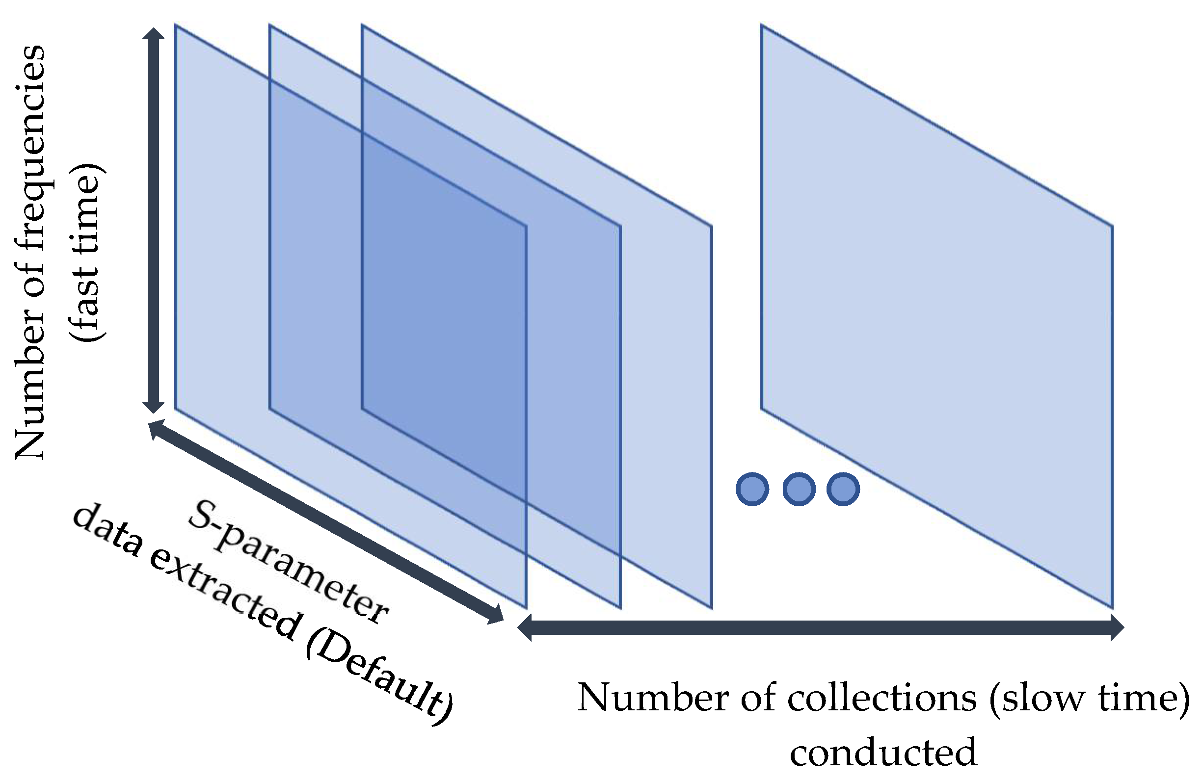
The PNA-X is connected to a Linux computer running MATLAB/SIMULINK [22] through a 1 GB Ethernet cable to form an IP network. The PNA-X is controlled locally from its front panel or remotely from the computer through several MATLAB functions using Standards Commands for Programmable Instruments (SCPI) code [21]. The SCPI MATLAB function adjusts the settings on the PNA-X, such as frequency, IF bandwidth, power settings, number of samples, and the S-parameters to extract. The SCPI MATLAB function will save the S-parameter data in an I and Q format, which can be used as radar returns and can be processed by Simulink. Before running the SCPI MATLAB function, an electronic calibration using the Keysight N4692A ECal module is either performed or recalled from memory to balance the four channels. The S-parameters are organized in a data cube format as shown in Figure 8 and are saved as a MAT file in MATLAB. The first dimension is defined by the number of frequency steps taken over a total specified bandwidth during the frequency sweep (fast time). The total bandwidth will limit the range resolution of the radar and was set to 450 MHz to respect the operational bandwidth of the microstrip uniform linear array (ULA) for all experiments. The second dimension of the matrix is defined by the number of S-parameters that are extracted. If all 16 S-parameters are extracted, which is the default setting, then the length of the second dimension will be 33, which corresponds to the received amplitude and phase for each S-parameter as well as a column for the current operating frequency. Four frequency sweeps are required to measure all 16 S-parameters. The last dimension of the matrix, slow time, is defined as the number of times the PNA-X will collect the specified S-parameters, which may then be used for coherent integration to increase the processing gain.

2.3. MIMO Radar Signal Processing

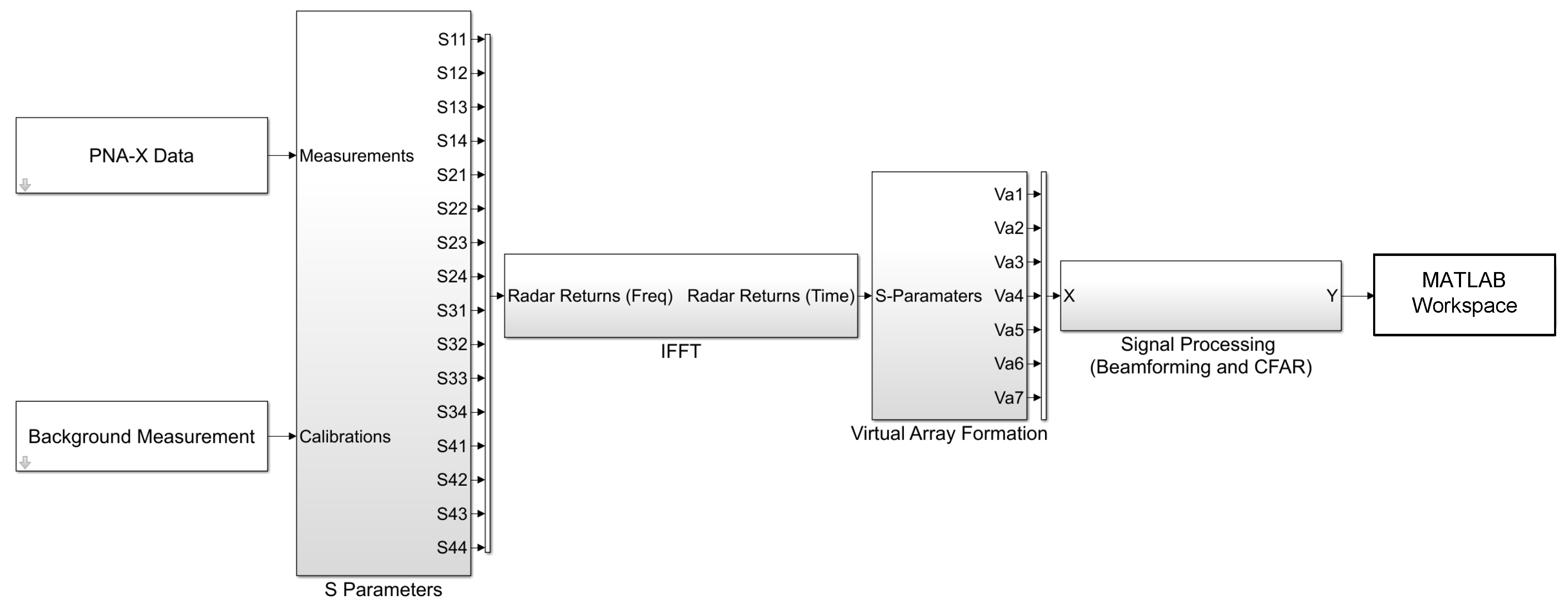
Knowing the format of the received data, a Simulink model was built to organize the S-parameters into a virtual array and to perform IFFT processing and beamforming so that range and angle information from targets could be extracted. The high-level Simulink model used to process the radar returns is shown in Figure 9. In a laboratory setting, clutter may be removed by performing two sets of measurements: one with targets and another one with only the background.

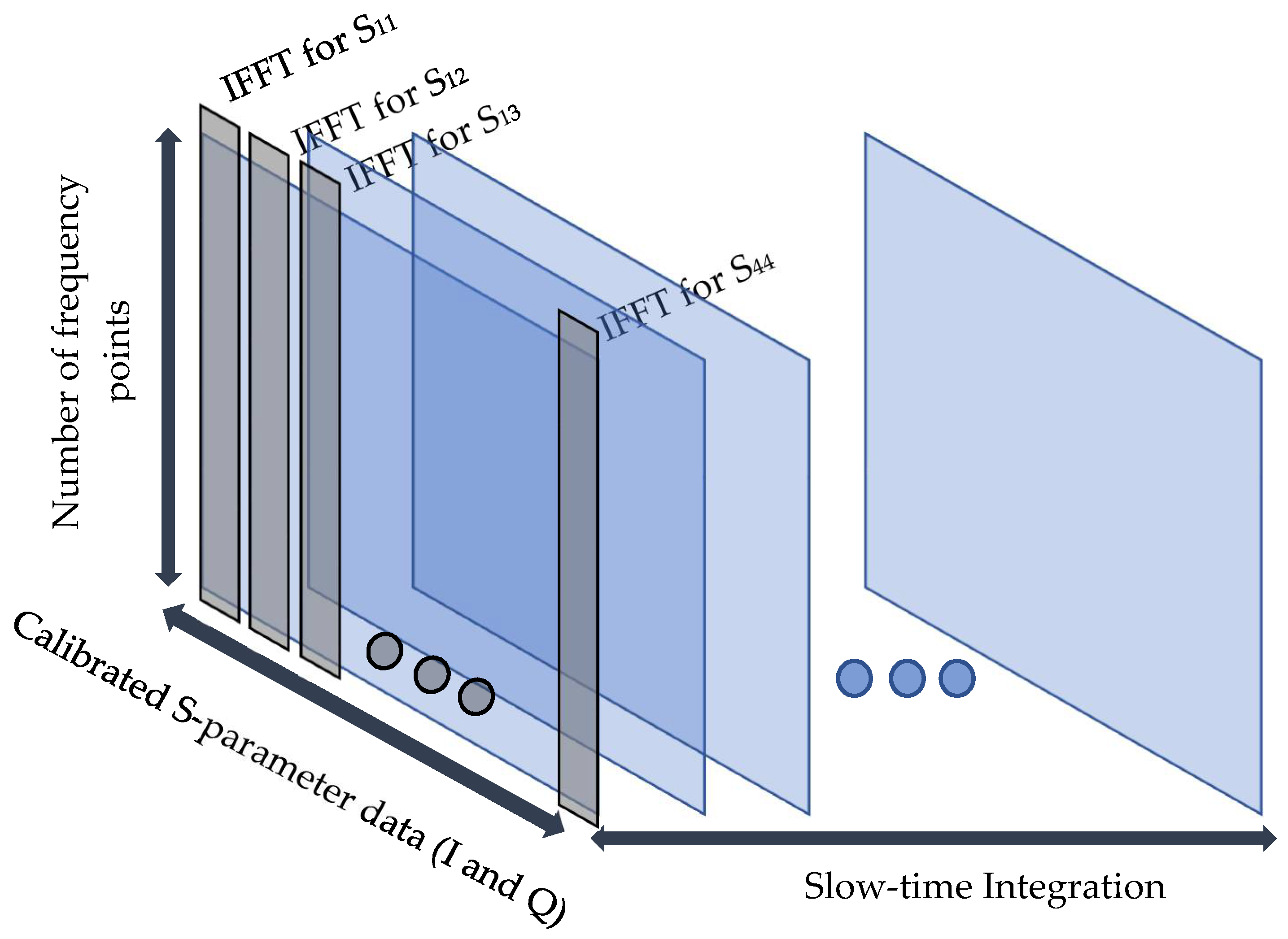
The matrices of the PNA-X Data and Background Measurement from Figure 9 are measured with the same settings to ensure that they have the same matrix dimensions. These two matrices are the input to the Simulink model, which processes the data one sweep at a time. The data from both matrices are sent to the S-parameters block which subtracts the background measurement from the data with targets and converts the received data from amplitude and phase to I/Q data. The I/Q data are then sent to an IFFT block to convert the data from the frequency domain to the time domain. An IFFT is conducted on each S-parameter and then buffered over a specified coherent integration interval. As the data from the PNA-X are stored based on equal steps of frequency, the IFFT input is merely one column of data from the S-parameter matrix. Figure 10 illustrates how the I/Q data are extracted for the IFFT and then integrated. The number of frequency points taken over the sweep bandwidth will define the maximum range of the radar, whereas the number of points taken in the IFFT will define the sample rate of the data in the time domain.

After the S-parameter radar returns are converted to the time domain, they are sent to the virtual array block for coherent integration and to create a virtual array. The virtual array block maps S-parameter data to specific virtual elements using several steps. Firstly, as TDM is being used to create orthogonality between transmitting waveforms, there is no cross-correlation between transmissions and the same waveform is being transmitted across all transmitters at different times. Therefore, only a single matched filter is required for each virtual element for TDM. If simultaneous $M$ transmitted orthogonal waveforms were used, $M$ matched filters would be required. As there is no risk of cross correlation between transmitting waveforms by using TDM, the received signals from individual elements can be mapped directly to a virtual element as follows:

$$Virtual Array\left(x\right)={{\displaystyle \sum }}_{m=0}^{M-1}{{\displaystyle \sum }}_{n=0}^{N-1}\delta \left(x-\left(x_m+x_n\right)\right),$$

(2)

where $M$ and $N$ are the numbers of transmitting and receiving antennas, respectively, $x_m$ and $x_n$ are the physical locations of the m^th transmit element and the n^th receive element.

Since four elements are being used in the MIMO radar system, the minimum coherent processing interval (CPI) to create a virtual array when using TDM is four times the sweep time. Using a 4-element ULA in a monostatic scheme and using the spatial convolution from (2), the received signals will be mapped to virtual elements following the logic rules found in

Table 1. Virtual Array logic for MIMO radar simulation.

Transmitting Element	Receiving Elements
Tx 1	Rx 1	Rx 2	Rx 3	Rx 4
Tx 2		Rx 1	Rx 2	Rx 3	Rx 4
Tx 3			Rx 1	Rx 2	Rx 3	Rx 4
Tx 4				Rx 1	Rx 2	Rx 3	Rx 4
Virtual Array Weights	1	2	3	4	3	2	1

. The result is a 7-element virtual array that will have an identical two-way pattern as the phased array radar’s 4-element array. The virtual array buffers the returns from the four frequency sweeps and then performs a summation of the returns in slow time across each virtual element to form the virtual array.

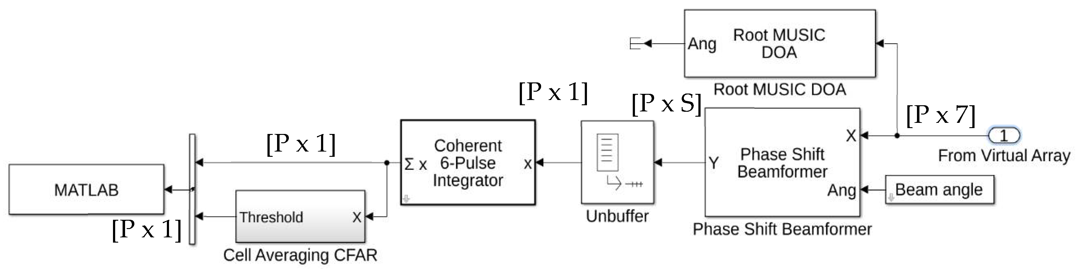
The high-level architecture of the signal processing techniques used in the MIMO radar is depicted in Figure 11. It consists of P range bins and S scan angles using 7-elements virtual array.

Although this paper did not explore high-resolution beamforming techniques such as MUSIC or ESPRIT [27,28,29], a Root MUSIC DOA Simulink block is included in Figure 11 to demonstrate where it could be implemented. The phase shift beamformer block uses the virtual array with appropriate element weights as a reference to perform beamforming. The MIMO radar uses an Unbuffer block to process the radar returns at one scan angle at a time.

2.4. Cell-Averaging CFAR Detector

After coherent integration, the radar returns are sent to a cell-averaging constant false alarm rate (CFAR) detector to determine the presence or the absence of a target. An echo return from a radar will either contain returns from a target plus some interfering noise or just interference such as receiver noise or sea clutter. Interference can cause a radar to miss detecting a real target or can sometimes lead to detecting false targets. The probability of either of these occurring depends on the SNR, which is the ratio of the return signal strength and the variance of the noise level. Therefore, the SNR will define the probability of a target being above a specific threshold, or probability of detection, P_D, as well as the probability of the noise creating a false alarm above that same threshold, P_FA.

Selecting the proper detection threshold is done through random process modeling and statistical analysis where a single target detector must decide between two hypotheses [30]:

$$\begin{array}{l}{H}_0:y=w\\ H_1:y=z+w\end{array}$$

(3)

where H₀ is the null hypothesis representing the background white Gaussian noise $w$, and H₁ is the target return $z$ plus noise. The received radar signals are considered Gaussian random processes; therefore, two probability density functions (PDFs) can be defined as p_y(y|H₀) and p_y(y|H₁). Figure 12 illustrates an example of both PDFs depicting the areas associated with different probabilities [27]. The distance separating the means of the two PDFs is related to the SNR. Increasing the SNR will further separate the two PDFs, lowering the overlap between them, thus increasing P_D and lowering P_FA. Another method to increase the SNR is to lower the variance of the noise as this will also reduce the amount of overlap between the two PDFs. For any radar measurement, y, the generalized likelihood ratio test (GLRT) decision rule can be applied [31]:

$$\frac{p_y(y|H_1)}{p_y(y|H_0)}{\gtrless }_{H_o}^{H_1}{T}_{\mathsf{\Lambda }},$$

(4)

where $T_{\mathsf{\Lambda }}$ is a detection threshold defined for a given P_FA.

It can be shown that (4) can be reduced to form a square law detector [27]:

$${\left|y\right|}^2{\gtrless }_{H_o}^{H_1}T$$

(5)

and that since the magnitude of the noise follows a Rayleigh distribution, the detection threshold, T, must satisfy the following equation:

$$T=-{\sigma }_n^2\ln (P_{FA})$$

(6)

where ${\sigma }_n^2$ is the variance of the noise. Generally, a cell-averaging CFAR detector will use (4) to set the threshold for individual resolution cells of the radar. It will do this by measuring the returns of neighbouring cells to determine ${\sigma }_n^2$ and apply it to (4) with a user-defined P_FA. Guard cells are commonly used around the cell under test so that if a target is present, it does not artificially increase ${\sigma }_n^2$.

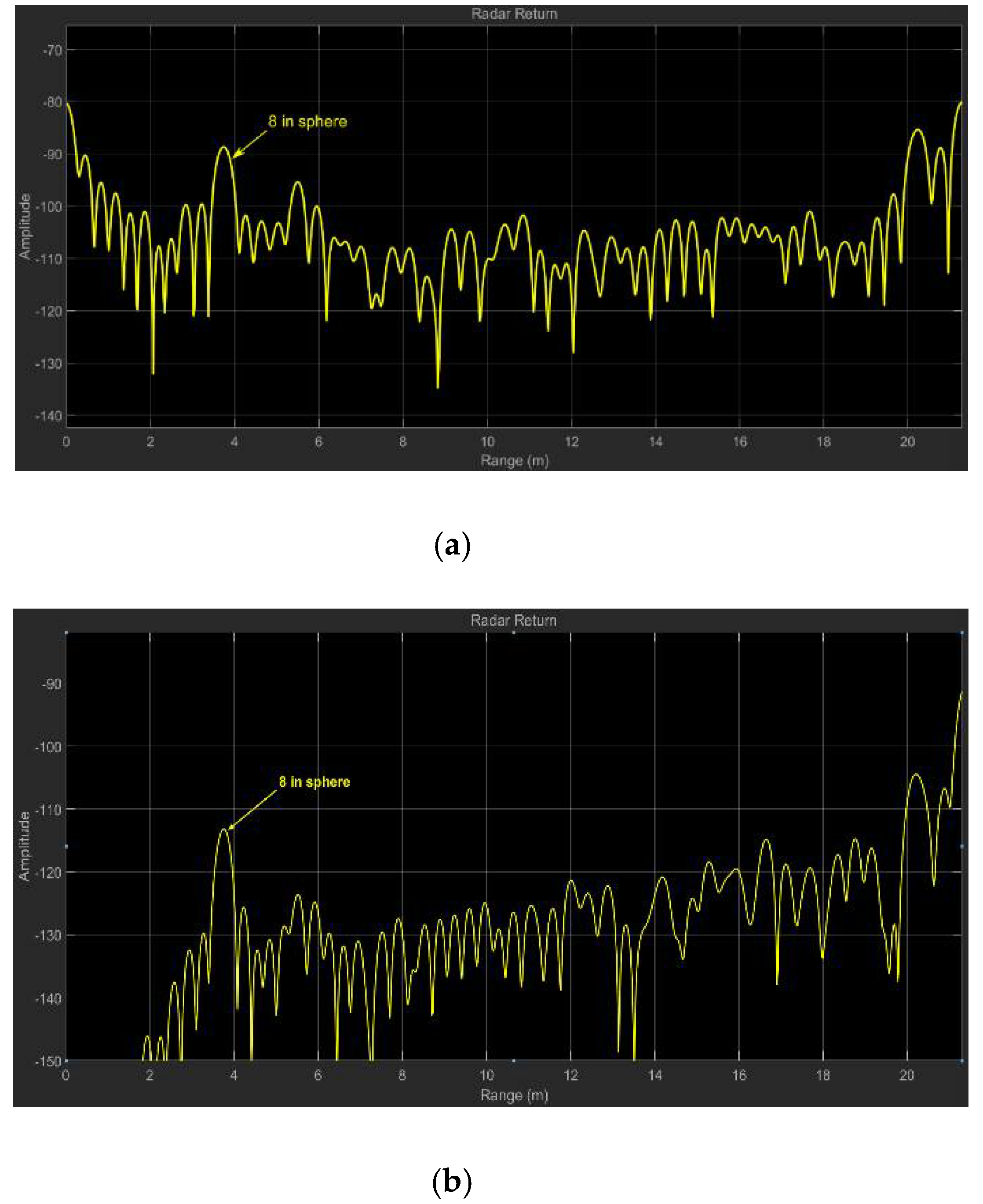
After the coherent integration and CFAR detector, the processed MIMO radar returns are sent to MATLAB’s workspace for plotting and analysis.

3. Experimental Results

The PNA-X was set to a center operating frequency of 8.78 GHz with a total sweep bandwidth of 450 MHz to respect the operational bandwidth of the microstrip ULA for all the experiments. The IF bandwidth of the PNA-X was set at 100 kHz, while a total of 64 frequency samples were taken across the 450 MHz frequency band. The total bandwidth and the number of frequency samples will define the range resolution and unambiguous range of the radar.

3.1. Single target detection

As a first experiment, a single 8-inch diameter aluminum sphere was placed 3.8 m away from the ULA within an anechoic chamber.

The PNA-X and ULA setups in the anechoic chamber are depicted in Figure 13, and the target can be viewed in Figure 14. Figure 14a demonstrates that after 10 coherent integrations, the 8-inch sphere is easily detected over the noise floor. Figure 14b, on the other hand, shows that the nearby returns can be further attenuated using sensitivity time control (STC) [30]. Lastly, Figure 15 depicts the three-dimensional radar return where the 8-inch sphere is detected and exceeds the CFAR threshold.

3.2. Range Resolution

The stepped-frequency waveform achieves a high range resolution by generating synthetic Doppler frequencies by cycling through a band of transmission frequencies [30]. Radar returns are received and initially processed in the frequency domain before an Inverse Fast-Fourier transform (IFFT) is used for range calculations and beamforming.

The Rayleigh range resolution, $\Delta r_{sf}$, for a stepped-frequency waveform is defined as [27]

$$\Delta r_{sf}=\frac{c}{2B_s}$$

(7)

where $B_s=N_s\Delta f_s$ is the total sweep bandwidth of the stepped-frequency waveform, $N_s$ is the number of frequency steps, and $\Delta f_s$ is the step size.

As an IFFT is required to determine range, the maximum range that can be measured before ambiguities exist is N times the range resolution,$\Delta r_{sf}$. Therefore, the unambiguous range,$\Delta r_{unamb}$, of a stepped-frequency waveform is defined as [30]

$$\Delta r_{unamb}= \frac{c}{2\Delta f_s}$$

(8)

According to (7) and (8), a total of 64 frequency samples taken across a sweep bandwidth of 450 MHz corresponds to a range resolution of 33 cm and an unambiguous range of just over 21 m. To confirm the 33 cm range resolution of the radar, two identical targets were used to ensure the same values of radar cross-section (RCS). The targets used were two cylindrical metallic objects with the equivalent dimensions of a standard 355 ml soda can. The cylinders were mounted on two foam mounts at slightly different elevations so that there was a direct line of sight (LOS) path to both targets from the ULA.

The settings for the MIMO radar remained unchanged from the previous experiment, so the theoretical range resolution is 33 cm. Two experiments were conducted with the targets spaced 34 cm and 40 cm apart. The first target was placed at a range $R_1=3.9\mathrm{m}$ from the ULA at −4^o in azimuth and was used as the reference. The second target was placed at the appropriate distance behind the first target and approximately 20 cm higher in elevation. The experimental radar returns were compared to the theoretical values given by [31]

$$Signal\left(n\right)=A_{1n}{e}^{-\frac{i(2\pi \left(2R_1\right)}{{\lambda }_n}}+A_{2n}{e}^{-\frac{i(2\pi \left(2R_2\right)}{{\lambda }_n}},$$

(9)

where Signal(n) is the total theoretical radar return of the two targets for the n^th frequency, n = 1, …, 64. $A_{1n}$ and $A_{2n}$ are the amplitudes of the return signals and they were both set to one for plotting purposes. $R_1$ and $R_2$ are the ranges of the first and the second target, respectively. The ranges are multiplied by two to account for a two-way travel distance. ${\lambda }_{\mathrm{n}}$ is the wavelength for the n^th operating frequency. The 64 returns from Signal(n) undergo an IFFT, which is used as the theoretical reference for comparison with the experimental data.

Figure 16 compares the normalized experimental output of the MIMO radar system with the normalized expected theoretical return for target separation of 40 cm and 34 cm. For a target separation of 40 cm, it can be observed from Figure 16(a) that the experimental data closely align with theoretical values. The higher experimental clutter downrange from the targets is due to other objects and the walls of the anechoic chamber. More specifically, there is a –4 dB null between the two radar targets, meaning that they are distinguishable from one another. One unexpected result was that the target further away had a 2 dB higher return than the closer target. This result is likely due to the second target being at a higher elevation as the E-plane element pattern of the microstrip patch antenna has a larger gain at higher elevations. The comparison between the experimental and theoretical results for target separation of 34 cm is illustrated in Figure 16(b), where, once again, the experimental results align with the expected theory. There is less than a 1 dB null between the returns of the two targets, meaning that a tracking algorithm or a radar operator would likely consider the returns from the two targets as one return instead of two. This experiment shows that a MIMO radar follows theoretical range resolutions and that it is not hindered by its processing to distinguish between two targets.

3.3. Angular Resolution

Whereas the range resolution of the radar is defined by the bandwidth of the waveform used on transmission, angular resolution is defined by the beamwidth of the virtual array of the MIMO radar. The same two cylindrical metallic targets were placed at a range of 4 m then separated in azimuth by 19^o in the first experiment and by 36^o in the second experiment. All settings for the PNA-X remained the same as the range resolution tests. As can be observed from Figure 17, for both scenarios, the results of the experimental received pattern agreed with the theoretical one. It is also noted that the two targets are difficult to distinguish when they are separated by 19^o and distinguishable when they are separated by 36^o.

3.4. Multiple Target Detection

Once again, the radar settings remained unchanged from the previous experiments. Here, three aluminum spheres with 6-inch, 8-inch, and 10-inch diameters were used as the targets and arranged in the anechoic chamber, as illustrated in Figure 18.

Using a slow-time coherent integration factor of ten, the PNA-X MIMO radar surveys the entire 120^o search area and detects the three targets above its cell-averaging CFAR threshold. The resultant three-dimensional radar picture with threshold is shown in Figure 19, accompanied by a top-down perspective of the location of the three targets. It is shown that the experimental MIMO radar system can distinguish multiple targets over a large search area with only a small number of radar returns. Although these targets are static and in the controlled environment of an anechoic chamber, this experiment does show the benefit of a MIMO radar being able to detect multiple targets in an area without electronic scanning. It can survey an area faster, thus decreasing the time it takes to detect a target.

4. Conclusions

Through experimentation, it was shown that a four-port network analyzer and Matlab/Simulink can be used to construct and demonstrate a MIMO radar. Using beamforming on receive, the MIMO radar can scan an entire sector in just a few frequency sweeps. The experimental results validate the MIMO radar’s range and angular resolution. Given that the entire system was composed of pre-existing laboratory equipment, the resulting MIMO radar can be used as a convenient platform upon which to investigate different beamforming techniques and detection methods.

References

1. Li, J.; Stoica, P. MIMO Radar Signal Processing; Wiley-IEEE Press: Hoboken, NJ, USA, 2008. [Google Scholar]
2. Sévigny, P. MIMO Radar: Literature Survey of Papers between 2003 and September 2008; TM 2008-333; DRDC: Ottawa, ON, Canada, March 2009. [Google Scholar]
3. Brookner, E. MIMO radars demystified; and their conventional equivalents. In Proceedings of the 2016 IEEE International Symposium on Phased Array Systems and Technology (PAST), Waltham, MA, USA, 18–21 October 2016; pp. 1–10. [Google Scholar]
4. Moo, P.W.; Ding, Z. Tracking Performance of MIMO Radar for Accelerating Targets. IEEE Trans. Signal Process. 2013, 61, 5205–5216. [Google Scholar] [CrossRef]
5. Bekkerman, I.; Tabrikian, J. Target Detection and Localization Using MIMO Radars and Sonars. IEEE Trans. Signal Process. 2006, 54, 3873–3883. [Google Scholar] [CrossRef]
6. Sun, H.; Brigui, F.; Lesturgie, M. Analysis and comparison of MIMO radar waveforms. In Proceedings of the 2014 International Radar Conference, Lille, France, 13–17 October 2014; pp. 1–6. [Google Scholar]
7. Stoica, P.; Li, J. MIMO radar with colocated antennas. IEEE Signal Process. Mag. 2007, 24, 106–114. [Google Scholar]
8. Li, J.; Stoica, P.; Xu, L.; Roberts, W. On parameter identifiability of MIMO radar. IEEE Signal Process. Lett. 2007, 14, 968–971. [Google Scholar]
9. Stoica, P.; Li, J.; Xie, Y. On probing signal design for MIMO radar. IEEE Trans. Signal Process. 2007, 55, 4151–4161. [Google Scholar] [CrossRef]
10. Aittomaki, T.; Koivunen, V. Signal covariance matrix optimization for transmit beamforming in MIMO radars. In Proceedings of the 2007 Conference Record of the Forty-First Asilomar Conference on Signals, Systems and Computers, Pacific Grove, CA, USA, 4–7 November 2007; pp. 182–186. [Google Scholar]
11. Fuhrmann, D.R.; San Antonio, G. Transmit beamforming for MIMO radar systems using signal cross-correlation. IEEE Trans. Aerosp. Electron. Syst. 2008, 44, 171–186. [Google Scholar] [CrossRef]
12. Spyros, P.; John, J.S. Small-Target Detection in Sea Clutter. IEEE Trans. Geosci. Remote Sens. 2004, 42, 1355–1361. [Google Scholar]
13. Xu, X. Low observable targets detection by joint fractal properties of sea clutter: An experimental study of IPIX OHGR datasets. IEEE Trans. Antennas Propag. 2010, 58, 1425–1429. [Google Scholar]
14. Zhou, W.; Xie, J.; Li, G.; Du, Y. Robust CFAR detector with weighted amplitude iteration in nonhomogeneous sea clutter. IEEE Trans. Aerosp. Electron. Syst. 2017, 53, 1520–1535. [Google Scholar] [CrossRef]
15. Li, Y.; Yang, Y.; Zhu, X. Target detection in sea clutter based on multifractal characteristics after empirical mode decomposition. IEEE Geosci. Remote Sens. Lett. 2017, 14, 1547–1551. [Google Scholar] [CrossRef]
16. Ettus Research-The Leader in Software Defined Radio (SDR). Available online: https://www.ettus.com/ (accessed on 9 October 2019).
17. Aloi, G.; Loscrì, V.; Borgia, A.; Natalizio, E.; Costanzo, S.; Pace, P.; Di Massa, G.; Spadafora, F. Software defined radar: Synchronization issues and practical implementation. In Proceedings of the 4th International Conference on Cognitive Radio and Advanced Spectrum Management, Barcelona, Spain, 26–29 October 2011. [Google Scholar]
18. Braun, M.; Müller, M.; Fuhr, M.; Jondral, F.J. A USRP-Based Testbed for OFDM-Based Radar and Communication Systems. In Proceedings of the 22nd Virginia Tech. Symposium on Wireless Communications, Blacksburg, VA, USA, 30 May–1 June 2012. [Google Scholar]
19. Fernandes, V.N. Implementation of A RADAR System Using MATLAB and the USRP. Ph.D. Thesis, California State University, Northridge, CA, USA, 2012. [Google Scholar]
20. Bathurst, J. Experimental MIMO Radar Design and Results. Chapter 4. Master’s Thesis, Royal Military College of Canada, Kingston, ON, USA, 2017. [Google Scholar]
21. N5244A PNA-X Microwave Network Analyzer, 43.5 GHz|Keysight. Available online: http://www.keysight.com/en/pdx-x201767-pn-N5244A/pna-x-microwave-network-analyzer-435-ghz?cc=CA&lc=eng (accessed on 6 November 2019).
22. Simulink- Simulation and Model-Based Design. Available online: https://www.mathworks.com/products/simulink.html (accessed on 6 November 2019).
23. Chair, R.; Mak, C.L.; Lee, K.-F.; Luk, K.-M.; Kishk, A.A. Miniature Wide-Band Half U-Slot and Half E-Shaped Patch Antennas. IEEE Trans. Antennas Propag. 2005, 53, 2645–2652. [Google Scholar] [CrossRef]
24. Shackelford, A.K.; Lee, K.-F.; Luk, K.M. Design of small-size wide-bandwidth microstrip-patch antennas. IEEE Antennas Propag. Mag. 2003, 45, 75–83. [Google Scholar] [CrossRef]
25. Advanced Design System (ADS) Keysight. Available online: https://www.keysight.com/en/pc-1297113/advanced-design-system-ads?nid=-34346.0&cc=CA&lc=eng (accessed on 6 November 2019).
26. “Taconic: TLY Family of Low Loss Laminates.”. Available online: https://www.4taconic.com/page/tly-87.html (accessed on 6 November 2019).
27. Richards, M.A.; Scheer, J.A.; Holm, W. Principles of Modern Radar: Basic Principles, 1st ed.; SciTech Publishing: Raleigh, NC, USA, 2010. [Google Scholar]
28. Duofang, C.; Baixiao, C.; Guodong, Q. Angle estimation using ESPRIT in MIMO radar. Electron. Lett. 2008, 44, 70–771. [Google Scholar] [CrossRef]
29. Zheng, G.; Chen, B.; Yang, M. Unitary ESPRIT algorithm for bistatic MIMO radar. Electron. Lett. 2012, 48, 179–181. [Google Scholar] [CrossRef]
30. Zhang, X.; Xu, L.; Xu, L.; Xu, D. Direction of departure (DOD) and direction of arrival (DOA) estimation in MIMO radar with reduced-dimension MUSIC. IEEE Commun. Lett. 2010, 14, 1161–1163. [Google Scholar] [CrossRef]
31. Skolnik, M.I. Introduction to Radar Systems, 2nd ed.; McGraw-Hill: New York, USA, 1980. [Google Scholar]
Figure 1. Generic multiple-input multiple-output (MIMO) radar with one target.
Electronics 08 01447 g001
Figure 2. System Overview of PNA-X MIMO radar.
Electronics 08 01447 g002
Figure 3. Broadband U-shaped microstrip patch antenna. (a) Dimensions of U-shaped microstrip patch antenna. (b) Detailed ADS schematic for microstrip patch antenna design.
Electronics 08 01447 g003
Figure 4. Simulated Advanced Design System (ADS) S11 return for a single U-shaped microstrip patch.
Electronics 08 01447 g004
Figure 5. Eight-element ULA built with wideband microstrip patch antennas.
Electronics 08 01447 g005
Figure 6. S-parameter response of 4 microstrip patch antennas.
Electronics 08 01447 g006
Figure 7. H-plane radiation pattern: simulation vs. measurement.
Electronics 08 01447 g007
Figure 8. PNA-X S-parameter MAT file matrix.
Electronics 08 01447 g008
Figure 9. Simulink overview of the PNA-X MIMO radar.
Electronics 08 01447 g009
Figure 10. Manipulation of S-parameters to perform an IFFT and coherent integration.
Electronics 08 01447 g010
Figure 11. MIMO radar signal processing scheme.
Electronics 08 01447 g011
Figure 12. Gaussian probability density functions of noise and a target [27].
Electronics 08 01447 g012
Figure 13. Single target detection: (a) PNA-X and ULA setup in RMC’s anechoic; (b) Metallic 8-inch sphere target located 3.8 m away from the ULA.
Electronics 08 01447 g013
Figure 14. Radar returns from an 8-inch sphere target: (a) Radar return of the first virtual element after 10 coherent integrations; (b) A processed radar return with STC.
Electronics 08 01447 g014
Figure 15. Three-dimensional PNA-X MIMO radar plot with a threshold detector.
Electronics 08 01447 g015
Figure 16. Range resolution verification: (a) target separation 40 cm; (b) target separation 34 cm.
Electronics 08 01447 g016
Figure 17. Experimental and theoretical received patterns of two targets at 4 m: (a) targets separated by 19o; (b) targets separated by 36o.
Electronics 08 01447 g017
Figure 18. Arrangement of three sphere targets in the anechoic chamber.
Electronics 08 01447 g018
Figure 19. PNA-X MIMO radar detection of three targets.
Electronics 08 01447 g019