A Multi-Objective Parallel Iterated Greedy for Solving the p-Center and p-Dispersion Problem

Abstract

This paper generalizes the iterated greedy algorithm to solve a multi-objective facility location problem known as the Bi-objective p-Center and p-Dispersion problem ($BpCD$). The new algorithm is coined as Multi-objective Parallel Iterated Greedy (MoPIG) and optimizes more than one objective at the same time. The $BpCD$ seeks to locate p facilities to service or cover a set of n demand points, and the goal is to minimize the maximum distance between facilities and demand points and, at the same time, maximize the minimum distance between all pairs of selected facilities. Computational results demonstrate the effectiveness of the proposed algorithm over the evolutionary algorithms NSGA-II, MOEA/D, and the Strength Pareto Evolutionary Algorithm 2 (SPEA2), comparing them with the optimal solution found by the $ϵ$-constraint method.

1. Introduction

Facility location is a family of hard optimization problems that have been in the spotlight of the scientific community in the last few years, not only from a theoretical point of view, but also from practitioners in this field [1,2]. Given a set of candidate locations N representing demand points, the goal of this kind of problem is to select a subset of p locations, $P\subset N$, that will host a facility, with the aim of minimizing or maximizing a certain criterion. Demand points (representing customers, patients, students, etc.) will require some kind of services from the facilities (i.e., shopping centers, hospitals, schools, etc.) [3]. Among the most extended criteria are the maximization of dispersion among facilities, which was originally defined in [4], and it has been recently studied in [5], the minimization of the distance between the demand points and their closest facility, defined in [6] and tackled with a totally novel approach in [7], or even the minimization of the distance between the demand points to their closest facility and their second closest facility with the aim of being able to overcome a facility failure. This problem was recently presented and solved with an exact approach [8], but it has also been studied from a heuristic point of view [9].

However, most of these widely accepted criteria do not cover all the real needs since real-world applications usually require considering more than one criterion simultaneously. Nevertheless, in recent years, several works have modeled these real situations as multi-objective problems, being able to tackle more than one objective at the same time. This new approach to deal with the location of facilities is arousing the interest of the scientific community and leading them to model real-world situations accurately. To solve this kind of problem, heuristic or metaheuristic algorithms are recommended since they are a suitable tool to deal with real scenarios in which the quality of the solutions is as important as the speed of finding them.

There are several previous works regarding multi-objective facility location problems. Some of the most interesting papers are briefly described below, where different objectives are considered in each work. For instance, the work in [10] proposed an iterative heuristic for solving a three objective facility location problem. The authors dealt with the p-median problem, the maximum coverage location problem, and the p-center problem simultaneously, by hybridizing exact and heuristic methods. A different work was addressed by [11] to solve the bi-objective obnoxious p-median problem in which the objectives are maximizing the distances between each demand point and their nearest facility and the dispersion among facilities. They presented a multi-objective memetic algorithm and obtained high quality solutions. Another multi-objective location problem was addressed by [12] to solve the p-median p-dispersion problem using a scatter search algorithm. Other approximations are focused on scenarios directly extracted from a real necessity, as [13], where a genetic algorithm was presented for optimizing the location of hospitals in Hong Kong. In [14], a problem with eleven conflicting objectives to locate fire stations in Dubai was presented, considering goal programming to solve it. The locations of hospitals were again considered in [15], where a tabu search metaheuristic was presented for selecting a set of hospitals inside a healthcare network. Finally, the work in [16] modeled the problem of locating casualty collection points by a multi-objective problem with five conflicting objectives. Although all the aforementioned studies dealt with facility location problems, they were specific for the problems described in the corresponding work. However, in the context of heuristic algorithms, the use of specific information about the problem under consideration usually leads to better results [17,18], and therefore, it is interesting to design a new metaheuristic algorithm for dealing with the problem under consideration in this work.

This paper deals with two conflicting objective functions: the minimization of the maximum distance between facilities and demand points (the p-center problem) and the maximization of the minimum distance between all pairs of facilities (p-dispersion problem). The problem is known as the Bi-criteria p-Center and p-Dispersion problem ($BpCD$). The p-center problem and the p-dispersion problem have been widely addressed as single-objective optimization problems by many researches. Specifically, the p-center problem was originally proposed by [19], and it has been the focus of interest of several works. Metaheuristics have been successfully designed to address the p-center problem. For instance, a tabu search and variable neighborhood search algorithm was proposed in [20], while in [21], the problem was tackled by an artificial bee colony optimization algorithm. On the other hand, the p-dispersion problem was defined in [4], and it has been mainly tackled from an exact point of view. In [22], an integer formulation was presented for solving the p-dispersion problem, while in [5], a more efficient and compact formulation for the problem was proposed. Nevertheless, to the best of our knowledge, there are no specific algorithms for solving the multi-objective approach. The current solution consists of adapting some of the most used genetic algorithms for multi-objective optimization (i.e., MOEA/D, NSGA-II, etc.) to solve $BpCD$. However, this adaptation lacks the inclusion of specific knowledge about the problem, resulting in solutions that can be considerably improved, as will be shown in Section 4. Then, it is interesting to design a specific algorithm for obtaining high quality solutions for $BpCD$ in short computing times.

Focusing on $BpCD$, the best and most recent approach for dealing with both objectives at the same time was introduced in [23]. In that work, the authors presented an integer formulation for each considered problem and then an $ϵ$-constraint algorithm for solving the bi-objective problem. Although they were able to provide high quality solutions for $BpCD$, the exact nature of the proposal made the development of new metaheuristics necessary, which were able to reach not only high quality solutions, but also in shorter computing times.

In this paper, we propose the adaptation of the iterated greedy methodology to deal with multi-objective optimization problems. In order to succeed in this goal, we adapted the typical construction/destruction strategies to the multi-objective context. We finally considered that an improvement was found if and only if a point was included in the approximate set of efficient points. The rest of this paper is organized as follows. We first introduce the formal definition of the $BpCD$ problem in Section 2. Then, we describe in Section 3 the algorithm implemented to solve the problem under consideration. Section 4 presents the computational results obtained to test the quality of the proposal and performs a comparison against the NSGA-II algorithm and the $ϵ$-constraint method. Finally, Section 5 summarizes the paper and discusses future work.

2. Problem Definition

Given a set of locations N, with $\left|N\right|=n$, the p-center problem tries to select a subset of $P\subset N$ facilities, with $\left|P\right|=p$, close to the demand points (i.e., those points in the set $N\backslash P$), with the aim of minimizing the distance between each demand point and its closest facility. Given a solution P, the p-center is evaluated as:

$$f_{pC}\left(P\right)\leftarrow \underset{v\in N\backslash P}{max}\underset{u\in P}{min}d(v,u)$$

where $d(v,u)$ is the distance between locations $v\in N\backslash P$ and $u\in P$. Then, the objective of the p-center problem is to find a solution $P_{pC}^{★}$ with the minimum $f_{pC}$ value. More formally,

$$P_{pC}^{★}\leftarrow \underset{P\in \mathbb{P}}{\text{arg min}}{f}_{pC}\left(P\right)$$

$\mathbb{P}$ being the set of all possible combinations of facilities that can be conformed selecting p elements from the set of available locations N.

The p-dispersion problem, on the contrary, is focused on maximizing the distance between the selected facilities, with the aim of distributing the selected facilities over all the available space and avoiding placing facilities close to each other. Given a solution P, the p-dispersion problem is evaluated as:

$$f_{pD}\left(P\right)\leftarrow \underset{u,v\in P,u\ne v}{min}d(v,u)$$

The p-dispersion problem then consists of finding a solution $P_{pD}^{★}$ with the maximum $f_{pD}$ value. Specifically,

$$P_{pD}^{★}\leftarrow \underset{P\in \mathbb{P}}{\text{arg max}}{f}_{pD}\left(P\right)$$

The bi-objective p-center p-dispersion problem, known as $BpCD$, consists of optimizing both objectives simultaneously. It is worth mentioning that these objectives are in conflict, i.e., improving one of them usually results in deteriorating the other one and vice versa. Let us illustrate this fact with an example. Figure 1 and Figure 2 represent the optimal location for the p-center problem and the p-dispersion problem, respectively. This example considers five points, and the aim is to place three facilities. For the sake of clarity, we represent facilities and demand points with squares and circles, respectively. Considering the Euclidean distance, the optimal solution value for the p-center problem is 1.44 units, and the facilities must be located at points $(1,1)$, $(1,4)$, and $(3,2)$. On the contrary, the value for the objective function of the p-dispersion problem is 2.24 units, when considering the same facilities. Analogously, the optimal solution value for the p-dispersion problem is 3.00 units, and the facilities should be placed at points $(1,1)$, $(1,4)$, and $(4,1)$, while the evaluation of the objective function for the p-center problem yields 2.00 units.

As stated in [23] and as we have shown in the example, both objectives are in conflict. Therefore, it is not possible to find a single solution with the optimum value for $f_{pC}$ and $f_{pD}$. For that reason, the output of any algorithm for $BpCD$ is not a single solution, but a set of non-dominated or efficient solutions, also known as the Pareto front. Solutions in the Pareto front are those that cannot be improved in one objective without deteriorating the other one. Formally, a solution $P_1$ dominates another solution $P_2$ if $f_{pC}\left(P_1\right)\le f_{pC}\left(P_2\right)$ and $f_{pD}\left(P_1\right)\ge f_{pD}\left(P_2\right)$ and either $f_{pC}\left(P_1\right)<f_{pC}\left(P_2\right)$ or $f_{pD}\left(P_1\right)>f_{pD}\left(P_2\right)$. The goal in this paper is to find the set of efficient solutions that best approximates the Pareto front, proposing an adaptation of the iterated greedy algorithm to $BpCD$. The main benefit of this adaptation is to provide high quality solutions for $BpCD$ in reasonably short computing times, allowing the algorithm to be considered for real scenarios.

3. Algorithmic Proposal

The methodology used to solve $BpCD$ is based on the iterated greedy metaheuristic proposed in [24]. This metaheuristic has been successfully applied in several optimization problems [25,26,27]. It relies on the repeated execution of two phases: the partial destruction of a solution and its subsequent reconstruction. In the destruction phase, the objective is to explore different regions of the solution space to increase diversification. To this end, some of the elements already included in the solution are removed, even reaching infeasible solutions on some occasions. The final effect is then to move the search procedure to a different region in the space, thus being capable of eventually obtaining better solutions than the previous local optimum. In the reconstruction phase, the destroyed solution is repaired in order to attain a new feasible solution and, probably, a new local optimum with a better value of the objective function. Notice that the solution obtained after the reconstruction phase is not necessarily a local optimum with respect to the considered neighborhood, and therefore, it is recommended to apply a local search procedure to reach a local optimum, bringing to the algorithm a dash of intensification in the generated solutions.

The iterated greedy framework has been traditionally applied to single objective problems, and as far as we know, the generalization of this algorithm to the multi-objective perspective is not widely extended. For instance, the work in [28,29] adapted this methodology to solve different variants of the flow shop scheduling problem. Nevertheless, the iterated greedy algorithm has not been considered in the context of multi-objective location problems. Therefore, it is interesting to redesign the algorithm to make it suitable for dealing with location problems in which more than one objective function must be simultaneously optimized. Our proposal is based on the ideas presented in [30], who proposed an adaptation of the variable neighborhood search methodology for dealing with multi-objective optimization problems. The main contribution of these authors relies on considering the whole approximation front as the incumbent solution of the algorithm. Our adaptation of the iterated greedy methodology to the multi-objective framework is based on the same idea: a solution for $BpCD$ is the complete approximation front, and an improvement is found if and only if the approximation front is modified by inserting new non-dominated solutions. Algorithm 1 shows the pseudocode for the considered Multi-objective Iterated Greedy (MoIG) algorithm.

Algorithm 1$\mathit{MoIG}(N,\widehat{E},\delta ,\mathit{maxNonImprove})$.

1: $\mathit{nonImprove}\leftarrow 0$   2: while$\mathit{nonImprove}\le \mathit{maxNonImprove}$do   3:     ${\widehat{E}}^{\prime }\leftarrow \widehat{E}$   4:     for $P\in {\widehat{E}}^{\prime }$ do   5:         $P^{\prime }\leftarrow \mathit{Destruct}(P,\delta )$   6:         $P^{″}\leftarrow \mathit{Reconstruct}\left(P^{\prime }\right)$   7:         $P^{★}\leftarrow \mathit{LocalSearch}\left(P^{″}\right)$   8:         $\mathit{UpdateFront}({\widehat{E}}^{\prime },P^{★})$   9:     end for 10:     if $\widehat{E}\ne {\widehat{E}}^{\prime }$ then 11:         $\widehat{E}\leftarrow {\widehat{E}}^{\prime }$                ▹ Improvement in the approximation front 12:         $\mathit{nonImprove}=0$ 13:     else 14:         $\mathit{nonImprove}=\mathit{nonImprove}+1$ 15:     end if 16: end while

The algorithm requires four inputs: N, the set of available points to be selected; $\widehat{E}$, the initial set of efficient solutions (see Section 3.1); $\delta$, the proportion of the solution to be destroyed; and $\mathit{maxNonImprove}$, the maximum number of iterations without improvement.

MoIG iterates while not reaching the stopping criterion (Steps 2–16). In each iteration, the algorithm traverses the complete approximation front, alternating the destruction and reconstruction of its solutions (Steps 4–9). In particular, each solution P within $\widehat{E}$ is destructed with the method described in Section 3.2 (Step 5) and then reconstructed following the procedure presented in Section 3.3 (Step 6). The local search that will be described in Section 3.4 is applied to each reconstructed solution (Step 7) in order to improve the solutions. Each improved solution is a candidate for entering in the approximation front under evaluation, ${\widehat{E}}^{\prime }$. If the solution $P^{★}$ is not dominated by any of ${\widehat{E}}^{\prime }$, then it is inserted, removing all those solutions already in ${\widehat{E}}^{\prime }$ that are dominated by the new one $P^{★}$ (Step 8).

Once the main loop of MoIG is finished, ${\widehat{E}}^{\prime }$ contains the remaining non-dominated solutions of the original front, as well as the new non-dominated solutions generated during this iteration. Then, an improvement is found if and only if $\widehat{E}$ and ${\widehat{E}}^{\prime }$ are different (i.e., at least one solution has been included in the approximation front). In that case, the number of iterations without improvement is set to zero, restarting the search. Otherwise, the number of iterations is incremented, continuing until reaching the maximum number of iterations without improvement allowed, used as a stopping criterion (Steps 10–15).

In order to clarify the algorithm proposed for $BpCD$ resolution, we will break down the different phases that make up the algorithm, from the creation of the initial set of solutions used by the iterated greedy metaheuristic to the improvement of these solutions through the application of different local search algorithms.

3.1. Initial Set of Efficient Solutions

The initial set of efficient solutions for the iterated greedy can be generated either at random or using a more intelligent constructive procedure. Although the metaheuristic converges considering random solutions, better results are usually obtained when using a constructive method [31,32].

With the aim of providing the iterated greedy metaheuristic with an initial set of solutions on which to operate, we will leverage the balance between diversification and intensification offered by the Greedy Randomized Adaptive Search Procedure (GRASP) [33]. This methodology consists of two phases that are iteratively repeated: the construction phase to generate a feasible solution and the local search phase to improve that solution. Note that in the context of this problem, two objectives are considered and thus bring us to apply the local search isolatedly with respect to every objective function. Algorithm 2 depicts the pseudocode of GRASP.

Algorithm 2 Construct(N, $\alpha$).

1: $P\leftarrow \varnothing$   2: $\left\{v\right\}\leftarrow \mathit{Random}\left(N\right)$   3: $P\leftarrow P\cup \left\{v\right\}$   4: $\mathit{CL}\leftarrow N\backslash \left\{v\right\}$   5: while$\left|P\right|\ne p$do   6:     $g_{\mathit{min}}=\underset{v\in \mathit{CL}}{\mathit{min}}g(P,v)$   7:     $g_{\mathit{max}}=\underset{v\in \mathit{CL}}{\mathit{max}}g(P,v)$   8:     $\mu \leftarrow g_{\mathit{min}}+\alpha (g_{\mathit{max}}-g_{\mathit{min}})$   9:     $\mathit{RCL}\leftarrow \{v\in \mathit{CL}:g(v)\le \mu \}$ 10:     $u\leftarrow \mathit{Random}\left(RCL\right)$ 11:     $P\leftarrow P\cup \left\{u\right\}$ 12:     $\mathit{CL}\leftarrow \mathit{CL}\backslash \left\{u\right\}$ 13: end while 14: returnP

Traditionally, GRASP selects the first facility at random from the set of available ones, N (Step 2), and this one is included as the initial facility of the solution under construction (Step 3). Then, until selecting p facilities, the algorithm evaluates all the candidates facilities $v\in CL$ with a greedy function $g\left(v\right)$, storing the minimum (Step 6) and maximum (Step 7) values. As we are dealing with a problem where more than one objective must be optimized, the proposed greedy function considers both: $f_{pC}$ and $f_{pD}$. Specifically, we introduce an aggregated greedy function that linearly combines both objectives as follows:

$$g\left(P\right)=\beta ·f_{pC}\left(P\right)-(1-\beta )·f_{pD}\left(P\right)$$

where P consists of the facilities included in the partial solution so far. The parameter $\beta$ controls the weight given to each objective function. On the one hand, values close to zero result in optimizing the p-dispersion problem. On the other hand, values close to one optimize the p-center value. The $\beta$ values considered in this construction are: 0.00, to optimize $f_{pD}$; 0.25, to focus on $f_{pD}$, but slightly taking into account $f_{pC}$; 0.50, to balance $f_{pD}$ and $f_{pC}$; 0.75, to focus on $f_{pC}$, but slightly taking into account $f_{pD}$; and 1.00, to optimize $f_{pC}$. The constructions are applied in this way with the aim of covering the full spectrum of $\beta$ values and get a diverse initial approximation front.

The $\mu$ value (Step 8) is a threshold that any promising candidate must satisfy in order to be included in the restricted candidate list (Step 9). This threshold is computed by considering an $\alpha$ parameter, with $\alpha \in [0,1]$, which controls the greediness/randomness of the search. Specifically, if $\alpha =0$, $\mu$ takes the value $g_{min}$, becoming a totally greedy algorithm. On the contrary, when $\alpha =1$, $\mu =g_{max}$, resulting in a totally random algorithm. Then, this parameter must be carefully selected to reach a balance between greediness and randomness in the construction phase (see Section 4 for a detailed discussion of the parameter value).

The Restricted Candidate List (RCL) is then constructed with those candidates whose greedy function value is smaller than or equal to $\mu$ (Step 9). Once the RCL is generated, any of the candidates is considered as a promising one to become a facility, so the next facility is selected at random (Step 10) from it, updating the candidate list (Step 12). The algorithm ends when p facilities have been selected, returning the constructed solution.

The second phase of GRASP consists of locally improving the generated solution with a local search procedure. In order to define a local search, we first need to define the movement considered in the procedure. For $BpCD$, a swap move is presented, which interchanges a selected facility with a non-selected one. More formally,

$$\mathit{Swap}(P,v,u)\leftarrow (P\backslash \{v\left\}\right)\cup \left\{u\right\}$$

Two local search methods for $BpCD$ are proposed, which basically differ in the optimization criterion. The first one, $L{S}_{pC}$, is focused on optimizing the first objective function, p-center, while the second one, $L{S}_{pD}$, is centered on finding high quality solutions for the second objective function, p-dispersion. Both local search procedures explore the neighborhood defined by those solutions that can be reached by performing a single swap move. In mathematical terms,

$$N_{\mathit{Swap}}\left(P\right)\leftarrow \{P^{\prime }\leftarrow \mathit{Swap}(P,v,u)\forall v\in P\wedge \forall u\in N\backslash P\}$$

In order to avoid biasing the search by performing the swap moves lexicographically, the local search method randomly traverses the neighborhood, performing the first move that leads to an improvement in the corresponding objective function, following a first improvement strategy to reduce the computational effort of the local search method.

Having defined the procedure to obtain an initial set of solutions, an efficient front is generated by selecting those non-dominated solutions.

3.2. Destruction Phase

Once the initial efficient set is constructed, all the solutions included in it are not dominated. Indeed, those solutions have gone through any of the local search procedures. Therefore, the search stagnates in this stage since any attempt to further improve these solutions will lead to an already explored one. As a consequence, it is necessary to diversify the search with the aim of exploring further regions of the search space.

The destruction phase is responsible for diversifying the search in the context of the iterated greedy algorithm. Given a solution P, the destruction phase randomly removes $\delta ·p$ facilities from P, where $\delta \in [0,1]$ is a parameter of the algorithm (see Step 5 of Algorithm 1). On the one hand, small $\delta$ values result in small diversification, which may be insufficient to escape from a local optimum. On the other hand, large $\delta$ values will lead to a totally different solution, converting the algorithm in a multi-start procedure. Therefore, it is interesting to find the optimal perturbation size. See Section 4 for a detailed experimentation for selecting the $\delta$ value.

In the context of MoIG, the destruction phase is uniformly applied to each solution $P\in \widehat{E}$, generating a set of perturbed solutions, which will be the input for the reconstruction phase described in Section 3.3. Notice that every perturbed solution is unfeasible, since the removal of some elements from a feasible solution always results in a solution with less than p facilities selected, violating the constraints of the problem.

3.3. Reconstruction Phase

The previously described destruction phase is responsible for diversifying the search. On the contrary, the reconstruction phase is in charge of intensifying it. The reconstruction phase is applied to each perturbed solution generated in the destruction phase. Given a perturbed solution $P^{\prime }$, the reconstruction phase consists of selecting $\delta ·p$ facilities from $N\backslash P^{\prime }$ with the aim of generating a feasible solution (see Step 6 of Algorithm 1).

The selection of these elements is performed in a greedy way to intensify the search, so a greedy criterion is required in this stage. In the context of $BpCD$, as a multi-objective problem, more than one greedy criterion is taken into account for optimizing both objectives. Then, a perturbed solution $P^{″}$ is reconstructed simultaneously in two different ways. On the one hand, focusing on the $f_{pC}$, the reconstruction phase iteratively selects the facility whose insertion minimizes the value of $f_{pC}$, generating $P_{pC}$. On the other hand, another solution $P_{pD}$ is created by inserting those facilities that maximize the value of $f_{pD}$. Both solutions, $P_{pC}$ and $P_{pD}$, as well as all non-dominated solutions found during this process are considered for entering in the approximation of the front ${\widehat{E}}^{\prime }$.

3.4. Local Search

Each one of the reconstructed solutions of the previous phase is not necessarily a local optimum with respect to the considered neighborhood. Then, it is interesting to apply a local search method to find new non-dominated solutions. The local search considered in this stage (see Step 7 of Algorithm 1) is similar to the one presented in Section 3.1, but instead of focusing on $f_{pC}$ or $f_{pD}$ isolatedly, this local search considers both objectives at the same time, by using the aggregated function g described in Section 3.1.

Then, the local search proposed follows the same scheme as the one presented in Section 3.1, but considering g as the only single objective function to be optimized. Therefore, the swap move is considered, and the neighborhood is randomly explored following a first improvement approach.

As previously mentioned, the $\beta$ values considered in this local search are: 0.00, to improve $f_{pD}$; 0.25, to focus on $f_{pD}$, but slightly taking into account $f_{pC}$; 0.50, to balance $f_{pD}$ and $f_{pC}$; 0.75, to focus on $f_{pC}$, but slightly taking into account $f_{pD}$; and 1.00, to improve $f_{pC}$. Therefore, for each solution $P^{″}$ derived from the reconstruction phase, five local search methods are independently applied (one for each $beta$ value), starting each one from the same initial solution $P^{″}$. The resulting solutions are considered for entering in the set of non-dominated solutions ${\widehat{E}}^{\prime }$.

3.5. Parallel Implementation

Most of the algorithms designed for multi-objective problems have the same drawback: the complexity of evaluating several solutions for more than one objective enlarges the computing time required to obtain high quality solutions. In the age of multiprocessor computers, it does not make sense to use just one processor when any common computer has more than two of them. This section depicts the parallelizations performed with the aim of leveraging all the computer capabilities. It is important to remark that all the improvements presented are totally scalable, being able to work either in a single computer with a small number of processors/cores or in a big distributed cluster, without modifying the proposed algorithm. In any of those cases, the presented algorithm requires small computing times to reach the best solution.

First, in the construction phase, a set of solutions is generated and improved using the constructive and local search methods presented. However, each solution is constructed independently, so it is possible to construct several solutions at the same time. Therefore, in a computer with k available processors/cores, solutions are constructed in batches of size k. In particular, the algorithm simultaneously constructs solutions from one to k, then from $k+1$ to $2·k$, and so on, until reaching the number of initial solutions.

The second parallel section of the algorithm appears in the local search inside the iterated greedy algorithm. As stated in Section 3.4, each solution is improved with local search methods that differ in the value of parameter $\beta$ for the aggregated function. Notice that the local search methods executed in this stage do not interact with the other ones, allowing us to execute each local search in an available processor. Therefore, the solution is improved considering all the $\beta$ values simultaneously, reducing the computing time required to reach the local optimum.

These two parallelization strategies allow us to reduce the computing time of the initial Multi-objective Iterated Greedy algorithm (MoIG), resulting in an algorithm whose performance is not affected for considering more than one objective at the same time. Therefore, the proposed parallel algorithm is referred as Multi-objective Parallel Iterated Greedy (MoPIG) in the experiments.

4. Computational Experimentation

This section presents and discusses the results of the computational results. All the experiments were performed in an Intel Core i7 (2.5 GHz) with 8 GB RAM, and the algorithms were implemented using Java 9. The source code has also been made publicly available (https://github.com/SergioP3rez/PCPD_Redone).

The testbed considered to evaluate the performance of the proposal was derived from the well known OR -library (http://people.brunel.ac.uk/~mastjjb/jeb/info.html); see [34]. A total of 165 instances were considered. We generated the instances by selecting the first n points of each instance and varying the values of p following the indications in [8]. See

Table 1. Number of feasible solutions.

	$\mathit{p}=5$	$\mathit{p}=10$	$\mathit{p}=20$	$\mathit{p}=30$	$\mathit{p}=50$	$\mathit{p}=80$
$n=10$	252
$n=20$	15,504	$\mathrm{184,756}$
$n=30$	$\mathrm{142,506}$	$\mathrm{30,045,015}$
$n=40$	$\mathrm{658,008}$	$8.48\times {10}^8$	$1.38\times {10}^{11}$
$n=50$	$\mathrm{2,118,760}$	$1.03\times {10}^{10}$	$4.71\times {10}^{13}$
$n=60$	$\mathrm{5,461,512}$	$7.54\times {10}^{10}$	$4.19\times {10}^{15}$	$1.18\times {10}^{17}$
$n=70$	$\mathrm{12,103,014}$	$3.97\times {10}^{11}$	$1.62\times {10}^{17}$	$5.53\times {10}^{19}$
$n=80$	$\mathrm{24,040,016}$	$1.65\times {10}^{12}$	$3.54\times {10}^{18}$	$8.87\times {10}^{21}$
$n=90$	$\mathrm{43,949,268}$	$5.72\times {10}^{12}$	$5.10\times {10}^{19}$	$6.73\times {10}^{23}$	$5.99\times {10}^{25}$
$n=100$	$\mathrm{75,287,520}$	$1.73\times {10}^{13}$	$5.36\times {10}^{20}$	$2.94\times {10}^{25}$	$1.01\times {10}^{29}$
$n=150$	$\mathrm{591,600,030}$	$1.17\times {10}^{15}$	$3.63\times {10}^{24}$	$3.22\times {10}^{31}$	$2.01\times {10}^{40}$	$6.66\times {10}^{43}$
$n=200$	$\mathrm{2,535,650,040}$	$2.25\times {10}^{16}$	$1.61\times {10}^{27}$	$4.10\times {10}^{35}$	$4.54\times {10}^{47}$	$1.65\times {10}^{57}$

, where all the combinations of n and p are shown and the number of possible feasible solutions are calculated. The number of customers was in the range of 10 and 200, while the number of facilities to locate was in the range of 5 and 80 to have a large variety of combinations. Note that there was not a unique classification according the size of the instances since this one could be done regarding the number of customers, the ratio of the number of customers and selected facilities, or even the number of feasible solutions.

The results were divided into two parts: preliminary and final experimentation. In the preliminary experiments, the contribution of each step of the proposed algorithm was checked and, thus, the parameters involved. The quality of the obtained results was measured comparing them with the optimal Pareto front, which can be obtained by using the $ϵ$-constraint algorithm proposed in [23]. The computing time required by the $ϵ$-constraint algorithm made it unaffordable to be considered in real scenarios, where the time required to generate a solution was a relevant parameter. Therefore, we also included the results provided by an efficient implementation of evolutionary algorithms used in facility location problems: NSGA-II, MOEA/D, and the Strength Pareto Evolutionary Algorithm 2 (SPEA2).

The comparison among multi-objective optimization algorithms cannot be performed by analyzing the resulting objective function, since the output is not a single solution, but a set of efficient solutions. Therefore, it is necessary to compare the algorithms through specific metrics that evaluate the quality of a given approximation front. In this work, we considered four of the most extended multi-objective metrics [35]: coverage, hypervolume, $ϵ$-indicator, and inverted generational distance. The coverage metric, $C(A,B)$, evaluates the proportion of solutions of the approximation front $\widehat{E}$ that dominates the solutions from the front B. In our experiments, we evaluate the quality of an approximation front $\widehat{E}$ derived from the proposed algorithm as $CV(R,\widehat{E})$, where R is the front of reference (i.e., the best approximation front of the experiment, constructed by the union of all the approximation fronts of the algorithms under evaluation) in the preliminary experiments, and the optimal Pareto front in the final competitive testing. Therefore, the smaller the value of $CV(R,\widehat{E})$, the better. The hypervolume ($HV$) evaluates the volume in the objective space, which is covered by the approximation front under evaluation. Then, the larger the $HV$ value, the better the set of efficient solutions obtained by the algorithm. The $ϵ$-indicator ($EPS$) measures the smallest distance needed to transform every point of the approximation front under evaluation in the closest point of the optimal Pareto front of reference. Therefore, the smaller the $ϵ$-indicator, the better. Finally, the inverted generational distance (IGD+) is an inversion of the well known generational distance metric with the aim of measuring the distance from the Pareto front to the set of efficient solutions. The smaller the value of IGD+, the better. Finally, the computing time of all the algorithms is also presented, with the aim of evaluating the efficiency of the procedures.

4.1. Preliminary Experimentation

For the preliminary experiments, a subset of 30 instances with different sizes and p-values was selected. This preliminary experimentation demonstrated the improvement given by each step in the algorithm, allowing us to test the best values for the different parameters that take part in it. Specifically, we started fine tuning the $\alpha$ parameter involved in the construction and, then, $\delta$ and maxNonImprove, the percentage of solution destructed and the maximum number of iterations without improvements inside iterated greedy, respectively.

The aim of the first preliminary experiment was to determine the best value for the $\alpha$ parameter for the constructive procedure presented in Section 3.1. In order to explore a wide range of values, we tested $\alpha =\{0.25,0.50,0.75,\mathit{RND}\}$, where RND indicates that the value is selected at random from the range $[0,1]$ in each construction.

Table 2. Comparison of the constructive procedure results when varying the $\alpha$ parameter.

$\mathit{\alpha }$	$\mathit{CV}(\mathit{R},\widehat{\mathit{E}})$	$\mathit{HV}$	$\mathit{EPS}$	$\mathit{IGD}+$	$\mathit{T}\left(\mathit{s}\right)$
0.25	0.6393	0.3283	0.6351	70.6689	14.10
0.50	0.8985	0.1369	1.4849	72.7355	13.48
0.75	0.9093	0.0988	1.8799	73.1355	13.43
RND	0.1187	0.5142	0.0749	70.4022	13.38

shows the results derived from generating 500 solutions with each constructive procedure.

Analyzing these results, $\alpha =\mathit{RND}$ was the best option for generating the initial solutions in all the metrics. In particular, the coverage value of 0.1187 indicated that most of the solutions of the reference front belonged to this variant. Furthermore, the hypervolume value was considerably larger than the second best variant. Analogously, the $ϵ$-indicator was also the smallest one in the comparison, being considerably smaller than its competitors. Regarding the inverted generational distance, $\alpha =\mathit{RND}$ again obtained the best results, closely followed by $\alpha =0.25$. If we focus on the computational time, there were no significant differences among the different $\alpha$ values, but $\alpha =\mathit{RND}$ was slightly smaller. It was expected that $\alpha =\mathit{RND}$ would obtain the best results, since constructing with a different level of greediness in each construction allowed the algorithm to produce a more diverse set of solutions, resulting in a higher quality set of non-dominated solutions. However, when coupling a local search method to the generated solution, the best constructive procedure might not remain as the best one, and therefore, it is necessary to analyze the results of each variant when considering the local search procedure.

Table 3. Comparison of the results obtained with the constructive procedure with improvement when varying the $\alpha$ parameter.

Algorithm	$\mathit{CV}(\mathit{R},\widehat{\mathit{E}})$	$\mathit{HV}$	$\mathit{EPS}$	$\mathit{IGD}+$	$\mathit{T}\left(\mathit{s}\right)$
C(0.25) + Improvement	0.5845	0.3287	0.5525	63.2270	50.44
C(0.50) + Improvement	0.7749	0.2031	1.1434	62.9270	43.64
C(0.75) + Improvement	0.8394	0.1683	1.2926	64.8270	49.40
C(RND) + Improvement	0.1792	0.4110	0.1651	60.9937	42.07

presents the results obtained with the local search procedure.

As can be derived from the results, $\alpha =\mathit{RND}$ still remained as the best constructive variant, although the differences among the variants were reduced in all the metrics but IGD+, mainly due to the local optimization performed by the local search method. With respect to IGD+, coupling the local search with the best constructive led the algorithm to find an efficient set of solutions that were closer to the Pareto front than the other ones. Notice that, analyzing the other variants, it can be concluded that small values of $\alpha$ performed better, thus highlighting the relevance of a good greedy criterion to select the facilities to be opened. Although the difference in terms of computing time was negligible, $\alpha =\mathit{RND}$ remained as the fastest one. Therefore, the initial approximation front for our MoPIG algorithm would be generated with $\alpha =\mathit{RND}$.

The next experiment was devoted to testing the two parameters involved in the iterated greedy algorithm: $\delta$, the percentage of solution destructed; and maxNonImprove, the maximum number of iterations without improvements inside the iterated greedy algorithm. Since both parameters were related, we opted for testing them in the same experiment. On the one hand, the percentage of solution destructed was selected from $\delta =\{0.1,0.2,0.3,0.4,0.5\}$, where the number of nodes removed from the solution was $\delta ·p$. Values larger than 0.5 were not considered since this implied the destruction of more than half of the solution, which was equivalent to restart the search with a complete new solution. On the other hand, the maximum number of iterations without improvement was selected from $\mathit{maxNonImprove}=\{3,5,10\}$. We did not test larger values due to the increment in the computing time. This experiment was divided into three tables (one for each metric under evaluation). Each one of the following tables evaluates the performance of the algorithm when combining specific $\delta$ and maxNonImprove values. In particular, we represented them as a heat map, where the better the value, the darker the cell.

Table 4. Comparison of coverage values when varying $\alpha$ and maxNonImproveParameters.

$\mathit{CV}$		maxNonImprove
		3	5	10
$\delta$	0.1	0.4671	0.4618	0.3790
	0.2	0.3621	0.3113	0.2381
	0.3	0.2472	0.3400	0.2141
	0.4	0.3479	0.3218	0.2707
	0.5	0.3512	0.2832	0.2969

shows the results when considering the coverage. As expected, the larger the value of maxNonImprove, the better the quality, since the algorithm had more opportunities to reach further regions of the solution space. The literature of the iterated greedy framework states that it provides better results when considering small $\delta$ values. This hypothesis was confirmed in this experiment, where the algorithm started to result in worse solutions when the $\delta$ value was larger than 0.3. The rationale behind this was that larger values implied the destruction of nearly half of the solution, which was equivalent to restarting the search from a completely different solution, without leveraging the structure of the one under construction. The best results were given by $\delta =0.3$ and $\mathit{maxNonImprove}=10$.

Table 5. Comparison of hypervolume values when varying $\alpha$ and maxNonImproveParameters.

$\mathit{HV}$		maxNonImprove
		3	5	10
$\delta$	0.1	0.4442	0.4597	0.4712
	0.2	0.4712	0.4831	0.4831
	0.3	0.4754	0.4650	0.4814
	0.4	0.4689	0.4751	0.4782
	0.5	0.4600	0.4737	0.4718

presents the results in terms of the hypervolume. The behavior was similar to the one obtained in Table 5, although the values were closer than in the coverage table. Again, the best results were obtained with larger values of maxNonImprove and small values of $\delta$.

Table 6. Comparison of epsilon values when varying $\alpha$ and maxNonImproveParameters.

$\mathit{EPS}$		maxNonImprove
		3	5	10
$\delta$	0.1	0.1733	0.1611	0.1444
	0.2	0.1326	0.1268	0.1109
	0.3	0.1114	0.0907	0.0747
	0.4	0.1208	0.1153	0.1089
	0.5	0.1349	0.1222	0.1106

provides the results regarding the epsilon indicator. The distribution of the heat map was similar to the ones of the previous tables, but the differences between the values were more pronounced, $\mathit{maxNonImprove}=10$ and $\delta =0.3$ emerging as the best values.

Table 7. Comparison of inverted generational distance values when varying $\alpha$ and maxNonImproveParameters.

$\mathit{IGD}+$		maxNonImprove
		3	5	10
$\delta$	0.1	66.9332	66.4147	66.2295
	0.2	66.0073	65.4888	65.7480
	0.3	65.5258	66.0073	65.4888
	0.4	65.6369	65.5258	65.4888
	0.5	65.8221	65.9703	65.5666

shows the results obtained when evaluating the inverted generational distance varying the $\delta$ and maxNonImprove parameters. The results provided were similar to those depicted for Table 4, Table 5 and Table 6, again suggesting that the most adequate values were $\delta =0.3$ and $\mathit{maxNonImprove}=10$.

Analyzing these results, we can conclude that the best results were obtained when considering $\mathit{maxNonImprove}=10$ and $\delta =0.3$, values that will be used in the competitive testing against the best previous method found in the state-of-the-art. It is worth mentioning that we were not considering values larger than 10 for maxNonImprove since it drastically affected the performance of the algorithm in terms of computing time.

4.2. Competitive Testing

The competitive testing was designed to evaluate the performance of the proposal when comparing it with the best methods found in the state-of-the-art for BpCD. This problem has been mainly ignored from a heuristic point of view, so we considered three extended evolutionary algorithms in the context of multi-objective optimization that had already been used for solving facility location problems: MOEA/D [36], NSGA-II [37], and SPEA2 [38].

The Multiobjective Evolutionary Algorithm based on Decomposition (MOEA/D) [39] decomposes the problem under consideration into scalar optimization subproblems. Then, it simultaneously solves those subproblems with the corresponding population of solutions. For each generation, the population conforms to the best solution for each subproblem. The Non-dominated Sorting Genetic Algorithm II (NSGA-II) [40] uses the parent population to create the offspring population. Then, to increase the spread of the generated front, it uses a strategy to select a diverse set of solutions with crowded tournament selection. Finally, Strength Pareto Evolutionary Algorithm 2 (SPEA2) [41] is an extension of the original SPEA, where each iteration copies to an archive all non-dominated solutions, removing the dominated and replicated ones. Then, if the size of the new archive is larger than a threshold, more solutions are removed following a clustering technique.

The three considered evolutionary algorithms were implemented with the MOEA framework (http://moeaframework.org), which is an open source distribution of multi-objective algorithms that allows us to define the main parts of the genetic algorithm without implementing it from scratch, with the ability to execute the algorithms also in parallel. The maximum number of evaluations was set to 900,000 in order to have a compromise between quality and computing time. For the NSGA-II and MOEA/D algorithms, two more parameters needed to be adjusted: crossing and mutation probability. In order to do so, a preliminary experiment was performed considering the subset of instances described in Section 4.1. The values tested for the crossing probability C were 0.7, 0.8, and 0.9, while the values for mutation probability M were 0.1, 0.2, and 0.3, as it is recommended for these kinds of algorithms.

The preliminary experiments for the evolutionary algorithms were analyzed by considering as a reference front the one generated by the union of all the fronts involved in the comparison.

Table 8. Results of the parameter adjust for NSGA-II.

	$\mathit{CV}(\mathit{R},\widehat{\mathit{E}})$	$\mathit{HV}$	$\mathit{EPS}$	$\mathit{IGD}+$
$M=0.1,C=0.7$	0.8153	0.3587	0.6335	99.8656
$M=0.1,C=0.8$	0.8532	0.3096	0.6925	99.3656
$M=0.1,C=0.9$	0.7996	0.3653	0.5404	99.3656
$M=0.2,C=0.7$	0.8750	0.3188	0.6597	99.1989
$M=0.2,C=0.8$	0.6315	0.3765	0.4118	98.5322
$M=0.2,C=0.9$	0.8444	0.3085	0.6238	98.3656
$M=0.3,C=0.7$	0.7381	0.2883	0.4991	101.3656
$M=0.3,C=0.8$	0.9333	0.3066	0.6945	101.0322
$M=0.3,C=0.9$	0.8417	0.3125	0.6063	99.1989

and

Table 9. Results of the parameter adjust for MOEA/D.

	$\mathit{CV}(\mathit{R},\widehat{\mathit{E}}$)	$\mathit{HV}$	$\mathit{EPS}$	$\mathit{IGD}+$
$M=0.1,C=0.7$	0.8333	0.2321	0.5549	95.8121
$M=0.1,C=0.8$	0.8344	0.2119	0.6956	97.3121
$M=0.1,C=0.9$	0.6667	0.3080	0.4935	96.4371
$M=0.2,C=0.7$	0.6771	0.2272	0.4320	94.8121
$M=0.2,C=0.8$	0.8500	0.2133	0.6019	95.6871
$M=0.2,C=0.9$	0.5438	0.3103	0.3187	97.8121
$M=0.3,C=0.7$	0.7215	0.2525	0.6111	94.3121
$M=0.3,C=0.8$	0.8333	0.1900	0.5103	99.0621
$M=0.3,C=0.9$	0.5792	0.2827	0.3534	93.5621

show the results of the parameter adjustment for NSGA-II and MOEA/D. Notice that SPEA2 was not considered in this preliminary experimentation since it did not present any additional parameter. The best results for each metric are highlighted in bold font. As can be derived from the results, the best values for NSGA-II were $C=0.2,M=0.8$ and for MOEA/D were $C=0.2,M=0.9$.

In the context of $BpCD$, for the final competitive testing, the best approach was an exact algorithm based on the $ϵ$-constraint presented in [23]. This algorithm is able to generate the optimal Pareto front for $BpCD$, but requiring large computing times, which makes it not suitable for problems that need to be solved quickly. Therefore, as the optimal Pareto front was known, it was selected as the reference front for the comparison.

In the context of evolutionary algorithms, one of the most extended stopping criteria is the number of evaluations. However, MoPIG is a trajectory based algorithm, a class of algorithms in which the computing time is one of the most relevant criteria to stop the algorithm. Nevertheless, the number of evaluations required by MoPIG was estimated, resulting in 900,000 evaluations on average. Therefore, the evolutionary algorithms was executed with 900,000 evaluations as the stopping criterion.

Table 10. Final comparison of Multi-objective Parallel Iterated Greedy (MoPIG), NSGA-II, MOEAD, and the Strength Pareto Evolutionary Algorithm 2 (SPEA2) when considering the optimal Pareto front as the reference front.

	$\mathit{CV}(\mathit{R},\widehat{\mathit{E}}$)	$\mathit{HV}$	$\mathit{EPS}$	$\mathit{IGD}+$	Time (s)
MoPIG	0.2303	0.5233	0.0980	73.3176	254.46
NSGA-II	0.7659	0.2812	1.2815	82.5489	528.26
MOEAD	0.7565	0.3035	1.0465	80.7989	559.59
SPEA2	0.9090	0.1701	2.0387	89.4301	514.89

shows the summary results of the aforementioned metrics over the complete set of 165 instances.

Analyzing the coverage, MoPIG was clearly the best algorithm. In particular, only 23% of the solutions were covered by the optimal Pareto front, indicating that the approximation front obtained by MoPIG was really close to the optimal one. The second best algorithm was MOEAD, having 76.5% of its front covered by the Pareto front. NSGA-II was close to MOEAD in terms of coverage (76.59%), while SPEA2 was the worst approach regarding this metric (90.9%), with almost all its front covered by the optimal one.

With respect to the hypervolume, MoPIG again emerged as the best algorithm, with an hypervolume of 0.5233. It is worth mentioning that the value for the optimal Pareto was 0.5555, which means that the hypervolume of the proposed algorithm was really close to the optimal one. Among the evolutionary algorithms, MOEAD presented the largest hypervolume value (0.3035), but it was still considerably smaller than the one obtained by MoPIG.

The $ϵ$-indicator for MoPIG (0.0980) highlighted that the efficient front obtained was very similar to the optimal Pareto. For the evolutionary algorithms, the smallest value was again obtained by MOEAD (1.0465), but it was still two orders of magnitude larger than the value obtained by MoPIG.

Finally, for the inverted generational distance, MoPIG was able to reach the minimum value (73.3176), followed by MOEAD (80.7989). Notice that the optimal value for this metric was 72.5176, obtained by the $ϵ$-constraint algorithm. It can be clearly seen that while MoPIG was close to the optimal value, the remaining evolutionary algorithms were far from it.

The computing time was another relevant factor when comparing optimization algorithms. First of all, it is important to remark that the $ϵ$-constraint, as an exact algorithm, required large computing times to solve most of the instances, exceeding in several cases 30,000 s of computing time. These results clearly indicate that the $ϵ$-constraint algorithm cannot be considered when small computing times are required. Regarding NSGA-II, it required 12,000 s on average to generate the approximation front, which is still not suitable for generating fast results. On the contrary, the proposed MoPIG was able to generate the approximation front in 250 s on average, being able to solve most of the small and medium instances in less than ten seconds and only requiring more than 1000 s in the most complex instances (those in which NSGA-II and $ϵ$-constraint required 15,000 and 30,000 s, respectively).

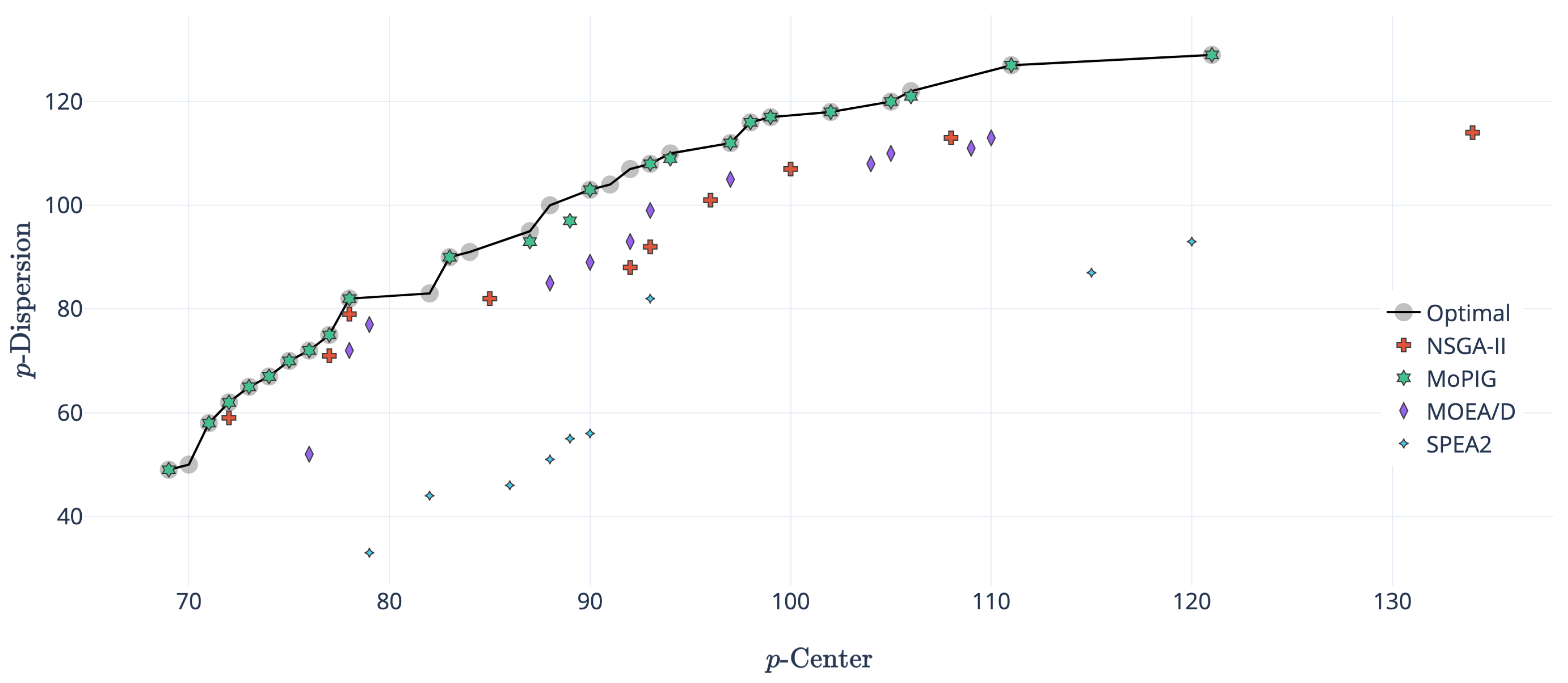
With the aim of graphically analyzing the differences between both algorithms, the approximation front obtained by MoPIG, NSGA-II, MOEA/D, SPEA2, and the $ϵ$-constraint of three representative instances are depicted.

Figure 3 shows an example of an instance where MoPIG was able to reach the optimal Pareto front. As can be seen in the figure, MOEA/D was able to reach a near-optimal approximation front, but there were some solutions that were covered by the optimal front (those located under the curve of the optimal front). The approximation front of NSGA-II was close to the one provided by MOEA/D, but reaching a smaller number of solutions of the Pareto front. Finally, SPEA2 was the worst performing algorithm, being unable to reach any solution of the optimal front.

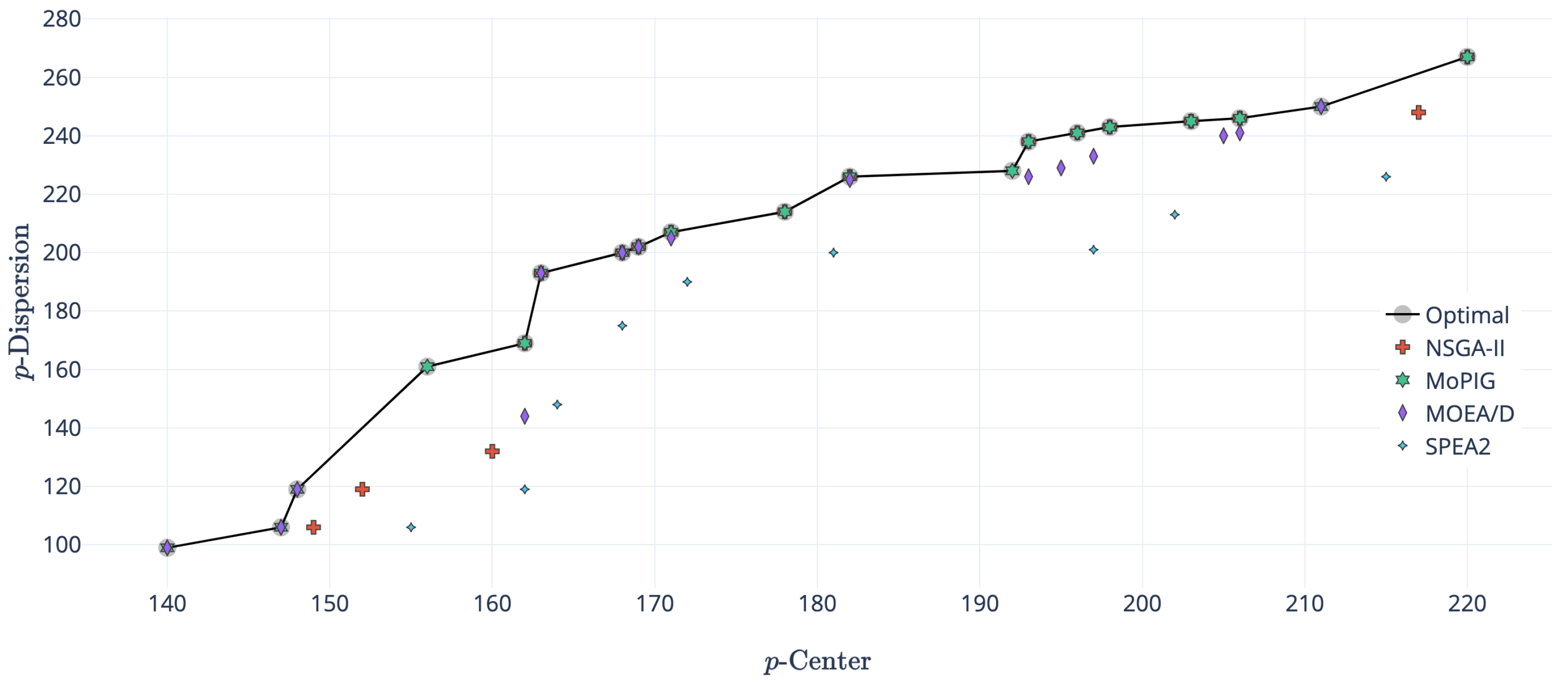
On the contrary, Figure 4 shows an example in which the complete optimal front was not reached by any of the algorithms. However, the figure shows how MoPIG missed only seven solutions, staying pretty close to two of them. On the contrary, neither MOEA/D nor NSGA-II were able to reach any solution of the optimal front, but staying reasonably close to it. Again, the approximation front of SPEA2 was far away from the Pareto front.

Finally, Figure 5 shows one of those instance where the optimal front was hard to find for all the compared algorithms. Even in this case, MoPIG was able to find an approximation front very similar to the optimal one. Although MOEA/D showed its superiority with respect to both NSGA-II and SPEA2, its front was completely dominated by the optimal one.

Having analyzed these results, MoPIG emerged as the most competitive heuristic algorithm for solving $BpCD$, balancing the quality of the solutions obtained and the computing time required for solving them.

5. Conclusions

The Bi-objective p-Center p-Dispersion problem ($BpCD$) seeks to minimize the maximum distance between facilities and demand points and, at the same time, to maximize the minimum distance between all pairs of facilities. Many real-world applications fit in this model since the majority of realistic situations cannot be addressed as single-objective location problems since the decision maker is usually interested in more than one criterion at the same time to locate facilities.

To address this problem, a Multi-objective Parallel Iterated Greedy (MoPIG) was specifically designed for the solution of $BpCD$. This algorithm was able to find the approximation front in short computing times, emerging as a competitive algorithm from a heuristic point of view in the state-of-the art. Computational experiments showed the effectiveness of our proposed algorithm for solving relatively large instances of this bi-criteria optimization problem, requiring half of the time of the MOEA/D, NSGA-II, and SPEA2 genetic algorithms and obtaining better approximation fronts. In particular, the front obtained with MoPIG was really close to the optimal one (with a percentage of dominated solutions by the optimal front smaller than 25%), while the front provided by genetic algorithms was covered in more than 75% of the solutions.

As future research, it would be interesting to test this adaptation of the iterated greedy to the multi-criteria optimization by applying it to a diverse set of multi-objective optimization problems in order to evaluate the effort of designing new algorithms based on this framework.

References

1. Chauhan, D.; Unnikrishnan, A.; Figliozzi, M. Maximum coverage capacitated facility location problem with range constrained drones. Transp. Res. Part C 2019, 99, 1–18. [Google Scholar] [CrossRef]
2. Kung, L.C.; Liao, W.H. An approximation algorithm for a competitive facility location problem with network effects. Eur. J. Oper. Res. 2018, 267, 176–186. [Google Scholar] [CrossRef]
3. Ahmadi-Javid, A.; Seyedi, P.; Syam, S.S. A survey of healthcare facility location. Comput. Oper. Res. 2017, 79, 223–263. [Google Scholar] [CrossRef]
4. Erkut, E. The discrete p-dispersion problem. Eur. J. Oper. Res. 1990, 46, 48–60. [Google Scholar] [CrossRef]
5. Sayah, D.; Irnich, S. A new compact formulation for the discrete p-dispersion problem. Eur. J. Oper. Res. 2017, 256, 62–67. [Google Scholar] [CrossRef]
6. Minieka, E. The m-center problem. Siam Rev. 1970, 12, 138–139. [Google Scholar] [CrossRef]
7. Contardo, C.; Iori, M.; Kramer, R. A scalable exact algorithm for the vertex p-center problem. Comput. Oper. Res. 2019, 103, 211–220. [Google Scholar] [CrossRef]
8. Albareda-Sambola, M.; Hinojosa, Y.; Marín, A.; Puerto, J. When centers can fail: A close second opportunity. Comput. Oper. Res. 2015, 62, 145–156. [Google Scholar] [CrossRef]
9. López-Sánchez, A.D.; Sánchez-Oro, J.; Hernández-Díaz, A.G. GRASP and VNS for solving the p-next center problem. Comput. Oper. Res. 2019, 104, 295–303. [Google Scholar] [CrossRef]
10. Kariv, O.; Hakimi, S.L. An Algorithmic Approach to Network Location Problems. I: The p-Centers. SIAM J. Appl. Math. 1979, 37, 513–538. [Google Scholar] [CrossRef]
11. Colmenar, J.; Martí, R.; Duarte, A. Multi-objective memetic optimization for the bi-objective obnoxious p-median problem. Knowl.-Based Syst. 2018, 144, 88–101. [Google Scholar] [CrossRef]
12. Colmenar, J.M.; Hoff, A.; Martí, R.; Duarte, A. Scatter search for the bi-criteria p-median p-dispersion problem. Prog. Artif. Intell. 2018, 7, 31–40. [Google Scholar] [CrossRef]
13. Zhang, W.; Cao, K.; Liu, S.; Huang, B. A multi-objective optimization approach for health-care facility location-allocation problems in highly developed cities such as Hong Kong. Comput. Environ. Urban Syst. 2016, 59, 220–230. [Google Scholar] [CrossRef]
14. Badri, M.A.; Mortagy, A.K.; Alsayed, C.A. A multi-objective model for locating fire stations. Eur. J. Oper. Res. 1998, 110, 243–260. [Google Scholar] [CrossRef]
15. Stummer, C.; Doerner, K.; Focke, A.; Heidenberger, K. Determining location and size of medical departments in a hospital network: A multiobjective decision support approach. Health Care Manag. Sci. 2004, 7, 63–71. [Google Scholar] [CrossRef]
16. Drezner, T.; Drezner, Z.; Salhi, S. A multi-objective heuristic approach for the casualty collection points location problem. J. Oper. Res. Soc. 2006, 57, 727–734. [Google Scholar] [CrossRef]
17. Gortázar, F.; Duarte, A.; Laguna, M.; Martí, R. Black box scatter search for general classes of binary optimization problems. Comput. Oper. Res. 2010, 37, 1977–1986. [Google Scholar] [CrossRef]
18. Laguna, M.; Gortázar, F.; Gallego, M.; Duarte, A.; Martí, R. A black-box scatter search for optimization problems with integer variables. J. Glob. Optim. 2014, 58, 497–516. [Google Scholar] [CrossRef]
19. Daskin, M.S. Network and Discrete Location; John Wiley & Sons, Inc.: Hoboken, NJ, USA, 1995. [Google Scholar]
20. Mladenović, N.; Labbé, M.; Hansen, P. Solving the p-center problem with tabu search and variable neighborhood search. Networks 2003, 42, 48–64. [Google Scholar] [CrossRef]
21. Davidovic, T.; Ramljak, D.; Selmic, M.; Teodorovic, D. Bee colony optimization for the p-center problem. Comput. Oper. Res. 2011, 38, 1367–1376. [Google Scholar] [CrossRef]
22. Sayyady, F.; Fathi, Y. An integer programming approach for solving the p-dispersion problem. Eur. J. Oper. Res. 2016, 253, 216–225. [Google Scholar] [CrossRef]
23. Tutunchi, G.K.; Fathi, Y. Effective methods for solving the Bi-criteria p-Center and p-Dispersion problem. Comput. Oper. Res. 2019, 101, 43–54. [Google Scholar] [CrossRef]
24. Ruiz, R.; Stützle, T. A simple and effective iterated greedy algorithm for the permutation flow shop scheduling problem. Eur. J. Oper. Res. 2007, 177, 2033–2049. [Google Scholar] [CrossRef]
25. Pranzo, M.; Pacciarelli, D. An iterated greedy metaheuristic for the blocking job shop scheduling problem. J. Heuristics 2016, 22, 587–611. [Google Scholar] [CrossRef]
26. Ruiz, R.; Pan, Q.K.; Naderi, B. Iterated Greedy methods for the distributed permutation flow shop scheduling problem. Omega 2019, 83, 213–222. [Google Scholar] [CrossRef]
27. Sánchez-Oro, J.; Duarte, A. Iterated Greedy algorithm for performing community detection in social networks. Future Gener. Comput. Syst. 2018, 88, 785–791. [Google Scholar] [CrossRef]
28. Framinan, J.M.; Leisten, R. A multi-objective iterated greedy search for flow shop scheduling with makespan and flowtime criteria. OR Spectr. 2008, 30, 787–804. [Google Scholar] [CrossRef]
29. Minella, G.; Ruiz, R.; Ciavotta, M. Restarted Iterated Pareto Greedy algorithm for multi-objective flow shop scheduling problems. Comput. Oper. Res. 2011, 38, 1521–1533. [Google Scholar] [CrossRef]
30. Duarte, A.; Pantrigo, J.J.; Pardo, E.G.; Mladenovic, N. Multi-objective variable neighborhood search: an application to combinatorial optimization problems. J. Glob. Optim. 2015, 63, 515–536. [Google Scholar] [CrossRef]
31. Sánchez-Oro, J.; Pantrigo, J.J.; Duarte, A. Combining intensification and diversification strategies in VNS. An application to the Vertex Separation problem. Comput. Oper. Res. 2014, 52, 209–219. [Google Scholar] [CrossRef]
32. Sánchez-Oro, J.; Mladenović, N.; Duarte, A. General Variable Neighborhood Search for computing graph separators. Optim. Lett. 2017, 11, 1069–1089. [Google Scholar] [CrossRef]
33. Feo, T.A.; Resende, M.G.C.; Smith, S.H. A Greedy Randomized Adaptive Search Procedure for Maximum Independent Set. Oper. Res. 1994, 42, 860–878. [Google Scholar] [CrossRef]
34. Beasley, J.E. OR-Library: Distributing Test Problems by Electronic Mail. J. Oper. Res. Soc. 1990, 41, 1069–1072. [Google Scholar] [CrossRef]
35. Li, M.; Yao, X. Quality evaluation of solution sets in multiobjective optimisation: A survey. ACM Comput. Surv. (CSUR) 2019, 52, 26. [Google Scholar] [CrossRef]
36. Redondo, J.L.; Fernández, J.; Hervás, J.D.Á.; Arrondo, A.G.; Ortigosa, P.M. Approximating the Pareto-front of a planar bi-objective competitive facility location and design problem. Comput. Oper. Res. 2015, 62, 337–349. [Google Scholar] [CrossRef]
37. Bhattacharya, R.; Bandyopadhyay, S. Solving conflicting bi-objective facility location problem by NSGA II evolutionary algorithm. Int. J. Adv. Manuf. Technol. 2010, 51, 397–414. [Google Scholar] [CrossRef]
38. Pangilinan, J.M.A.; Janssens, G.K.; Caris, A. Sensitivity analysis of a genetic algorithm for a competitive facility location problem. In Innovations and Advanced Techniques in Systems, Computing Sciences and Software Engineering; Springer: Dordrecht, The Netherlands, 2008; pp. 266–271. [Google Scholar]
39. Zhang, Q.; Li, H. MOEA/D: A multiobjective evolutionary algorithm based on decomposition. IEEE Trans. Evolut. Comput. 2007, 11, 712–731. [Google Scholar] [CrossRef]
40. Kumari, R.; Kumar, D.; Kumar, V. A conceptual comparison of NSGA-II, OMOPSO and AbYss algorithms. Int. J. Internet Technol. Secur. Trans. 2017, 7, 330–352. [Google Scholar] [CrossRef]
41. Zitzler, E.; Laumanns, M.; Thiele, L. SPEA2: Improving the Strength Pareto Evolutionary Algorithm. EUROGEN 2001, 2002, 95–100. [Google Scholar]
Figure 1. ( f p C , f p D ) = ( 1.44 , 2.24 ) .
Electronics 08 01440 g001
Figure 2. ( f p C , f p D ) = ( 2.00 , 3.00 ) .
Electronics 08 01440 g002
Figure 3. Sets of non-dominated solutions obtained by NSGA-II, ϵ -constraint, SPEA2, MOEA/D, and MoPIG for instance pmed4, with n = 80 and p = 5 .
Electronics 08 01440 g003
Figure 4. Sets of non-dominated solutions obtained by NSGA-II, ϵ -constraint, SPEA2, MOEA/D, and MoPIG for instance pmed7, with n = 150 and p = 10 .
Electronics 08 01440 g004
Figure 5. Sets of non-dominated solutions obtained by NSGA-II, ϵ -constraint, SPEA2, MOEA/D, and MoPIG for instance pmed8, with n = 150 and p = 10 .
Electronics 08 01440 g005