Optimal Robot Motion Planning of Redundant Robots in Machining and Additive Manufacturing Applications

 , , ,
, , ,  ,
,  and
and
Abstract
:1. Introduction
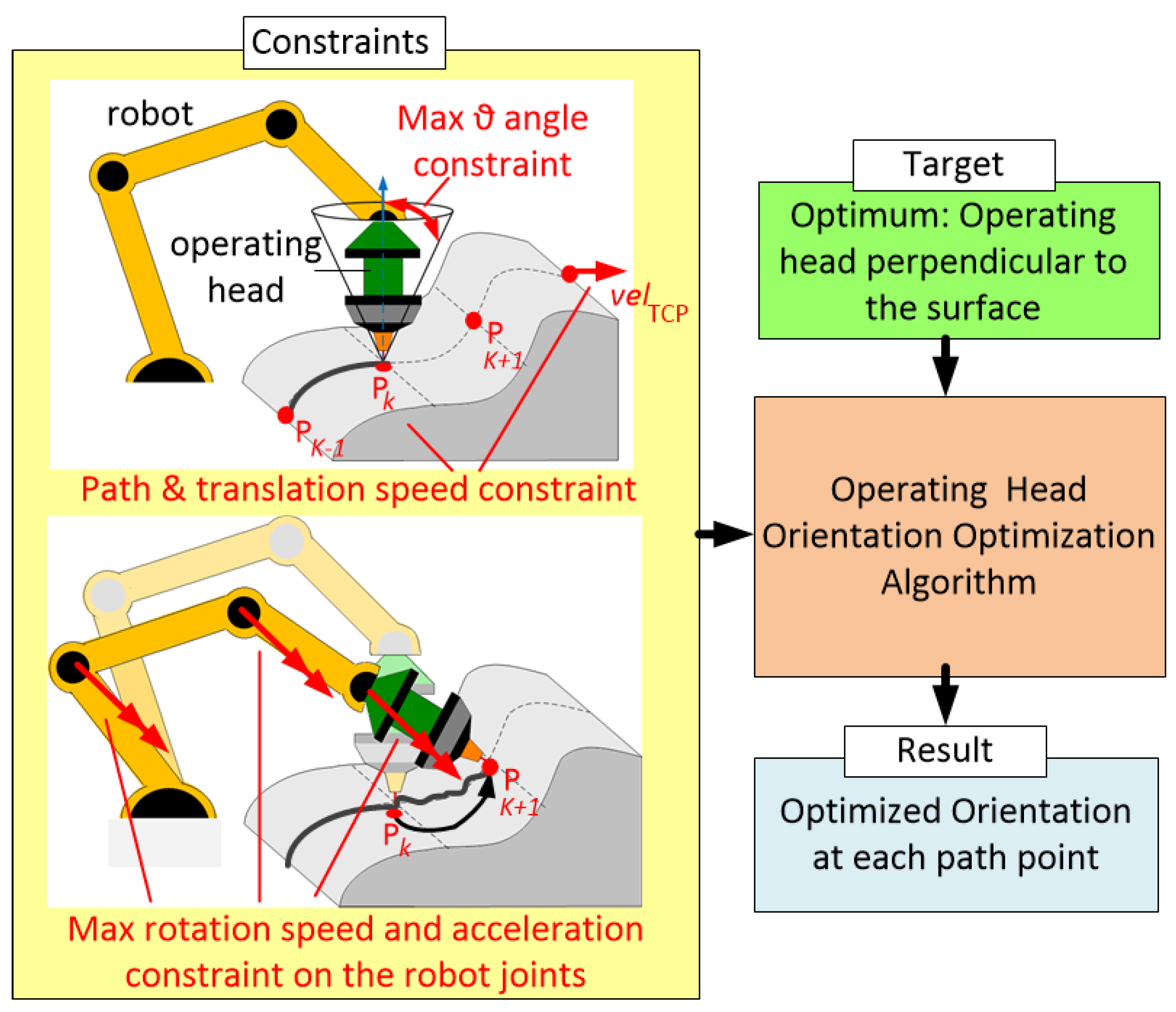
2. Technological Trajectories And Constraints
3. Proposed Framework for Task Formalization
4. Examples of Common Technological Tasks
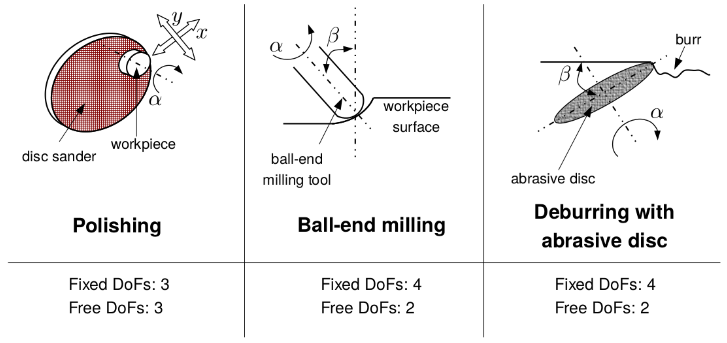
4.1. 5-DoF Tasks
4.2. 3-DoF Tasks
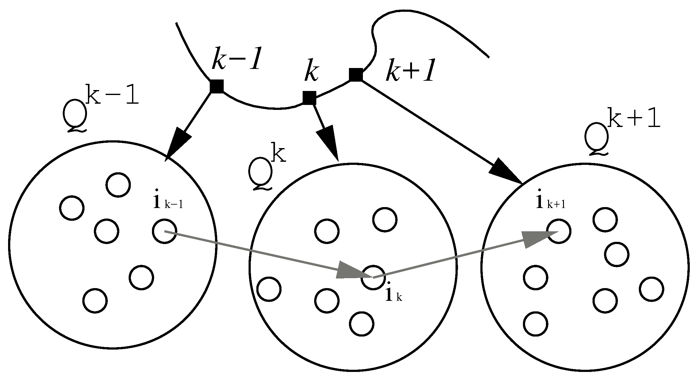
5. Ant Colony Optimization Algorithm
- Set is discretized into set , sampling in redundancy subspace;
- Set is obtained by solving the inverse kinematic problem for all elements of ;
- The pheromone value of each vertex is initialized equal to ;
- Each ant randomly selects the next vertex based on the transition probability Equation (19);
- Ants are ranked based on the path cost;
- m best ants are selected, collision checking is performed on the vertexes which are selected the first time. If an ant path is in collision, this ant is replaced by the next ant in the ranking;
- The best solution found since the beginning of the whole optimization is added to the set of the best ants found at the current iteration;
- The best ants update the pheromone values of the vertexes of their path by adding a quantity that is inversely proportional to the cost function of its entire network path, that is:
- The pheromone evaporation is performed for all the vertexes
- If termination conditions are not satisfied, go to step 4.
6. Case Studies
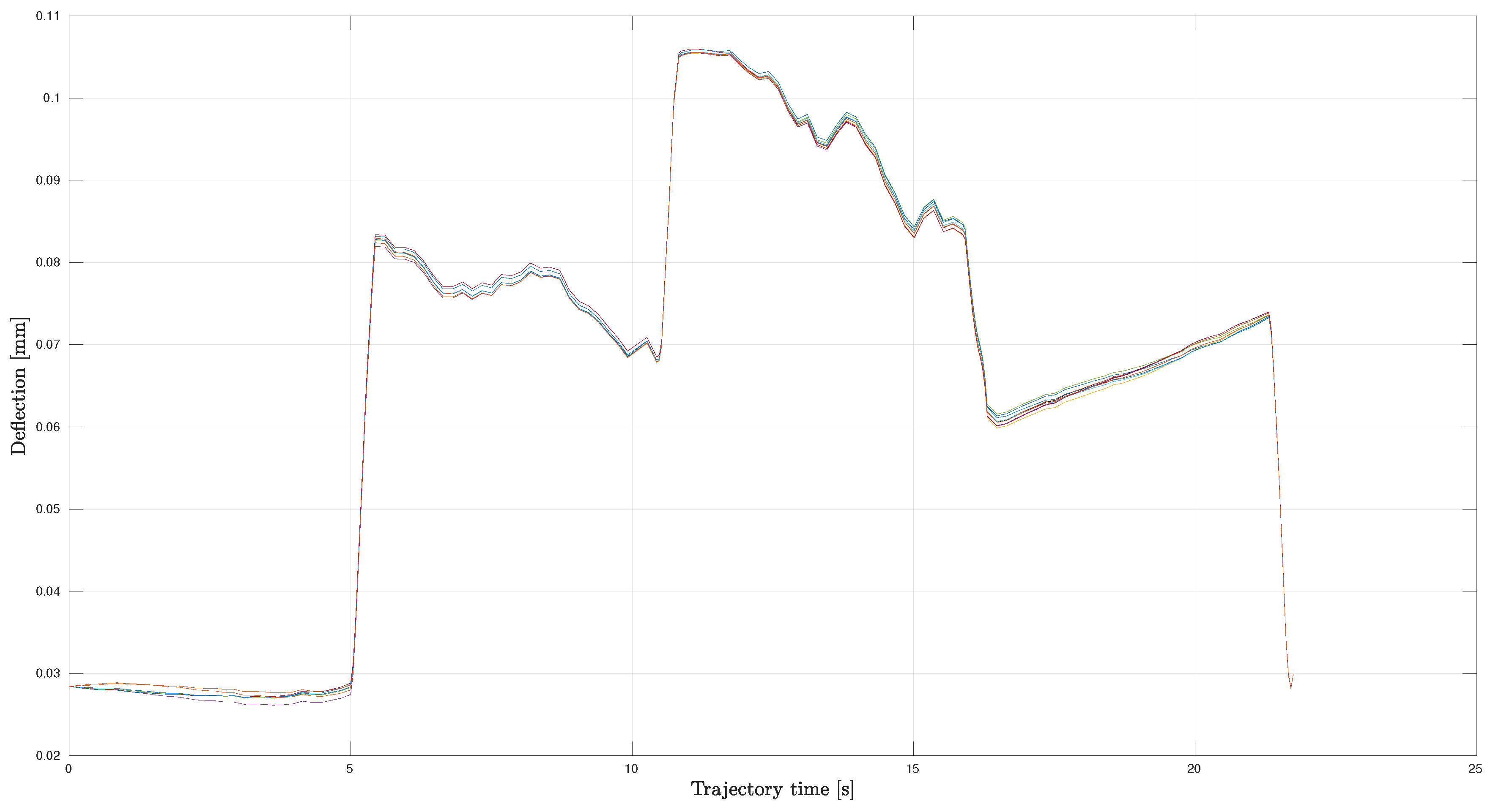
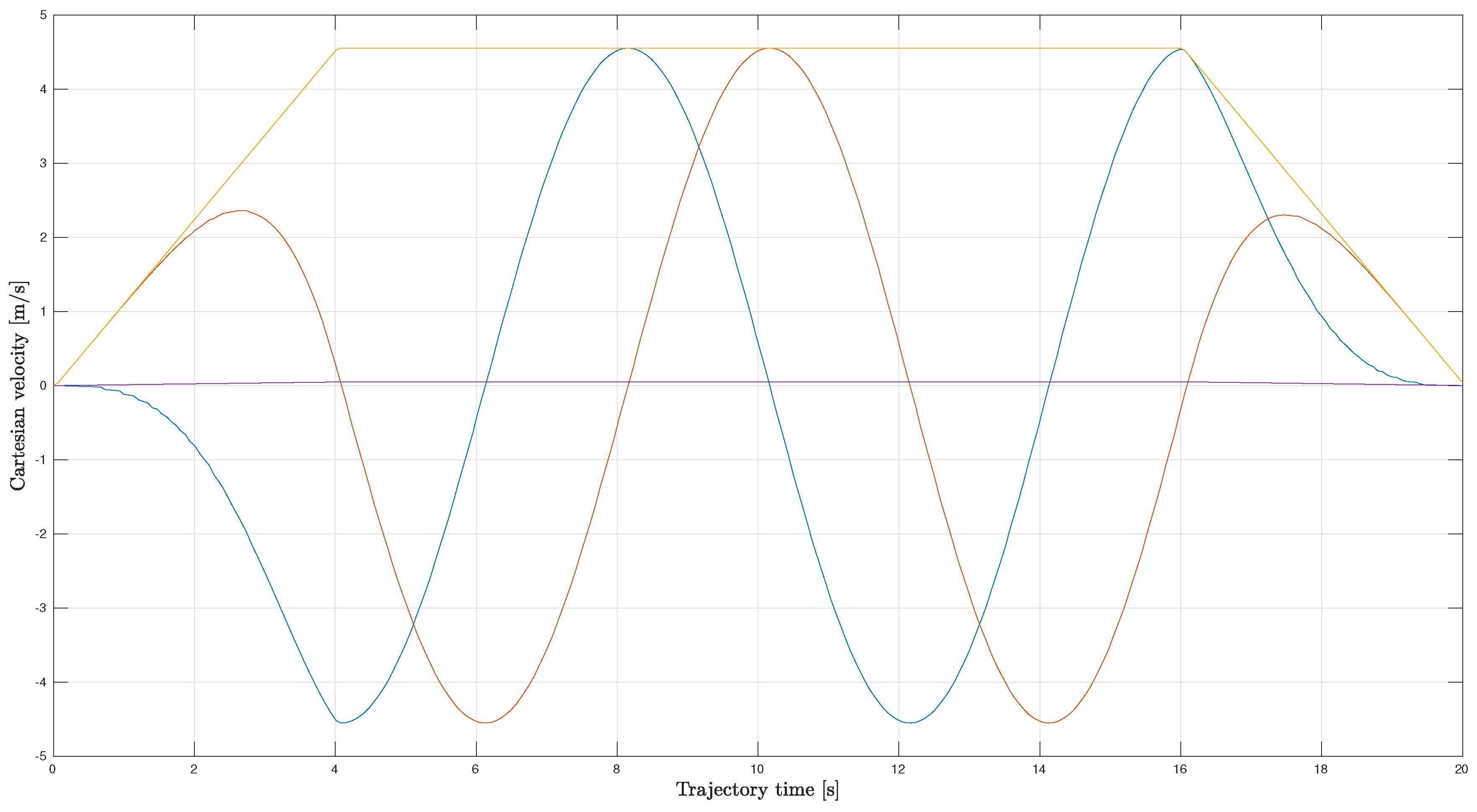
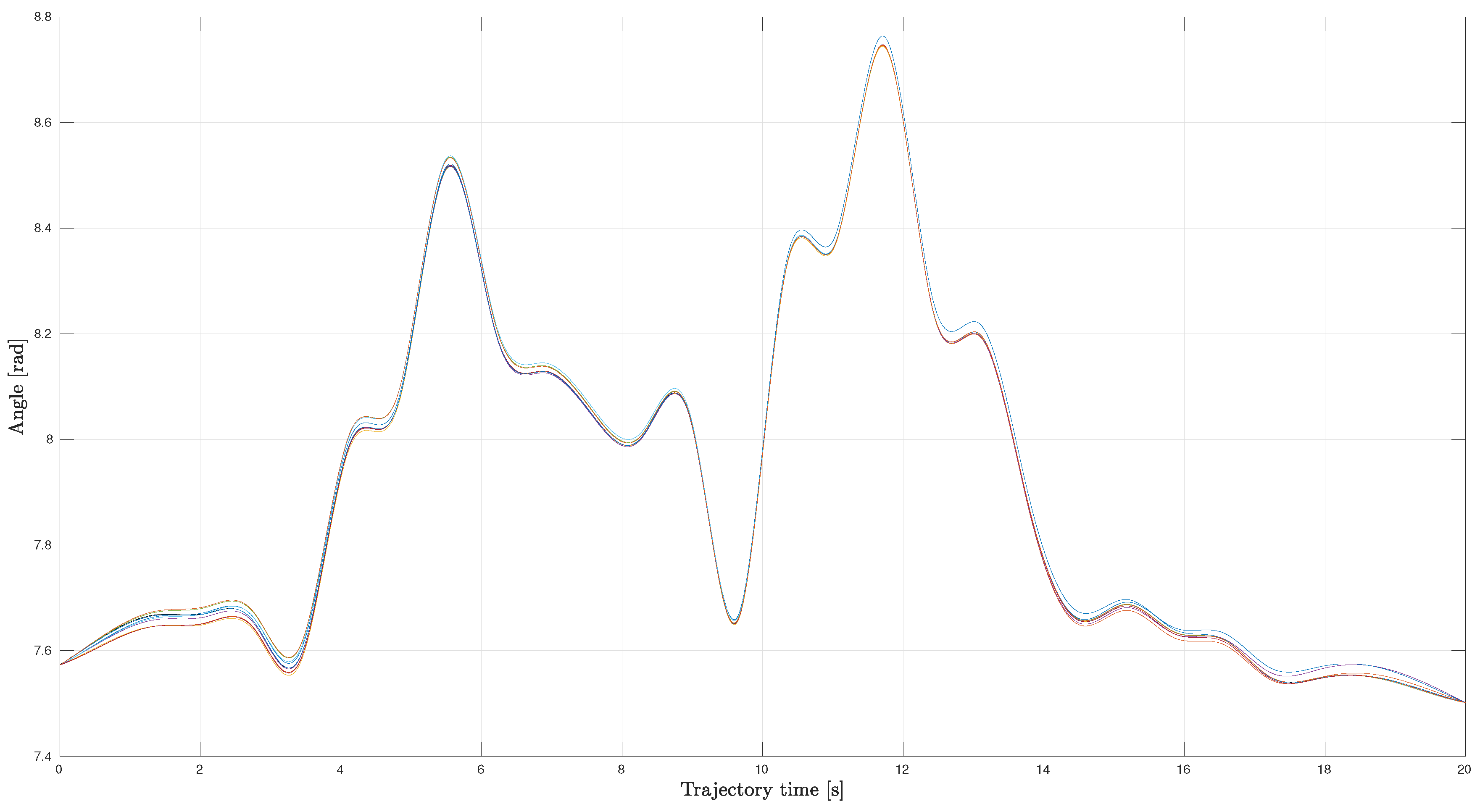
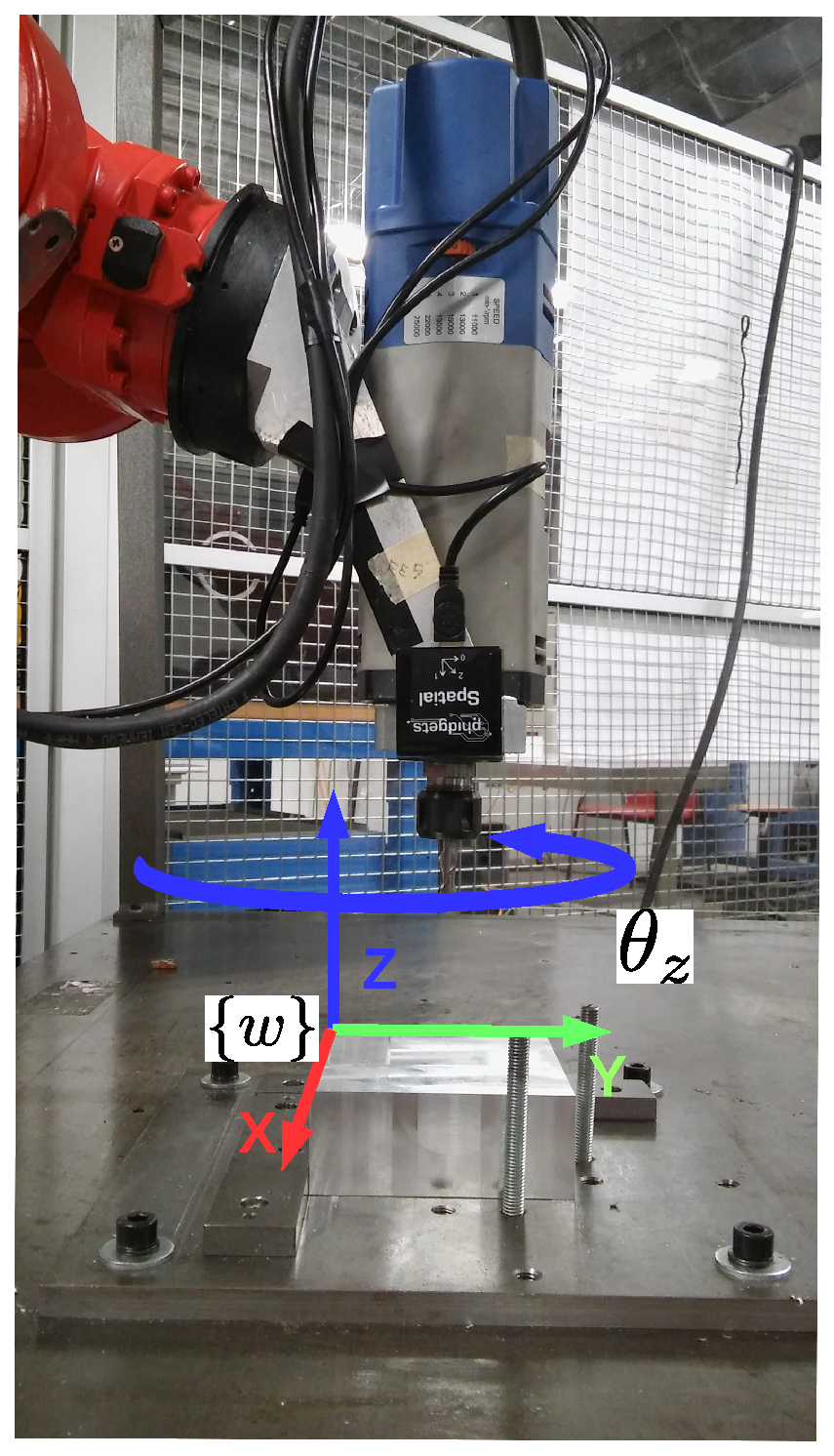
6.1. Milling Task
- a standard Ant Colony Optimization solver (denoted as ACO) [38];
- a rank-based Ant Colony approach (denoted as RB) [40];
- a Ant Colony approach (denoted as MM) [41];
- a local solver (denoted as LS) where is selected as the vertex with minimum cost in and, for each step k, the next vertex is selected as the vertex with minimum cost in which can be reached from with a feasible transition.
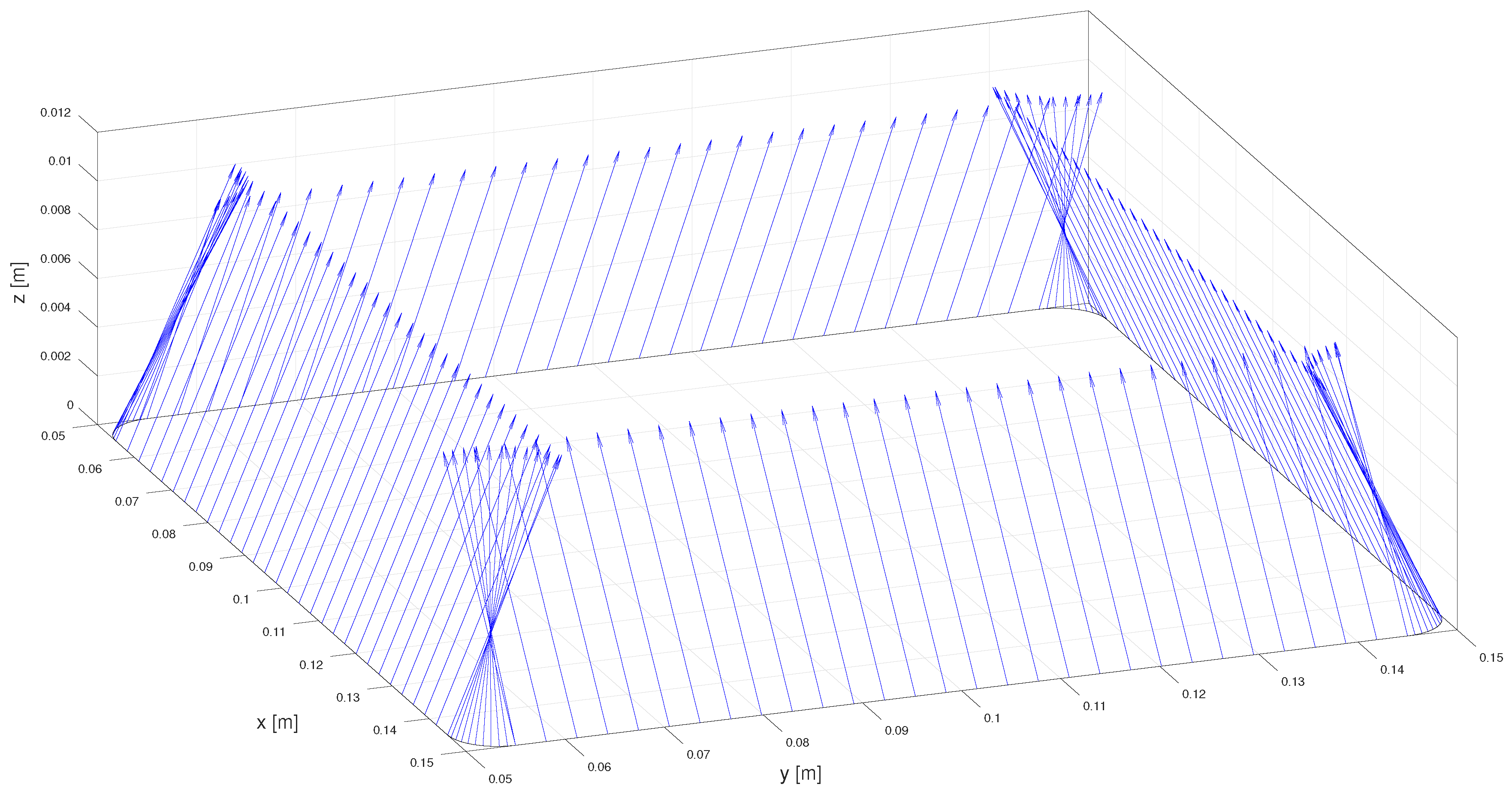
6.2. Additive Manufacturing
7. Conclusions
Author Contributions
Funding
Conflicts of Interest
Abbreviations
| n | number of degrees of freedom of the robot |
| q | joint configuration vector |
| joint velocity vector | |
| joint acceleration vector | |
| joint effort vector | |
| transformation matrix from frame b to frame a | |
| origin of frame b in frame a | |
| linear velocity of the origin of frame b in frame a | |
| angular velocity of frame b in frame a | |
| linear acceleration of the origin of frame b in frame a | |
| angular acceleration of frame b in frame a | |
| velocity twist vector from frame b to frame a, defined as | |
| acceleration twist vector from frame b to frame a, defined as | |
| transformation matrix from robot end-effector frame to workpiece frame w | |
| transformation matrix from CAM output frame to workpiece frame w at trajectory sample k | |
| N | number of samples of the desired trajectory |
| - | is the forward kinematic function of the robot; |
| - | is the velocity forward kinematic function; |
| - | is the acceleration forward kinematic function; |
| - | is the inverse dynamics function; |
| - | is the collision function, which is equal to 1 in case of one or more collisions, 0 otherwise. |
| - | admissible joint configuration set where and are, respectively, the lower and upper joint limits; |
| - | admissible joint velocities set where and are, respectively, the lower and upper joint velocity limits; |
| - | admissible joint effort set where and are, respectively, the lower and upper joint effort limits; |
| - | admissible Cartesian velocities set where , , , and are, respectively, the lower and upper linear and angular velocity limits. |
References
- Mohanan, M.; Salgoankar, A. A survey of robotic motion planning in dynamic environments. Robot. Auton. Syst. 2018, 100, 171–185. [Google Scholar] [CrossRef]
- Erdos, G.; Kovács, A.; Váncza, J. Optimized joint motion planning for redundant industrial robots. CIRP Ann. Manuf. Technol. 2016, 65, 451–454. [Google Scholar] [CrossRef]
- LaValle, S.M. Planning Algorithms; Cambridge University Press: Cambridge, UK, 2006. [Google Scholar]
- Jaillet, L.; Cortés, J.; Siméon, T. Sampling-Based Path Planning on Configuration-Space Costmaps. IEEE Trans. Robot. 2010, 26, 635–646. [Google Scholar] [CrossRef]
- Devaurs, D.; Simeon, T.; Cortes, J. Enhancing the transition-based RRT to deal with complex cost spaces. In Proceedings of the IEEE International Conference on Robotics and Automation, Karlsruhe, Germany, 17 October 2013; pp. 4120–4125. [Google Scholar] [CrossRef]
- Adiyatov, O.; Varol, H.A. A novel RRT*-based algorithm for motion planning in Dynamic environments. In Proceedings of the IEEE International Conference on Mechatronics and Automation, Takamatsu, Japan, 6–9 August 2017; pp. 1416–1421. [Google Scholar] [CrossRef]
- Choudhury, S.; Gammell, J.D.; Barfoot, T.D.; Srinivasa, S.S.; Scherer, S. Regionally accelerated batch informed trees (RABIT*): A framework to integrate local information into optimal path planning. In Proceedings of the IEEE International Conference on Robotics and Automation, Stockholm, Sweden, 16–21 May 2016; pp. 4207–4214. [Google Scholar] [CrossRef]
- Gammell, J.D.; Srinivasa, S.S.; Barfoot, T.D. Informed RRT*: Optimal sampling-based path planning focused via direct sampling of an admissible ellipsoidal heuristic. In Proceedings of the IEEE/RSJ International Conference on Intelligent Robots and Systems, Chicago, IL, USA, 14–18 September 2014; pp. 2997–3004. [Google Scholar] [CrossRef]
- Salzman, O.; Halperin, D. Asymptotically-optimal Motion Planning using lower bounds on cost. In Proceedings of the IEEE International Conference on Robotics and Automation, Seattle, WA, USA, 26–30 May 2015; pp. 4167–4172. [Google Scholar] [CrossRef]
- Schulman, J.; Ho, J.; Lee, A.; Awwal, I.; Bradlow, H.; Abbeel, P. Finding locally optimal, collision-free trajectories with sequential convex optimization. In Proceedings of the Robotics: Science and Systems, Berlin, Germany, 24–28 June 2013. [Google Scholar] [CrossRef]
- Kunz, T.; Stilman, M. Time-optimal trajectory generation for path following with bounded acceleration and velocity. In Robotics: Science and Systems; MIT Press: Cambridge, MA, USA, 2013; Volume 8, pp. 209–216. [Google Scholar]
- Faroni, M.; Beschi, M.; Pedrocchi, N.; Visioli, A. Predictive Inverse Kinematics for Redundant Manipulators with Task Scaling and Kinematic Constraints. IEEE Trans. Robot. 2019, 35, 278–285. [Google Scholar] [CrossRef]
- Zucker, M.; Ratliff, N.; Dragan, A.D.; Pivtoraiko, M.; Klingensmith, M.; Dellin, C.M.; Bagnell, J.A.; Srinivasa, S.S. CHOMP: Covariant Hamiltonian optimization for motion planning. Int. J. Robot. Res. 2013, 32, 1164–1193. [Google Scholar] [CrossRef]
- Kalakrishnan, M.; Chitta, S.; Theodorou, E.; Pastor, P.; Schaal, S. STOMP: Stochastic trajectory optimization for motion planning. In Proceedings of the IEEE International Conference on Robotics and Automation, Shanghai, China, 9–13 May 2011. [Google Scholar] [CrossRef]
- Donald, B.; Xavier, P.; Canny, J.; Reif, J. Kinodynamic motion planning. J. ACM 1993, 40, 1048–1066. [Google Scholar] [CrossRef]
- Kingston, Z.; Moll, M.; Kavraki, L.E. Sampling-based methods for motion planning with constraints. Annu. Rev. Control. Robot. Auton. Syst. 2018, 1, 159–185. [Google Scholar] [CrossRef]
- Kingston, Z.; Moll, M.; Kavraki, L.E. Exploring implicit spaces for constrained sampling-based planning. Int. J. Robot. Res. 2019, 38, 1151–1178. [Google Scholar] [CrossRef]
- Sabourin, L.; Subrin, K.; Cousturier, R.; Gogu, G.; Mezouar, Y. Redundancy-based optimization approach to optimize robotic cell behaviour: Application to robotic machining. Ind. Robot. 2015, 42, 167–178. [Google Scholar] [CrossRef]
- Fang, H.; Ong, S.; Nee, A. Robot path planning optimization for welding complex joints. Int. J. Adv. Manuf. Technol. 2017, 90, 3829–3839. [Google Scholar] [CrossRef]
- Shahabi, M.; Ghariblu, H.; Beschi, M. Obstacle avoidance of redundant robotic manipulators using safety ring concept. Int. J. Comput. Integr. Manuf. 2019, 32, 695–704. [Google Scholar] [CrossRef]
- Magnoni, P.; Pedrocchi, N.; Thieme, S.; Legnani, G.; Tosatti, L.M. Optimal planning in robotized cladding processes on generic surfaces. Robotica 2018. [Google Scholar] [CrossRef]
- Iglesias, I.; Sebastián, M.; Ares, J. Overview of the State of Robotic Machining: Current Situation and Future Potential. Procedia Eng. 2015, 132, 911–917. [Google Scholar] [CrossRef]
- Sadílek, M.; Čep, R.; Budak, I.; Soković, M. Aspects of using tool axis inclination angle. Stroj. Vestnik/J. Mech. Eng. 2011, 57, 681–688. [Google Scholar] [CrossRef]
- Nowotny, S.; Scharek, S.; Beyer, E.; Richter, K. Laser beam build-up welding: Precision in repair, surface cladding, and direct 3D metal deposition. J. Therm. Spray Technol. 2007, 16, 344–348. [Google Scholar] [CrossRef]
- Gao, J.; Chen, X.; Yilmaz, O.; Gindy, N. An integrated adaptive repair solution for complex aerospace components through geometry reconstruction. Int. J. Adv. Manuf. Technol. 2008, 36, 1170–1179. [Google Scholar] [CrossRef]
- Denkena, B.; Boess, V.; Nespor, D.; Floeter, F.; Rust, F. Engine blade regeneration: A literature review on common technologies in terms of machining. Int. J. Adv. Manuf. Technol. 2015, 81, 917–924. [Google Scholar] [CrossRef]
- Calleja, A.; Tabernero, I.; Fernández, A.; Celaya, A.; Lamikiz, A.; de Lacalle, L.L. Improvement of strategies and parameters for multi-axis laser cladding operations. Opt. Lasers Eng. 2014, 56, 113–120. [Google Scholar] [CrossRef]
- Lalas, C.; Tsirbas, K.; Salonitis, K.; Chryssolouris, G. An analytical model of the laser clad geometry. Int. J. Adv. Manuf. Technol. 2007, 32, 34–41. [Google Scholar] [CrossRef]
- Liu, J.; Li, L. In-time motion adjustment in laser cladding manufacturing process for improving dimensional accuracy and surface finish of the formed part. Opt. Laser Technol. 2004, 36, 477–483. [Google Scholar] [CrossRef]
- Xu, M.; Li, J.; Jiang, J.; Li, B. Influence of Powders and Process Parameters on Bonding Shear Strength and Micro Hardness in Laser Cladding Remanufacturing. Procedia CIRP 2015, 29, 804–809. [Google Scholar] [CrossRef]
- Pastras, G.; Fysikopoulos, A.; Chryssolouris, G. A theoretical investigation on the potential energy savings by optimization of the robotic motion profiles. Robot. Comput. Integr. Manuf. 2019. [Google Scholar] [CrossRef]
- Latombe, J.C. Robot Motion Planning; Kluwer Academic Publishers: Boston, MA, USA, 1991. [Google Scholar]
- Chen, C.; Hu, S.; He, D.; Shen, J. An approach to the path planning of tube-sphere intersection welds with the robot dedicated to J-groove joints. Robot. Comput. Integr. Manuf. 2013, 29, 41–48. [Google Scholar] [CrossRef]
- Léger, J.; Angeles, J. Off-line programming of six-axis robots for optimum five-dimensional tasks. Mech. Mach. Theory 2016, 100, 155–169. [Google Scholar] [CrossRef]
- Subrin, K.; Sabourin, L.; Gogu, G.; Mezouar, Y. Intrinsic redundancy to optimize the robotic cell behavior: Application to robotic machining. In Proceedings of the 21ème Congrès Français de Mécanique, Bordeaux, France, 26–30 August 2013; pp. 2–7. [Google Scholar]
- Lasemi, A.; Xue, D.; Gu, P. Recent development in CNC machining of freeform surfaces: A state-of-the-art review. Comput. Aided Des. 2010, 42, 641–654. [Google Scholar] [CrossRef]
- Sellmann, F.; Haas, T.; Nguyen, H.; Weikert, S.; Wegener, K. Orientation smoothing for 5-axis machining using quasi-redundant degrees of freedom. Int. J. Autom. Technol. 2016, 10, 262–271. [Google Scholar] [CrossRef]
- Dorigo, M.; Birattari, M.; Stutzle, T. Ant colony optimization. IEEE Comput. Intell. Mag. 2006, 1, 28–39. [Google Scholar] [CrossRef]
- Chandra Mohan, B.; Baskaran, R. A survey: Ant Colony Optimization based recent research and implementation on several engineering domain. Expert Syst. Appl. 2012, 39, 4618–4627. [Google Scholar] [CrossRef]
- Hartl, R.F. A New Rank Based Version of the Ant System—A Computational Study Bernd Bullnheimer; Institute of Management Science, University of Vienna: Vienna, Austria, 1997. [Google Scholar]
- Stützle, T.; Hoos, H.H. Max-Min Ant System. Future Gener. Comput. Syst. 2000, 16, 889–914. [Google Scholar] [CrossRef]
- Altintas, Y. Manufacturing Automation Metal Cutting Mechanics, Machine Tool Vibrations, and CNC Design; Cambridge University Press: Cambridge, UK, 2012. [Google Scholar]
- Zhang, Z.; Feng, Z.; Ren, Z. Approximate termination condition analysis for ant colony optimization algorithm. In Proceedings of the World Congress on Intelligent Control and Automation, Jinan, China, 23 August 2010; pp. 3211–3215. [Google Scholar] [CrossRef]
- Villagrossi, E. Robot Dynamics Modelling and Control for Machining Applications. Ph.D. Thesis, University of Brescia, Brescia, Italy, December 2016. [Google Scholar]


| b is the axial depth of cut | 1.5 [mm] |
| is the spindle speed | 13,000 [rpm] |
| is the feed velocity | 1080 [mm/min] = 18 [mm/s] |
| arc exit angle | 3.14 [rad] |
| arc enter angle | 1.0472 [rad] |
| is the tangential cutting coefficient | 600 [N/mm] |
| is the radial cutting coefficient | 300 [N/mm] |
| is the tangential edge coefficient | 10 [N/mm] |
| is the radial edge coefficient | 5 [N/mm] |
| is the helix angle | 0.6981 [rad] |
| Method | Cartesian Compliance Index [mm] | Computational Time [s] |
|---|---|---|
| RBMM | 0.0682 ± 0.0019 | 2.21 ± 0.18 |
| ACO [38] | 0.0716 ± 0.0028 | 3.91 ± 1.16 |
| RB [40] | 0.0701 ± 0.0024 | 2.22 ± 0.22 |
| MM [41] | 0.0695 ± 0.0019 | 3.15 ± 0.93 |
| LS | 0.0829 ± 0.0000 | 0.51 ± 0.02 |
| Method | Angle [deg] | Computational Time [s] |
|---|---|---|
| RBMM | 7.902 ± 0.251 | 5.66 ± 0.48 |
| ACO [38] | 8.061 ± 0.378 | 5.91 ± 1.96 |
| RB [40] | 7.924 ± 0.353 | 5.72 ± 0.55 |
| MM [41] | 7.952 ± 0.242 | 8.17 ± 2.93 |
| LS | 8.291 ± 0.000 | 0.91 ± 0.02 |
© 2019 by the authors. Licensee MDPI, Basel, Switzerland. This article is an open access article distributed under the terms and conditions of the Creative Commons Attribution (CC BY) license (http://creativecommons.org/licenses/by/4.0/).
Share and Cite
Beschi, M.; Mutti, S.; Nicola, G.; Faroni, M.; Magnoni, P.; Villagrossi, E.; Pedrocchi, N. Optimal Robot Motion Planning of Redundant Robots in Machining and Additive Manufacturing Applications. Electronics 2019, 8, 1437. https://doi.org/10.3390/electronics8121437
Beschi M, Mutti S, Nicola G, Faroni M, Magnoni P, Villagrossi E, Pedrocchi N. Optimal Robot Motion Planning of Redundant Robots in Machining and Additive Manufacturing Applications. Electronics. 2019; 8(12):1437. https://doi.org/10.3390/electronics8121437
Chicago/Turabian StyleBeschi, Manuel, Stefano Mutti, Giorgio Nicola, Marco Faroni, Paolo Magnoni, Enrico Villagrossi, and Nicola Pedrocchi. 2019. "Optimal Robot Motion Planning of Redundant Robots in Machining and Additive Manufacturing Applications" Electronics 8, no. 12: 1437. https://doi.org/10.3390/electronics8121437
APA StyleBeschi, M., Mutti, S., Nicola, G., Faroni, M., Magnoni, P., Villagrossi, E., & Pedrocchi, N. (2019). Optimal Robot Motion Planning of Redundant Robots in Machining and Additive Manufacturing Applications. Electronics, 8(12), 1437. https://doi.org/10.3390/electronics8121437