Research on the Control Algorithm of Coaxial Rotor Aircraft based on Sliding Mode and PID


Abstract
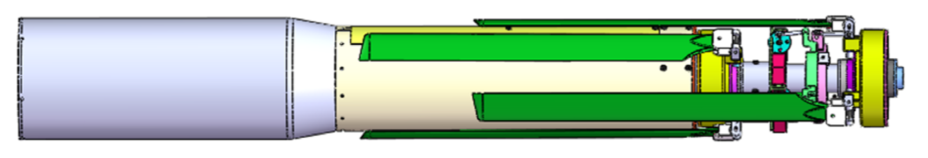
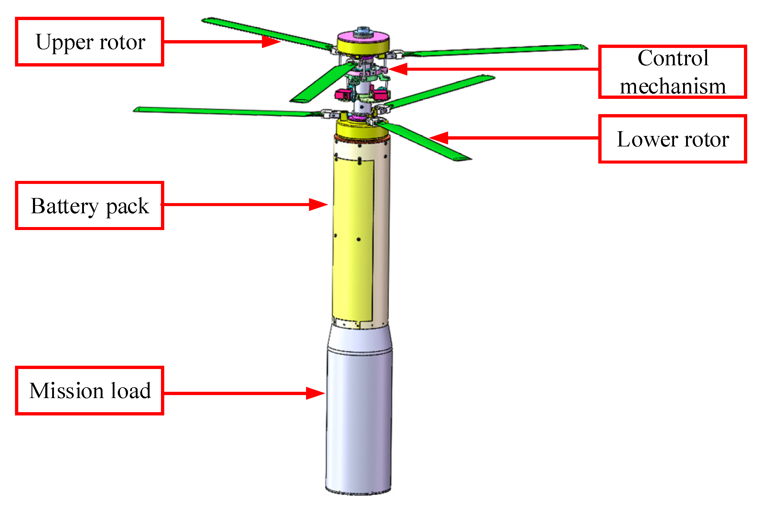
:1. Introduction
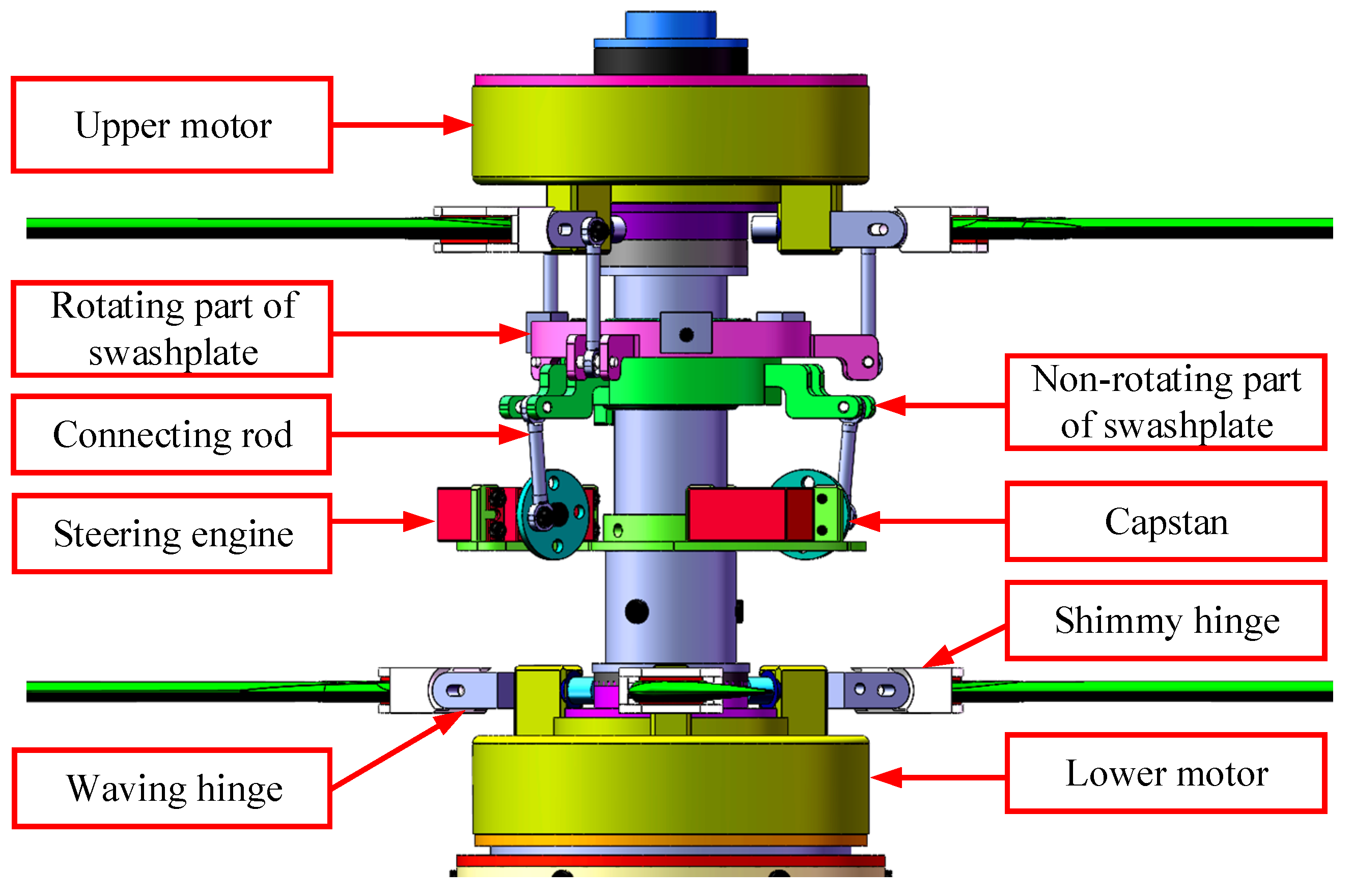
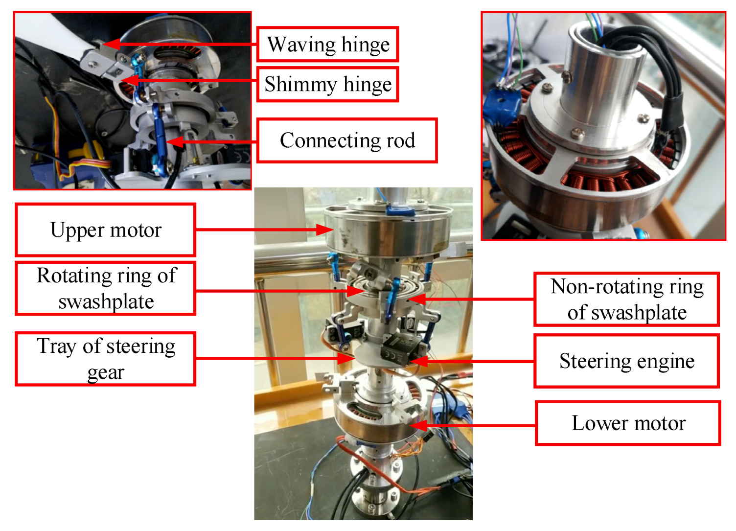
2. Flight Control Principle
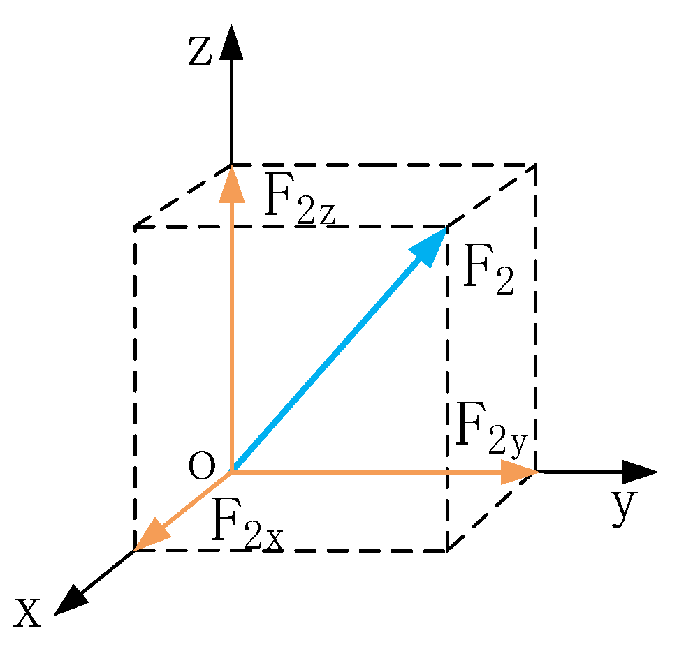
3. Aircraft Kinetic Model
3.1. Model without Rotor Interference or Flapping Motion
- (1)
- The whole coaxial rotor aircraft is regarded as a rigid body.
- (2)
- The centroid of the coaxial rotor aircraft is considered to coincide with the central symmetry axis.
- (3)
- Because of the small volume and mass of the rotor, the gyroscopic effect of the rotor can be neglected [18].
3.2. The Model with Rotor Interference and Flapping Motion
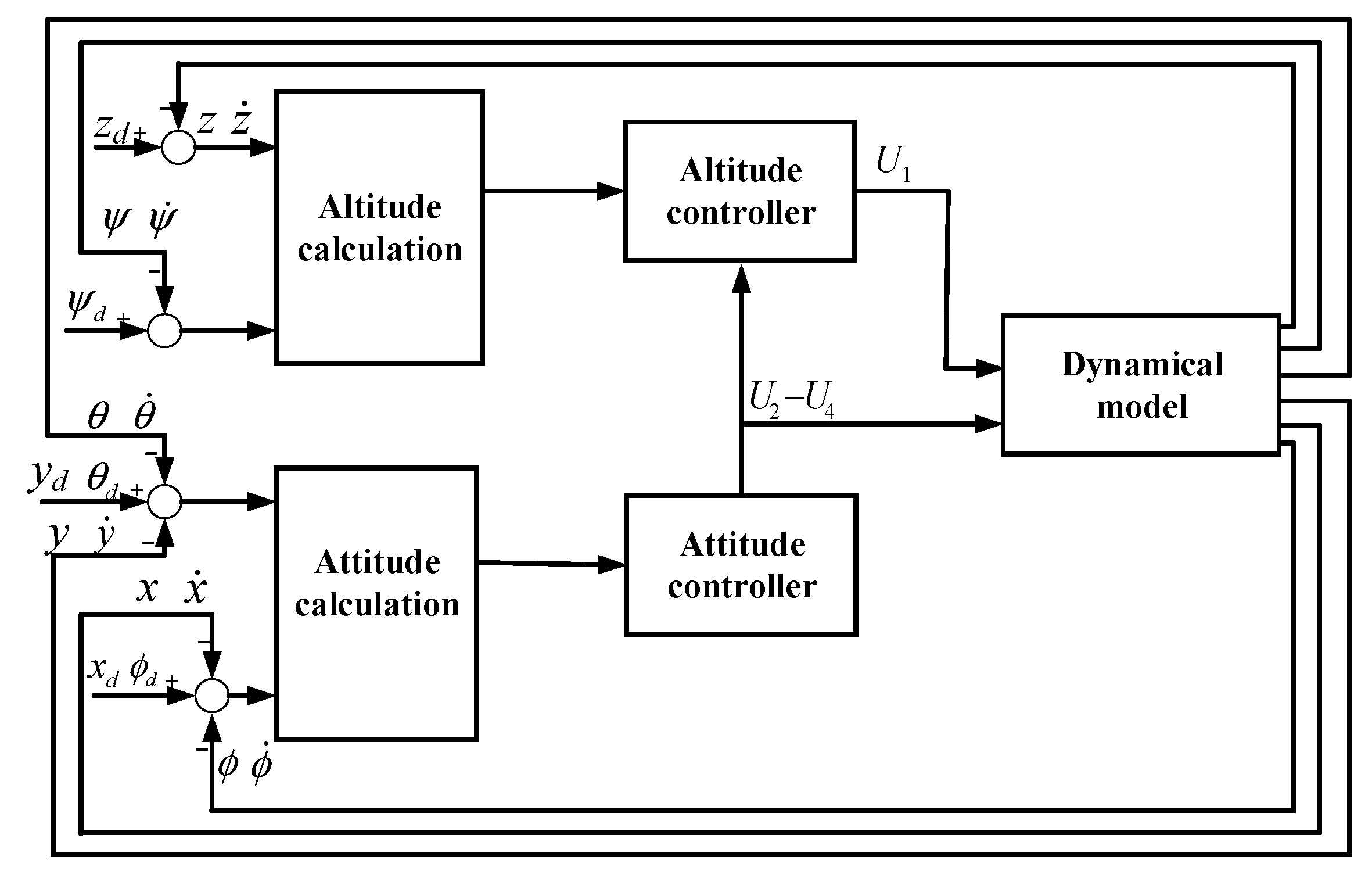
4. Controller Design
4.1. Overall Control Structure
4.2. Sliding Mode PID Control Algorithm
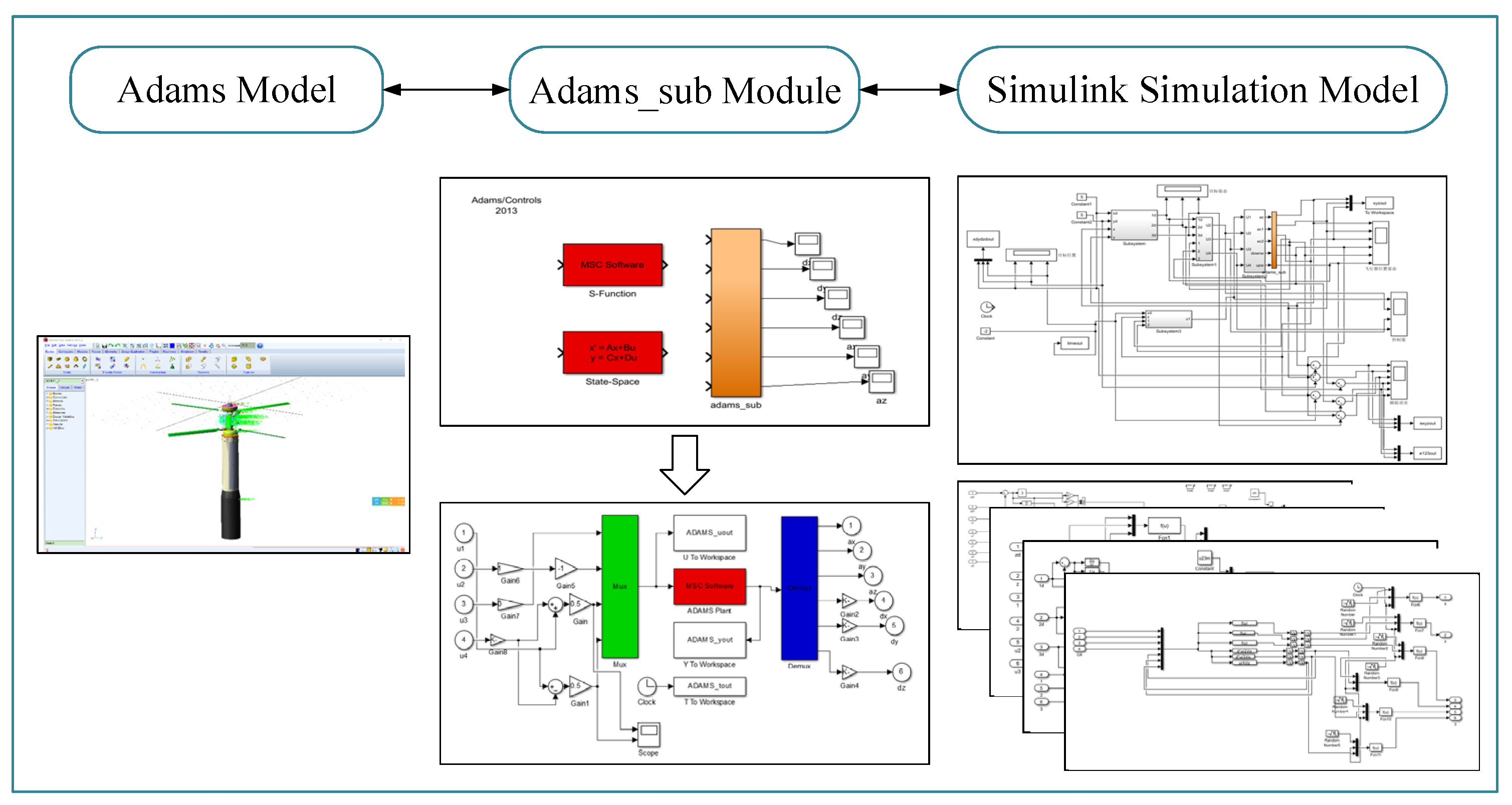
5. Joint Simulation of Adams/MATLAB
5.1. Simulation Model Establishment
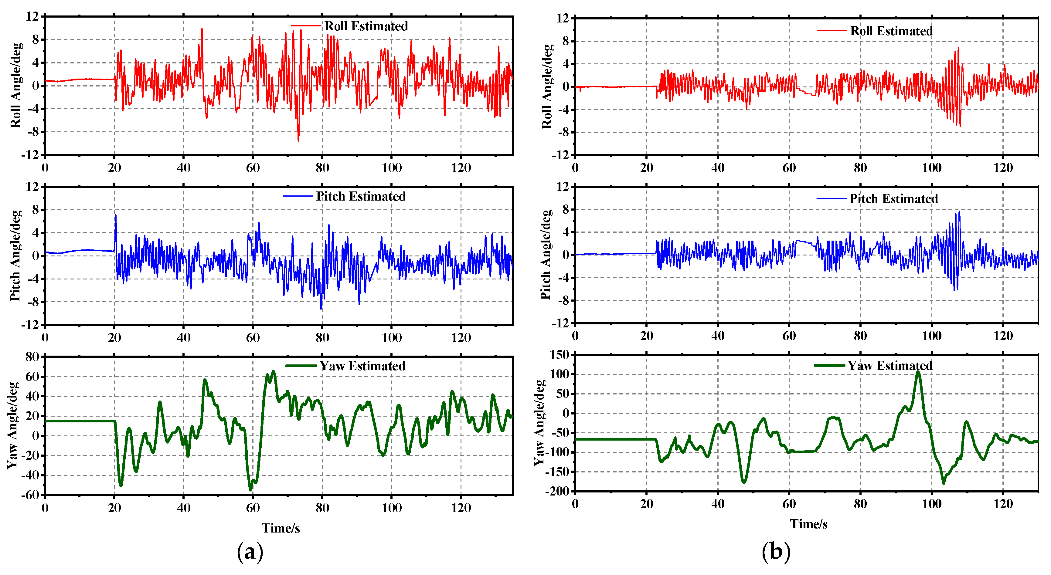
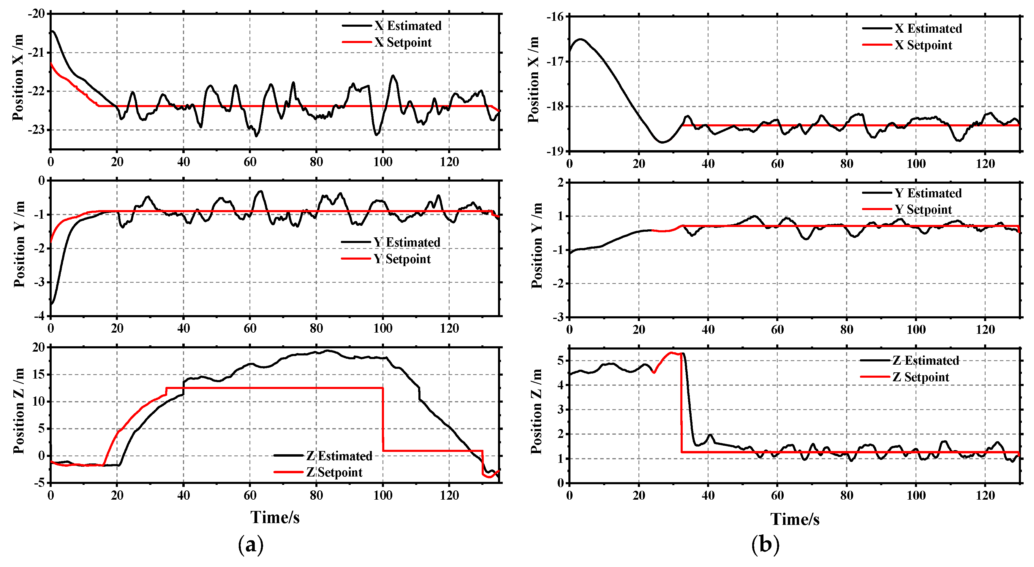
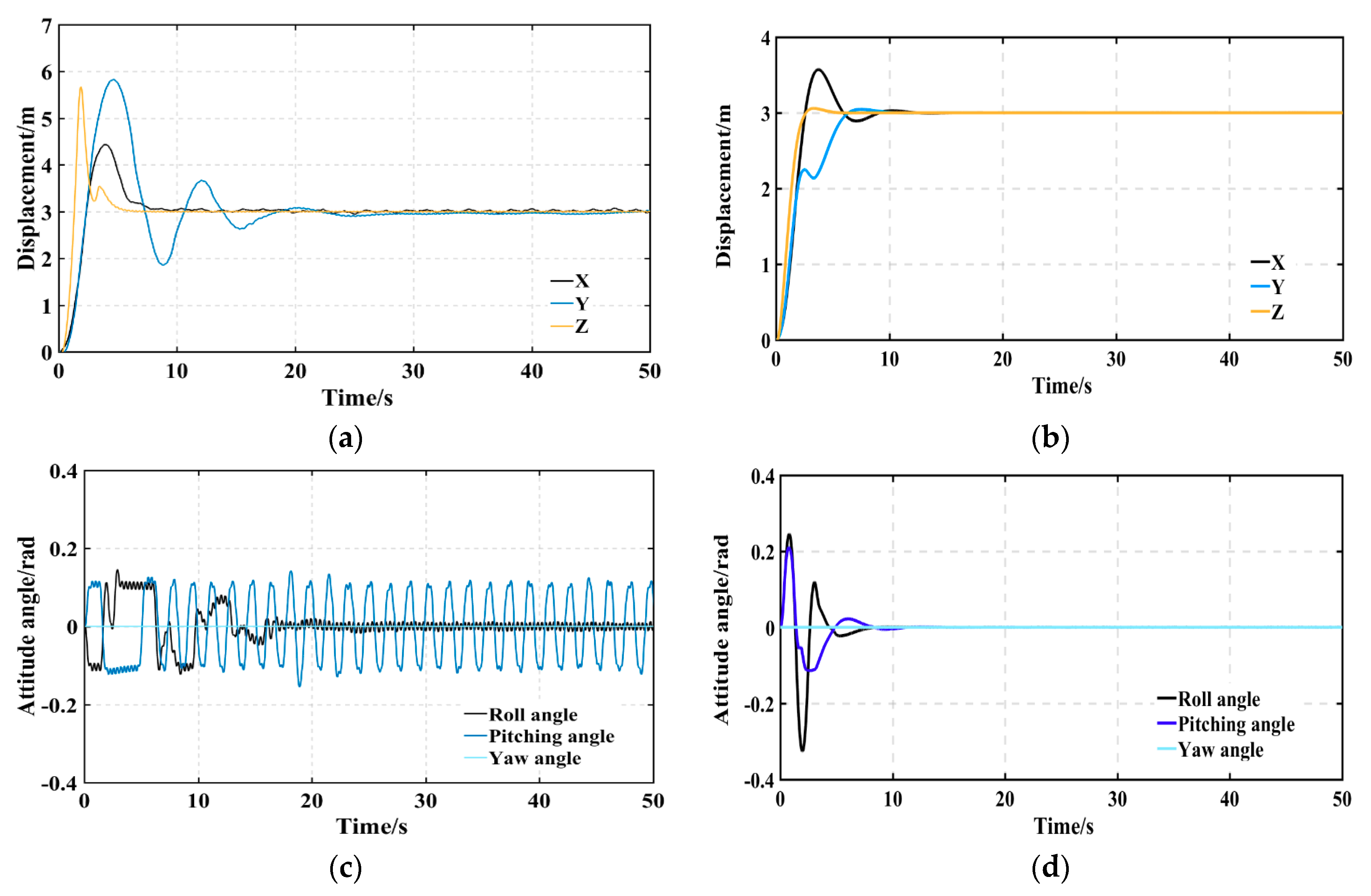
5.2. Hovering Simulation Results
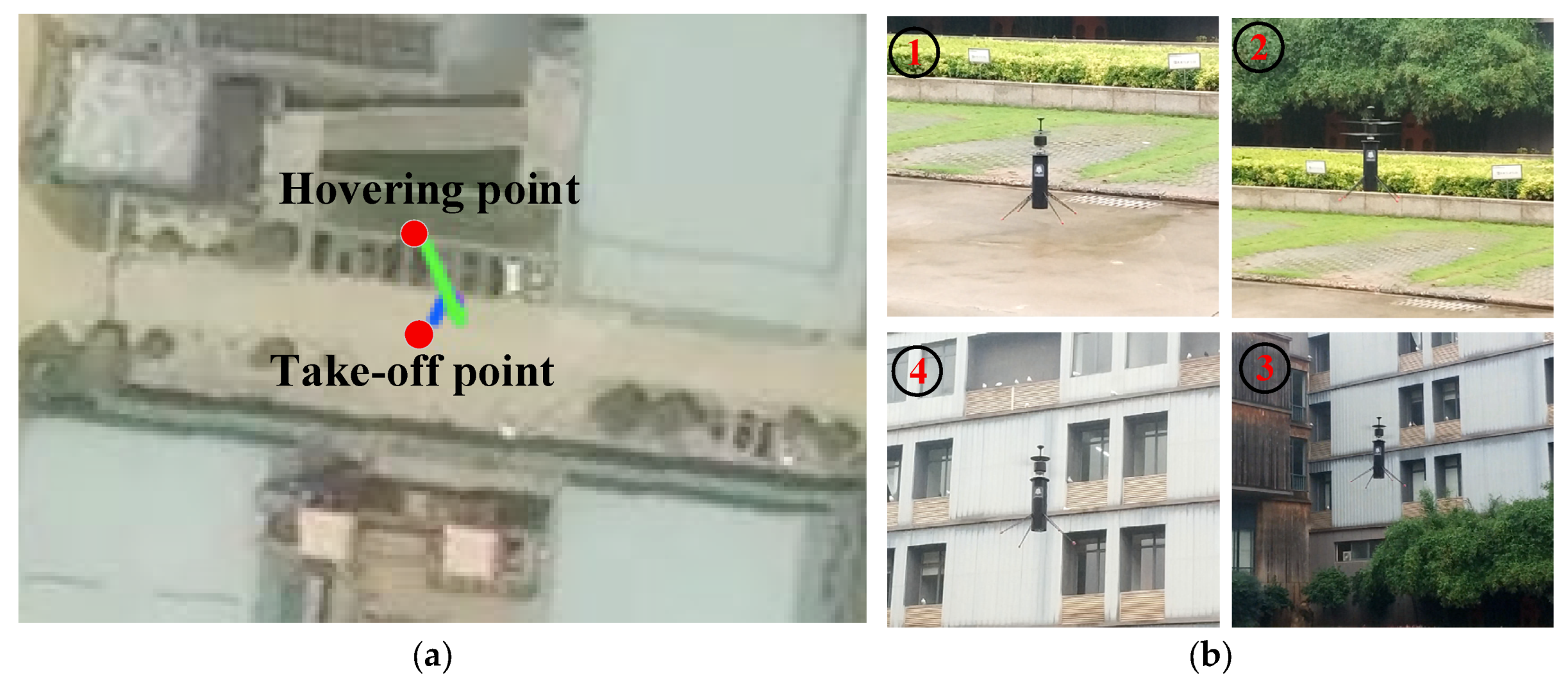
6. Experiments
7. Conclusions
Author Contributions
Funding
Acknowledgments
Conflicts of Interest
References
- Husnic, Z. Micro Coaxial Helicopter Controller Design. Ph.D. Thesis, Drexel University, Philadelphia, PA, USA, 2015. [Google Scholar]
- Chen, M. Technology Characteristic and Development of Coaxial rotor aircraft Helicopter. Aeronaut. Manuf. Technol. 2009, 17, 26–31. [Google Scholar]
- Mokhtari, M.R.; Cherki, B. Sliding mode control for a small coaxial rotorcraft UAV. In Proceedings of the 2015 3rd International Conference on Control, Engineering & Information Technology (CEIT), Tlemcen, Algeria, 25–27 May 2015; IEEE: Piscataway, NJ, USA, 2015. [Google Scholar]
- Mokhtari, M.R.; Cherki, B.; Braham, A.C. Disturbance observer based hierarchical control of coaxial-rotor UAV. ISA Trans. 2017, 67, 466–475. [Google Scholar] [CrossRef]
- Drouot, A.; Richard, E.; Boutayeb, M. Hierarchical backstepping-based control of a Gun Launched MAV in crosswinds: Theory and experiment. Control Eng. Pract. 2014, 25, 16–25. [Google Scholar] [CrossRef]
- Roussel, E.; Gnemmi, P.; Changey, S. Gun-Launched Micro Air Vehicle: Concept, challenges and results. In Proceedings of the 2013 International Conference on Unmanned Aircraft Systems (ICUAS), Atlanta, GA, USA, 28–31 May 2013; IEEE: Piscataway, NJ, USA, 2013. [Google Scholar]
- Gnemmi, P.; Changey, S.; Meder, K.; Roussel, E.; Rey, C.; Steinbach, C.; Berner, C. Conception and Manufacturing of a Projectile-Drone Hybrid System. IEEE/ASME Trans. Mechatron. 2017, 22, 940–951. [Google Scholar] [CrossRef]
- Lee, T.E. Design and Performance of a Ducted Coaxial rotor aircraft in Hover and Forward Flight. Ph.D. Thesis, University of Maryland, College Park, MD, USA, 2010. [Google Scholar]
- Giovanetti, E.B. Minimum Power Requirements and Optimal Rotor Design for Conventional, Compound, and Coaxial Helicopters Using Higher Harmonic Control. Ph.D. Thesis, Duke University, Durham, UK, 2013. [Google Scholar]
- Arama, B. Design and Implementation of a Hybrid Control Strategy for a Small Scale Coaxial rotor aircraft Helicopter. Ph.D. Thesis, Purdue University, West Lafayette, IN, USA, 2011. [Google Scholar]
- Espinoza, E.S.; Malo, A.; Lozano, R. Modeling and Sliding Mode Control of a Micro Helicopter-Airplane System. J. Intell. Robot. Syst. 2014, 73, 469–486. [Google Scholar] [CrossRef]
- Li, K.; Wei, Y.; Wang, C.; Deng, H. Longitudinal Attitude Control Decoupling Algorithm Based on the Fuzzy Sliding Mode of a Coaxial-Rotor UAV. Electronics 2019, 8, 107. [Google Scholar] [CrossRef]
- Bohorquez, F. Rotor Hover Performance and System Design of an Efficient Coaxial Rotary Wing Micro Air Vehicle. Ph.D. Thesis, Department of Aerospace Engineering, University of Maryland, College Park, MD, USA, 2007. [Google Scholar]
- Wicha, J. Coaxial rotor aircraft Hover Power Reduction Using Dissimilarity between Upper and Lower Rotor Design. Ph.D. Thesis, Rensselaer Polytechnic Institute, Troy, NY, USA, 2015. [Google Scholar]
- Xian, B.; Zhang, X.; Yang, S. Nonlinear controller design for an unmanned aerial vehicle with a slung-load. Control Theory Appl. 2016. [Google Scholar] [CrossRef]
- Wang, X.-L. C0-simuiating Study on the Vehicle’s Active Suspension Based on ADAMS and MATLAB. Ph.D. Thesis, Jilin University, Changchun, China, 2009. [Google Scholar]
- Yuan, X.; Zhu, J.; Chen, Z.; Lu, X. Kinematic modeling and analysis of a coaxial helicopter’s actuating mechanism. Acta Aeronaut. Astronaut. Sin. 2013, 34, 988–1000. [Google Scholar]
- Liu, Y.-P.; Huang, X.-J.; Li, X.-Y. Trajectory Tracking Control of Quad-rotor Unmanned Aerial Vehicles based on Sliding Mode PID. Mech. Sci. Technol. Aerosp. Eng. 2017, 36, 1859–1865. [Google Scholar]
- Johnson, W. Helicopter Theory. Airf. Eng. Aerosp. Technol. 2008, 12, 271–276. [Google Scholar]
- Dong, Z.-Y. Research on Modeling and Control Algorithm for Unmanned Coaxial rotor aircraft Helicopter. Ph.D. Thesis, Jilin University, Changchun, China, 2016. [Google Scholar]
- Chen, X.-Q. The Design & Research of the Flight Control System of Quadrotor. Ph.D. Thesis, Nanchang Hangkong University, Nanchang, China, 2014. [Google Scholar]
- Shi, Y.Q.; Li, M.Y.; Dun, X.M.; Liu, Q. Coordinated Simulation of Biped Robot Based on ADAMS and Matlab. Mach. Electron. 2008, 1, 45–47. [Google Scholar]


| Parameter | Value | Parameter | Value |
|---|---|---|---|
| 7.32 | 0.13 | ||
| 0.03 | 15.86 | ||
| 25 | 7.1 | ||
| 8.35 | 8.3 | ||
| 0.02 | 2.42 | ||
| 28 | 4 | ||
| 0.85 | 1 |
| Parameter | Value |
|---|---|
| Aircraft Mass m | 8.636 kg |
| Acceleration due to gravity g | 9.8 m/s2 |
| Distance from centroid to upper rotor L | 0.518 m |
| Rotor thrust coefficient CT | 0.0033 |
| Rotor solidity σ | 0.065 |
| blade section lift-curve slope a0 | 0.12 |
| Induced velocity | 7.98 m/s, 16.57 m/s |
| Rotor radius R | 0.385 m |
| Air density ρ | 1.29 kg/m3 |
| Aircraft roll moment of inertia Ix | 0.786 kg.m2 |
| Aircraft pitch moment of inertia Iy | 0.786 kg.m2 |
| Aircraft yaw moment of inertia Iz | 0.079 kg.m2 |
© 2019 by the authors. Licensee MDPI, Basel, Switzerland. This article is an open access article distributed under the terms and conditions of the Creative Commons Attribution (CC BY) license (http://creativecommons.org/licenses/by/4.0/).
Share and Cite
Wei, Y.; Chen, H.; Li, K.; Deng, H.; Li, D. Research on the Control Algorithm of Coaxial Rotor Aircraft based on Sliding Mode and PID. Electronics 2019, 8, 1428. https://doi.org/10.3390/electronics8121428
Wei Y, Chen H, Li K, Deng H, Li D. Research on the Control Algorithm of Coaxial Rotor Aircraft based on Sliding Mode and PID. Electronics. 2019; 8(12):1428. https://doi.org/10.3390/electronics8121428
Chicago/Turabian StyleWei, Yiran, Han Chen, Kewei Li, Hongbin Deng, and Dongfang Li. 2019. "Research on the Control Algorithm of Coaxial Rotor Aircraft based on Sliding Mode and PID" Electronics 8, no. 12: 1428. https://doi.org/10.3390/electronics8121428
APA StyleWei, Y., Chen, H., Li, K., Deng, H., & Li, D. (2019). Research on the Control Algorithm of Coaxial Rotor Aircraft based on Sliding Mode and PID. Electronics, 8(12), 1428. https://doi.org/10.3390/electronics8121428