Article

Efficient Evolutionary Learning Algorithm for Real-Time Embedded Vision Applications

1
School of Electrical and Computer Engineering, Nanfang College of Sun Yat-sen University, Guangzhou 510970, China
2
Department of Electrical and Computer Engineering, Brigham Young University, Provo, UT 84602, USA
*
Author to whom correspondence should be addressed.
Electronics 2019, 8(11), 1367; https://doi.org/10.3390/electronics8111367
Submission received: 26 October 2019 / Revised: 13 November 2019 / Accepted: 16 November 2019 / Published: 18 November 2019
(This article belongs to the Section Computer Science & Engineering)

Abstract

:
This paper reports the development of an efficient evolutionary learning algorithm designed specifically for real-time embedded visual inspection applications. The proposed evolutionary learning algorithm constructs image features as a series of image transforms for image classification and is suitable for resource-limited systems. This algorithm requires only a small number of images and time for training. It does not depend on handcrafted features or manual tuning of parameters and is generalized to be versatile for visual inspection applications. This allows the system to be configured on the fly for different applications and by an operator without extensive experience. An embedded vision system, equipped with an ARM processor running Linux, is capable of performing at roughly one hundred 640 × 480 frames per second which is more than adequate for real-time visual inspection applications. As example applications, three image datasets were created to test the performance of this algorithm. The first dataset was used to demonstrate the suitability of the algorithm for visual inspection automation applications. This experiment combined two applications to make it a more challenging test. One application was for separating fertilized and unfertilized eggs. The other one was for detecting two common defects on the eggshell. Two other datasets were created for road condition classification and pavement quality evaluation. The proposed algorithm was 100% for fertilized egg detection and 98.6% for eggshell quality inspection for a combined 99.1% accuracy. It had an accuracy of 92% for the road condition classification and 100% for pavement quality evaluation.

1. Introduction

Process automation is a current trend and the main focus of many industries to improve their competitiveness. Labor shortages, increasing labor costs, and the demand for high-quality products are the forces driving this movement. Locating and hiring experienced workers has become a challenging administrative task worldwide. Of the many areas in manufacturing that require an upgrade to cope with these challenges, visual inspection cannot be ignored. It is used to prevent defective or low-quality products from reaching the market and to detect and correct problematic processes in the early processing stages to reduce waste. Visual inspection is a labor-intensive process and constitutes a sizable portion of production expense. These challenges have become even more prevalent in recent years.
There are many off-the-shelf vision systems that are designed to perform vision tasks at an affordable price. These systems have simple built-in software tools that are designed to allow an experienced end user to install, configure, and operate them. Most of these tools use common image processing techniques or depend on a human expert to design the relevant features to perform the desired object recognition or visual inspection tasks. Although the hand-crafted features are able to describe the object of interest well and produce sound accuracy, specific features created by human experts that are good for one class of products may do poorly for others. This manual process often involves the redesigning of the algorithms or fine-tuning of inspection parameters that requires unique skills and extensive training. Even if possible, these added challenges make these off-the-shelf systems unsuitable for many vision applications that require sophisticated image classification and visual inspection capabilities.
The key to building a visual inspection system is to construct distinctive features or representations of data from high-dimensional observations such as images and videos. A good set of relevant visual features must be constructed in order to have a good representation of the input data. Methods, such as feature selection, feature extraction, and feature construction, have been used to obtain high-quality features [1,2,3]. Feature selection is the process of selecting a subset of distinctive features from a large set of features [1]. A subset of features can be generated by gradually adding selective features into an empty set or removing the less effective features from the original feature space according to some predetermined criteria. Feature extraction is the process of extracting a set of new features from the original features by applying functional mappings. Feature construction is the process of discovering discriminative information or subtle differences among images. All three types of approaches are developed to improve feature quality and achieve accurate image classification.
Many feature learning approaches using evolutionary techniques have been proposed over the past few years. A comprehensive survey of the state-of-the-art work on evolutionary computation for feature selection is presented in Reference [4]. Krawiec and Bhanu [5] used a genetic algorithm to obtain a fixed-length feature vector that is defined as a sequence of image processing operations and feature extraction steps. Wang et al. [6] used particle swarm optimization to perform feature selection and show that particle swarm optimization is effective for rough set-based feature selection. Sun et al. used a genetic algorithm to select a subset of eigenvectors rather than the traditional method of simply taking the top eigenvectors. Their method was tested for vehicle and face detection [7]. Sherrah et al. also used a genetic algorithm to determine whether a feature pre-processing step is necessary before classification [8]. Genetic algorithm has also been used to automatically optimize the selection of the optimal features for classification or remote sensing data [9]. This method aims to reduce the feature dimensionality by exploiting the genetic algorithm. Sian and Alfred proposed an evolutionary-based feature construction approach for relational data summarization [10]. This method addresses the problem of many-to-one relationships that exist between non-target tables and target tables and improves the accuracy of the summarized data.
None of the aforementioned feature learning approaches aims at constructing or selecting features for general image classification. They mostly perform well on a single dataset for a specific application. We believe that a good feature learning algorithm should be able to automatically generate sufficient high-quality and unique features to perform accurate image classification.
Genetic algorithms [11], as one of the most popular evolutionary computation techniques, are inspired by the process of natural selection. A population of candidate solutions to a specific optimization problem is evolved toward better solutions in genetic algorithms. Each candidate solution has a set of properties which can be altered during the evolution process.
Evolutionary learning techniques are a good choice for image classification. Genetic algorithm (GA) is an evolutionary computation technique that automatically evolves solutions based on the idea of the survival of the fittest. It is a very flexible heuristic technique that allows us to use various types of feature representations in the learning process. The application of genetic algorithm to object recognition offers many advantages. The main one is its flexibility which enables the technique to be adapted for each particular problem [12]. The flexibility of GA in representing and evolving a wide range of models makes it a very powerful and convenient method with regard to classification.
Tran et al. used a GA with a multi-tree representation method to construct a much smaller number of new features than the original set on high-dimensional datasets in classification [13]. A comprehensive survey on the application of GA to classification is given in Reference [12]. Genetic algorithms have been successfully applied to feature construction methods [14,15]. In those methods, richer features can be constructed by applying operators to primitive features. Genetic algorithms are also used to construct multiple high-level features by adopting an embedded approach and the result shows that those high-level features constructed by the GA are effective in improving the classification performance, in most cases, over the original set of features [16].
In this work, we aimed at developing an efficient evolutionary learning algorithm for embedded visual inspection and mobile computing applications. Compared with more general object recognition tasks, visual inspection applications often have a small number of classes and are inconvenient, if possible, to obtain a large number of images for training. Our goal was to find an efficient algorithm that can achieve an acceptable balance between the accuracy and simplicity of the system for embedded visual inspection applications.
This work built upon our previous success in using a genetic algorithm for feature construction tasks for object recognition and classification [17,18]. As a data-driven approach, the ECO-Feature algorithm automatically discovers salient features from a training dataset without the involvement of a human expert. It is a fully automated feature construction method. Experimental results confirmed that it is capable of constructing non-intuitive features that are often overlooked by human experts. This unique capability allows easy adaption of this technology for various object classes when the differentiation among them is not defined or cannot be well described.
We improved our algorithm since its first introduction by constructing global features from the whole image to make it more robust to image distortions than the original version that used local features [19]. We then reduced the feature dimensionality to speed up the training process [20]. Constructing global features proven to increase classification performance [19]. The main weakness of the ECO-Feature algorithm is that it is designed only for binary classification that cannot be directly applied to multi-class cases. We also observe that the recognition performance depends heavily on the size of the features pool from which features can be selected and the ability of selecting the best features. This makes it difficult to determine how many features need to be constructed from the images in order to achieve the best performance.
An enhanced evolutionary learning method for multi-class image classification was developed to address the aforementioned challenges. Among other improvements, boosting was added to select the features and combine them into a strong classifier for multi-class classification. These characteristics allow the proposed algorithm to require fewer features for classification and, hence, make it more efficient. There is no doubt that other classification methods can perform as well as the proposed evolutionary learning algorithm but most of them either require handcrafted features or computational power. We included three experiments in this paper to demonstrate the performance of the proposed algorithm.
Most egg farms use manual labor to grade and inspect eggs. Human visual inspection only detects broken eggs during the process. Very few egg farms use machines to measure the size of an egg, detect defects, or to separate fertilized eggs to improve hatching efficiency. To increase revenue and ensure product quality, an automated grading and inspection machine is needed. We created one dataset for the combined experiment of two applications. It included images of fertilized and unfertilized (normal) eggs for unfertilized egg detection and removal application for the chicken hatching process. It also included images of normal eggs and eggs with dirt or cracks on the shell for egg quality evaluation applications for egg production. These were two completely different applications. We combined them to make it a challenging experiment for testing the robustness of the proposed evolutional learning algorithm.
Just as a human driver changes his or her defense mechanisms against road surface conditions, a self-driving car or an advanced driver assistance system (ADAS) must do the same. Without the input of the road condition, the system will not be able to adapt its control of the vehicle for different road conditions. Using standard autonomous driving actions for all road conditions increases the risk for accidents. Automatic evaluation of road surface condition is considered an important part of an autonomous vehicle driving system [21]. We created two datasets for this experiment. One dataset included images of dry, wet, and sandy roads as well as roads covered with snow, ice, and a puddle of water for road condition detection. The other dataset included images of pavement with different levels of damage for pavement quality evaluation.

2. Algorithm

Although quite successful, our original ECO-Feature algorithm was designed only for binary classification that cannot be directly applied to multi-class cases [17,18]. We also observe that the recognition performance depends heavily on the size of the features pool from which features can be selected and the ability of selecting the best features. This makes it difficult to determine how many features need to be constructed from the images in order to achieve the best performance. We developed an enhanced evolutionary learning method for multi-class image classification to address the aforementioned challenges and applied it to four applications.
Our evolutionary learning algorithm uses evolutionary computation to construct a series of image transforms that convert the input raw pixels into high-quality image representations or features. This unique method extracts features that are often overlooked by humans and is robust to minor image distortion and geometric transformations. It uses boosting techniques to automatically construct features from training data without the use of a human expert. It is developed for multi-class image classification.
In this work, we aimed to develop an efficient image classification algorithm using evolutionary strategies for multi-class visual inspection applications for embedded vision systems. We recognize that there are many other more sophisticated and powerful methods such as machine learning and new and popular deep learning approaches that could be more capable than the proposed evolutionary learning algorithm [22,23]. Most of them are often overkill for our applications and require expensive computational power, a large number of images for training, long training time, and slow classification. Because of their complexity, they can hardly be considered friendly for hardware implementation. All these requirements are viewed as constraints to providing a low-cost embedded vision system for automatic visual inspection which is the main objective of this research. Our algorithm is able to run at close to 100 frames per second with an ARM processor running Linux.

2.1. Evolutionary Learning

In our algorithm, phenotypes in the genetic algorithm represent our evolutionary image transformations or the often-called image features. The genes which make up a phenotype consist of a number of select basic image transforms and their corresponding parameters. The number of genes that can be modified for each evolutionary transformation varies, since both the number of transforms and the number of parameters for each transform vary.
Each phenotype in the population represents a possible evolutionary image transformation. A fitness score is computed for each phenotype using a fitness function. A portion of the population is then selected to create a new generation. We used a tournament selection method to select phenotypes from the overall population in the genetic algorithm. In order to produce a new transformation, a pair of parent phenotypes is selected to undergo certain evolution operations including crossover and mutation.
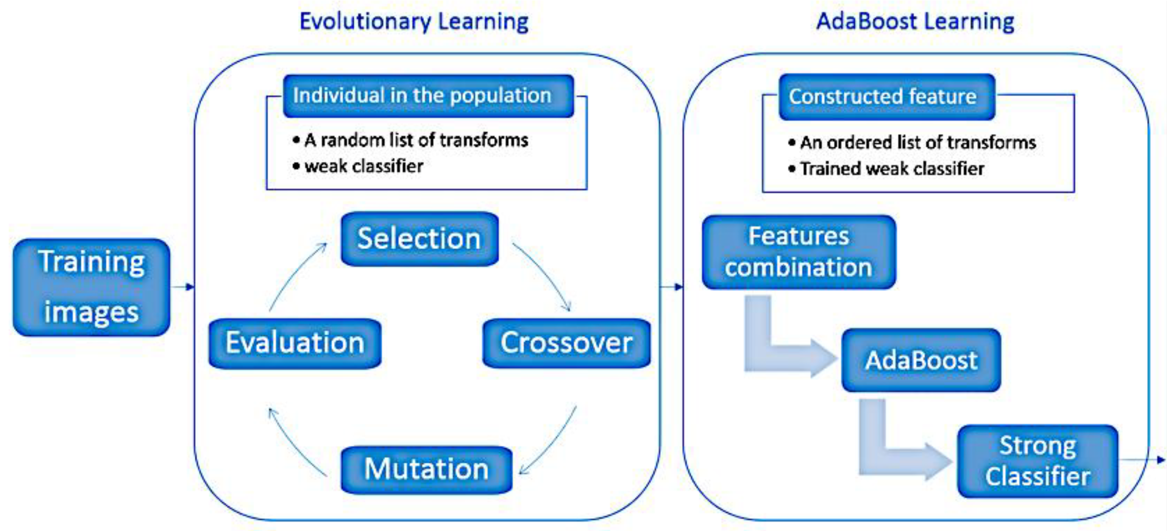
The crossover in our method is done by rearranging the image transforms from both parents. By using crossover and mutation, a new phenotype, typically sharing many characteristics of its parents, is created. This process results in the next generation of image transformations that are different from their parent generation. Hence, the new phenotypes are likely to have a different number of image transforms and parameters. This process is repeated for several generations, evolving image features with high fitness. The evolution is terminated when a satisfactory fitness score is reached or the best fitness score remains stable for several iterations. Figure 1 shows an overview of the training process of the proposed algorithm.

2.2. Evolutionary Image Transformation

The representation of a phenotype in our genetic algorithm is an important factor influencing the performance of the algorithm. An evolutionary image transformation or an image feature is constructed using a series of image transforms that is created by the genetic algorithm. Rather than applying a single image transform to the image, we constructed the transformation by applying a sequence of basic image transforms to the input image. This process is defined in Equation (1), where V is the evolutionary image transformation output vector, n is the number of transforms an evolutionary image transformation is composed of, I defines an input image, Ti represents each transform at step i, and ϕ i is the corresponding parameter vector of each transform at step i.
V 1 =   T 1 ( I ,   ϕ 1 ) V n     1 =   T n 1 ( V n     2 , ϕ n     1 ) V   =   T n ( V n     1 , ϕ n )
Based on this definition of the evolutionary image transformation, the output of one transform is the input to the next transform. An evolutionary image transformation is learned through the evolution of this sequence of transforms. All transforms included in our algorithm are basic image transforms that can be found in almost all open source computer vision libraries. Twenty-four transforms were included in our original version [17,18]. In this improved version, we focused on efficiency and included only those that are filter-based and hardware friendly. Six transforms chosen for our genetic algorithm were Gabor (two wavelengths and four orientations), Gaussian (kernel size), Laplacian (kernel size), Median Blur (kernel size), Sobel (depth, kernel size, x order, y order), and Gradient (kernel size), with the parameters in parentheses. We chose these six simple transforms for their simplicity and noise removal, edge detection, and texture and shape analysis characteristics. They were not chosen for any specific applications. This set of transforms can be extended to include almost any image transforms, but we are mostly interested in those transforms that are able to extract important information from images and are simple and efficient. Using these image transforms in our method provides the system with the basic tools for feature extraction and helps speed up the evolutionary learning process.
For each transformation sequence during the evolution, its length or the number of transforms that make up the transformation sequence is not fixed. Rather, it is randomly selected by the genetic algorithm. During training, for example, our algorithm tries out different sizes of kernel for the Gaussian (variance is dependent on the kernel size), Median (blurring level is dependent on the kernel size), Laplacian (blurring and sharpening level is dependent on the kernel size), and Gradient (gradient is dependent on the kernel size) filters and automatically selects their sizes to be the most discriminant for classification. The other two transforms (Gabor and Sobel) have 6 and 4 parameters to be tried and selected by the algorithm also automatically. The type and order of the transforms in a transformation sequence and their parameters are determined by the evolution process. As a result, it is possible that any one transform from our list can be used more than once in a sequence but with different parameters.
The number of transforms, n in Equation (1), used to create an initial evolutionary transformation varies from 2 to 8 transforms. The range of 2 to 8 transforms allows the algorithm to yield good result while keeping the computation efficient and simple.

2.3. Fitness Score Calculation

As described above, a candidate image transformation or feature is constructed using a sequence of selected image transforms with their selected parameter values. Its performance must be evaluated to determine if it is indeed a good and discriminative feature for classification. A fitness function, which is designed specifically for classification, is used to compute a fitness score to evaluate how good the image transformation is during the evolution process.
We calculated a fitness score for each evolutionary image transformation based on its classification performance using a simple classifier. The classifier is trained for each image transformation using the training images and the classification performance is computed with the validation images. The fitness score is an indication of how well this classifier performs on the images.
The fitness score for each evolutionary image transformation is computed using Equation (2). It is defined based on the classification accuracy of the classifier that is associated with each constructed evolutionary image transformation. It reflects how well the classifier classifies images. Classification accuracy is a fairly generic measure for optimization; quality measures other than accuracy can be used depending on the application.
f i t n e s s =   100 × # c o r r e c t l y   c l a s s i f i e d # t o t a l   i m a g e s
Due to the fact that the evolution requires iterating over several generations to produce satisfactory results, this classification-based fitness function must be efficiently computable. It also should be a multi-class classifier that can be easily applied to many multi-class image classification cases. Random forest classifier was chosen as the classifier to evaluate the performance of each image transformation in our method. Random forest classifier is ranked as one of the top classifiers among the 179 classifiers that have been evaluated in extensive experiments [24]. The authors claim that the best results are achieved by the random forest classifier. Random forest shows the advantage of high computational efficiency over other popular classifiers such as SVM [25]. Random forest is regarded as a multi-class classifier that is robust against noise, has high discrimination performance, and is capable of training and classifying at high speed [26].
Random forest is an ensemble learning algorithm that constructs multiple decision trees. It works by randomly selecting training samples for tree construction, resulting in the construction of a classifier that is robust against noise. Random forest classifier has shown to be efficient with good generalization performance due to the fact of its randomness in training [25]. Also, the random selection of features to be used at each node enables fast training, even when the dimensionality of the feature vector is high [24].

2.4. Selection and Combination of Learned Features

Genetic algorithm simulates the survival of the fittest among individuals over generations and one best evolutionary image transformation is obtained at the end of each simulated evolution run. Though one single evolutionary image transformation usually has a high discrimination ability in image classification, using multiple transformations can often increase performance. It is difficult to determine how many learned transformations are needed for a specific application, and due to the randomness of our method, it may require a large pool of learned transformations in order to maintain stable performance. For this reason, boosting is employed in our framework to maintain high classification performance even with a small number of learned image transformations due to the fact that sequential training in boosting constructs complementary classifiers from the training examples.
AdaBoost is one variant of a popular boosting algorithm proposed by Freund and Schapire [27] and is used to combine a number of weak classifiers to make a stronger classifier. Various multi-class boosting algorithms such as AdaBoost.M1 and AdaBoost.MH were proposed [28,29]. They both deal with multi-class classification problems with combinations of binary classification. Reference [30] proposed a novel multi-class boosting algorithm which is referred to as Stagewise Additive Modeling using a Multi-class Exponential loss function (SAMME). The SAMME algorithm directly extends the AdaBoost algorithm to multi-class classification rather than reducing it to two-class classifications. It is the natural extension of the AdaBoost algorithm to the multi-class case, and its performance is comparable with that of AdaBoost.MH and sometimes slightly better [30].
The training process of the SAMME classifier in our method involves reweighting the training examples within each iteration right after an evolutionary image feature is learned from the raw pixel images. The SAMME iteratively builds an ensemble of multi-class classifiers and adjusts the weights of each training example based on the performance of the weak classifier that is associated with the learned image feature in the current iteration. Examples that are misclassified will have their weights increased, while those that are correctly classified will have their weights decreased. Therefore, in subsequent iterations, the resulting classifiers are more likely to correctly classify examples that are misclassified in the current iteration.
In particular, given a training dataset {( x 1 ,   y 1 ) ,   , ( x m ,   y m ) }, where x i X is the input signal and y i Y = { 1 ,   2 ,   ,   K } is the corresponding class label, SAMME sequentially trains M weak classifiers with the training dataset and calculates a weight α m for the mth classifier T m based on the following equation:
α m = log 1 error m error m + log ( K 1 ) ,
where e r r o r m is the error calculated for the weak classifier T m .
The SAMME algorithm is very similar to AdaBoost but with a major difference in Equation (3). In order for α m to be positive for each weak classifier, we only need the accuracy of each weak classifier to be better than the random guessing accuracy rate 1/K which depends on the number of classes. When comparing the SAMME algorithm with the AdaBoost algorithm, AdaBoost breaks after the error goes above 50%. Thus, in AdaBoost, it is required that the error of each weak classifier be less than 50%, and this requirement is much harder to achieve than 1/K in SAMME. However, for the SAMME algorithm, because of the extra term log ( K 1 ) in Equation (3), α m can still be positive even though the error of each weak classifier goes over 50%.
After training, the resulting SAMME model consists of a list of weak classifiers and coefficients α m that indicate how much to trust each weak classifier in the model. The output of all weak classifiers is combined into a weighted sum that represents the final output of the boosted classifier:
C ( x ) = arg max k m :   T m ( x )   =   k M α m
where M is the number of weak classifiers in the SAMME model, T m is the mth weak classifier, α m is the weight for classifier T m , and k is the classification label for each class.

3. Experiments

We created three datasets for visual inspection and mobile visual computing applications. The first dataset included images of fertilized and unfertilized eggs for detecting and removing unfertilized eggs and images of good eggs and eggs with two common defects (crack and dirt) that are to be detected and removed during egg production process. Detecting and removing unfertilized eggs is important for chicken hatcheries as a means to cut production costs. Egg defect detection is important for egg production to ensure high product quality. We combined these two applications to perform a more challenging test with four classes. The second dataset included images of dry, wet, and sandy roads as well as roads covered with snow, ice, and puddles of water for road surface condition detection. The last dataset included images of pavement with different levels of damage for pavement quality evaluation.
We performed the training multiple times for all three experiments on a desktop computer using our training images for 80 iterations to obtain between 30 to 50 features. We then ran the classification using the learned features on an embedded system equipped with a Cortex-A15 2 GHz processor. The processing time was approximately 10 milliseconds per prediction or 100 frames per second. Our algorithm proved to be efficient for very high frame rate performance even with a small ARM-based processor.
We recognize that these three sample applications might be viewed as straightforward cases and many other approaches could work just as well as the proposed method. As emphasized previously, our aim was to develop an efficient (fast and requiring very few training images) and easy-to-configure method that is versatile and does not depend on handcrafted features or manual tuning of parameters. These three applications clearly demonstrate the versatility of the proposed evolutionary learning algorithm.

3.1. Egg Quality Evaluation

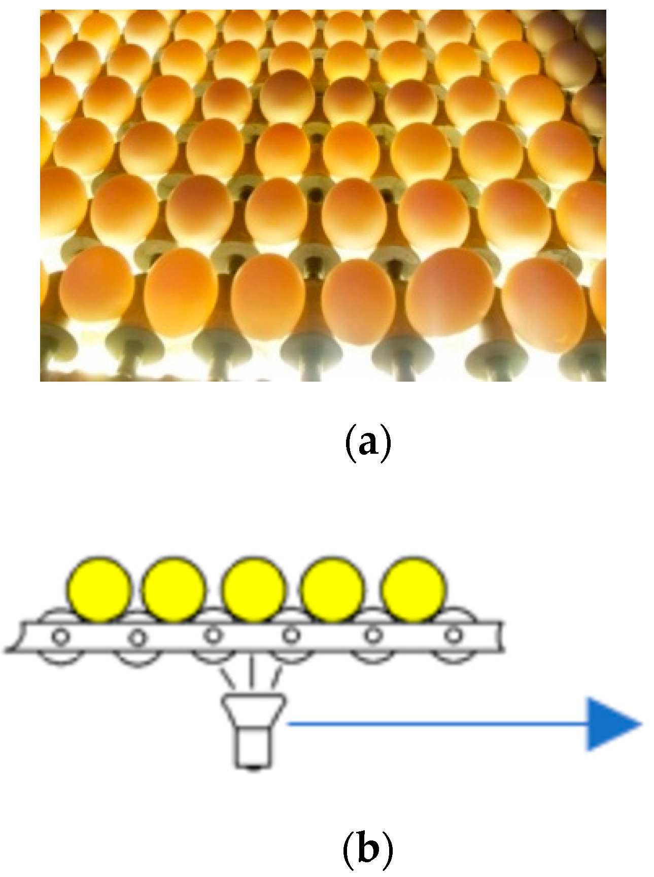
Figure 2a shows a photo taken from an egg processing plant. It shows a candling station where a worker uses a handheld sensor to point to and register the defective eggs in the system which then directs the machine to remove them. As shown in Figure 2a, the best and most common lighting for manual visual inspection is backlight, often referred to as candling. Figure 2b illustrates the egg candling setup. This manual candling is slow and often unreliable. In our study, all collected samples are imaged with backlight.
Samples of egg images captured with backlight are shown in Figure 3. From left to right, they are a good egg, egg with cracks and dirt, and a fertilized egg. The size of the egg is graded by weight using the load cells on the machine and is not discussed here. The samples used in this study were all white-shelled eggs of which 500 were good eggs, 139 had cracks, 233 had dirt on the shell, and 498 were fertilized eggs (hatched between 5 to 9 days). We used 75% of these samples for training and 25% for testing.

3.1.1. Performance

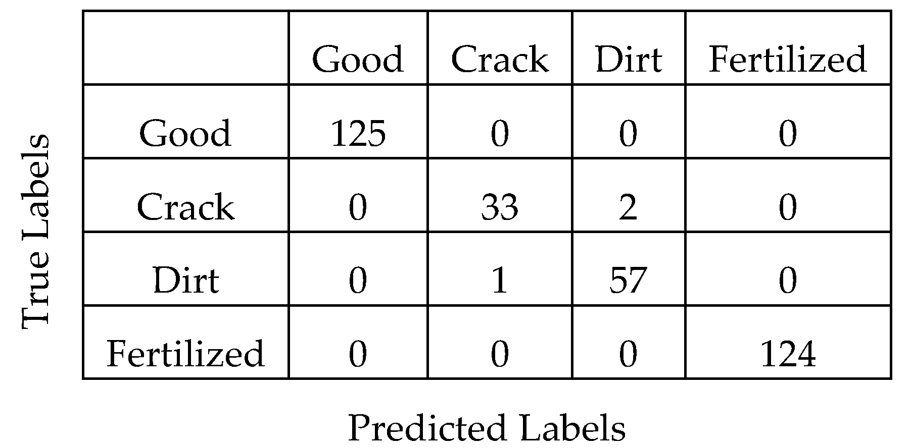
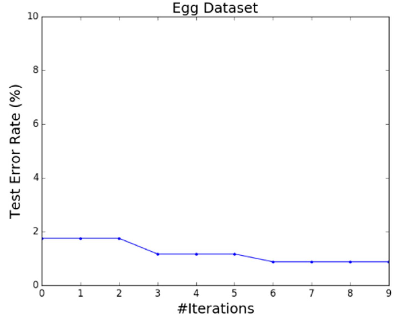
The proposed evolutionary learning algorithm obtained a 99.1% classification accuracy on our egg dataset. Figure 4 shows the confusion matrix for this experiment. All good and fertilized eggs were correctly classified. Two eggs with cracks were misclassified as dirt and one egg with dirt was misclassified as crack. All other test images were classified correctly. The classification performance of each iteration in the evolutionary learning on this dataset is shown in Figure 5. It took our evolutionary learning algorithm only six learning iterations or evolutionary generations to reach its steady-state performance.

3.1.2. Features from Evolutionary Learning

Our evolutionary learning method is generalized that it can be easily applied to different applications without a human expert to adjust any parameters or design specific image features. We took a closer look at what those image features obtained from the learning process were composed of and the proposed evolutionary learning algorithm constructed for this application.
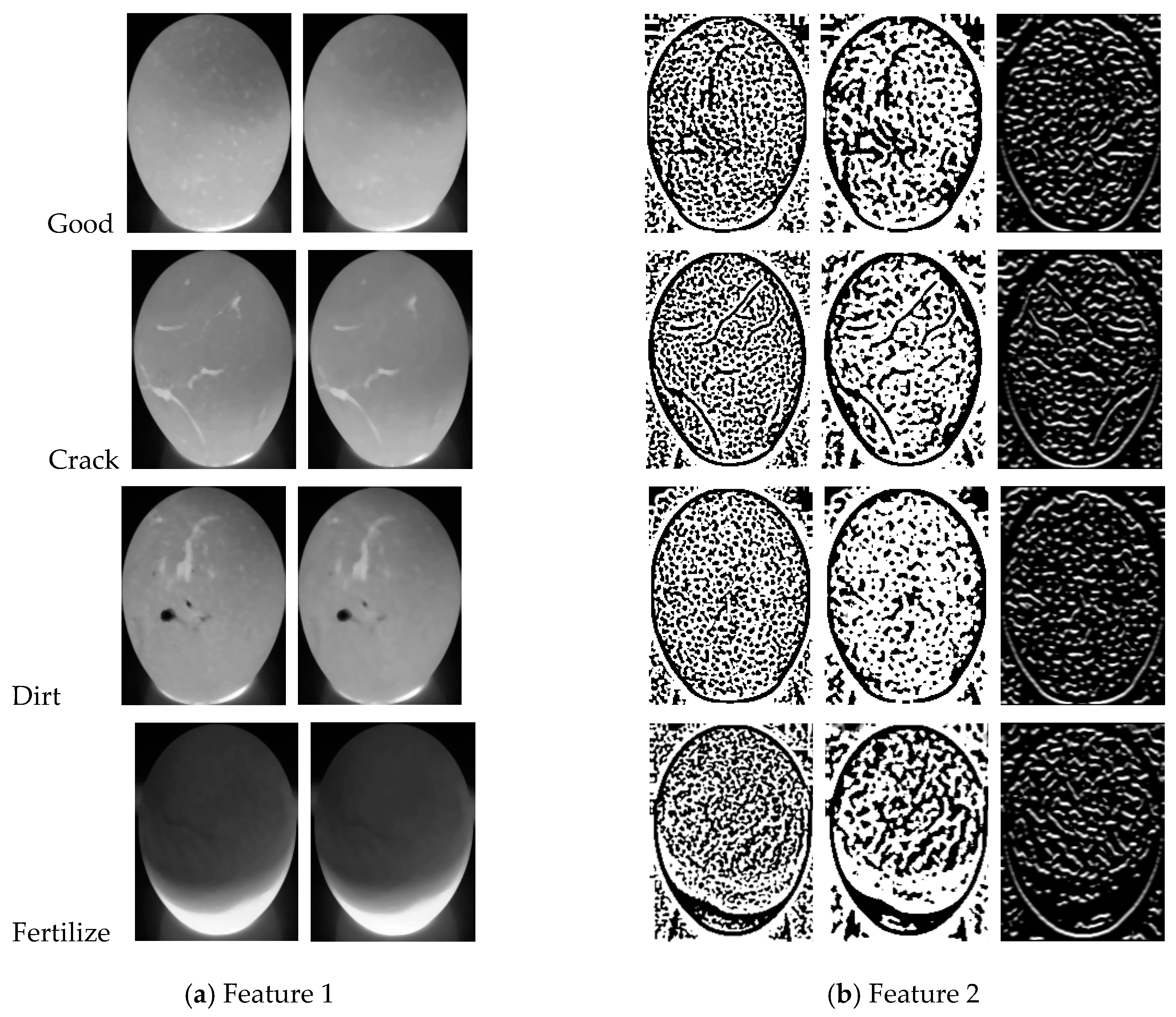
Our method constructed a group of evolutionary image transformations or features that are composed of a series of image transforms. The information these transformations discovered can be analyzed by examining the output of each image transform in the learned transform sequences. The image transform output of each training image is different, because every training image in the same class is slightly different. We selected one image transform output of the training images used for each specific class to visualize the feature.
Figure 6 shows two of ten features (genes) learned from the egg dataset used in this paper. Each row represents a class of the egg and each column represents a particular transform that is used in that feature. These transforms (from left to right) are shown in the order they appear in the feature. To be more specific, the first feature (Figure 6a) had 2 median blur transforms, both with a kernel size of five. The second feature (Figure 6b) had three transforms. This feature consisted of a Laplacian transform with a kernel size of nine, a median blur transform with a kernel size of five, and a Sobel operator with kernel size of seven. These are only two of the thirty features that were learned from the evolutionary learning. They may not seem significant or distinctive but are sufficient for our simple task.

3.2. Road Condition Detection

We evaluated our evolutionary algorithm on another two datasets that were created for this work. These two datasets consisted of images obtained from the Internet and recorded videos in real-world conditions. We implemented our multi-class boosting algorithms using resampling rather than reweighting because it performs just as well or significantly better in some cases [31]. In our boosting model, we used sampling with replacement to reflect example weights. A new training dataset with the same size as the original training dataset was assembled by sampling from the original training dataset, where the probability that any example to be selected is proportional to its assigned weight. The image feature learned from this resampled training data therefore places more emphasis on those examples with higher weights.
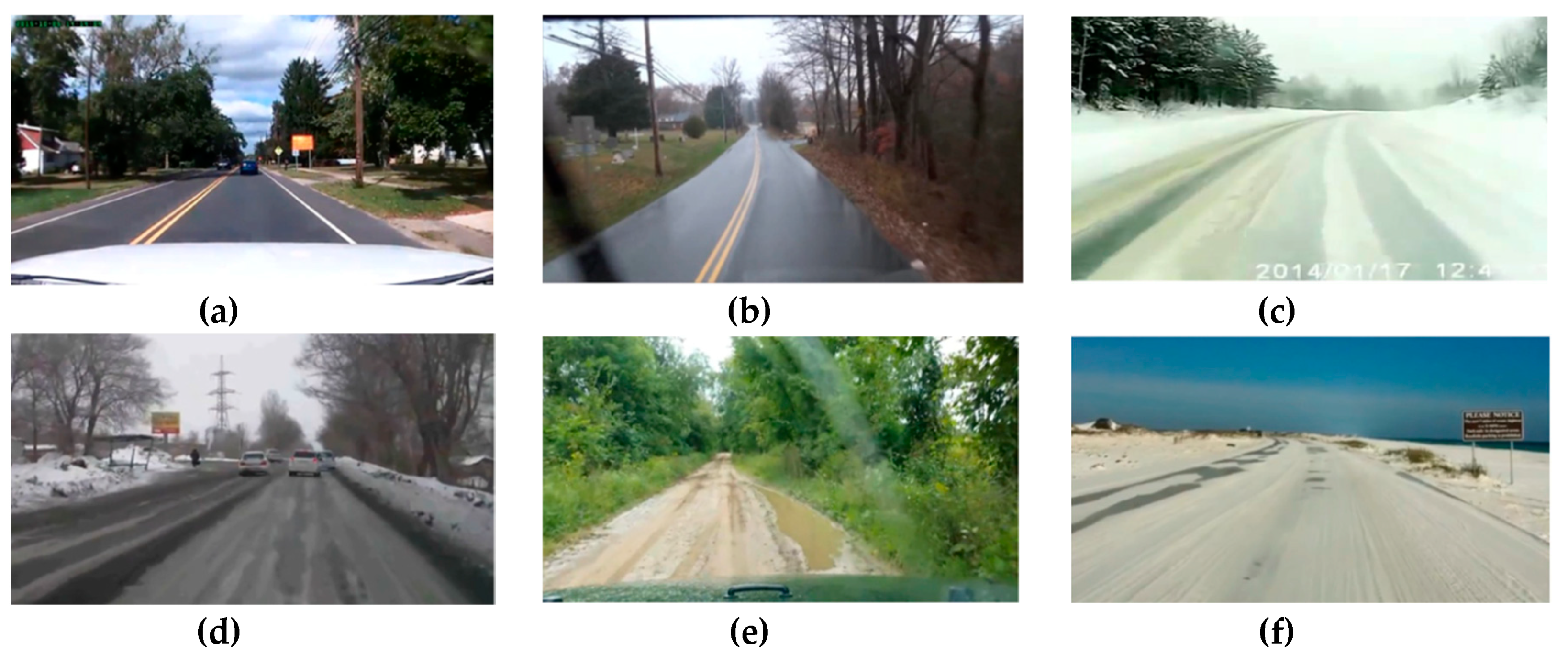
We used event data recorder video resources and other online video resources to collect our road surface condition images. Figure 7 shows sample images from this dataset. We collected 1200 images for our road surface condition dataset with six categories; each had 200 images. We split the dataset into 900 images (75%) for training and 300 images (25%) for testing.
The road surface condition dataset was created with six road surface conditions including dry, wet, snow, ice, puddle of water, and sand. The original images, as shown in Figure 7, contained information on the road surface and the surrounding background. The algorithm is designed for a forward-looking embedded vision sensor mounted on the rear-view mirror or dashboard. Only the area in front of the vehicle is of interest. The original images were divided into several blocks and only those road surface blocks of interest are extracted to create our road surface condition dataset. This sample image collection process helped us build a high-quality dataset for experiments.

3.2.1. Performance

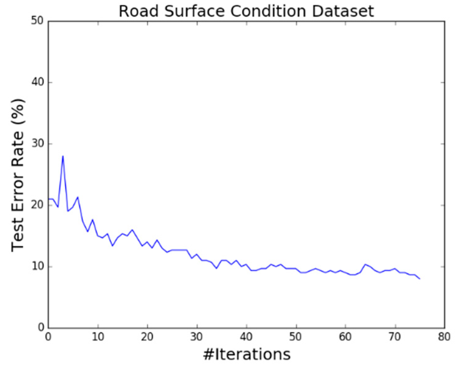
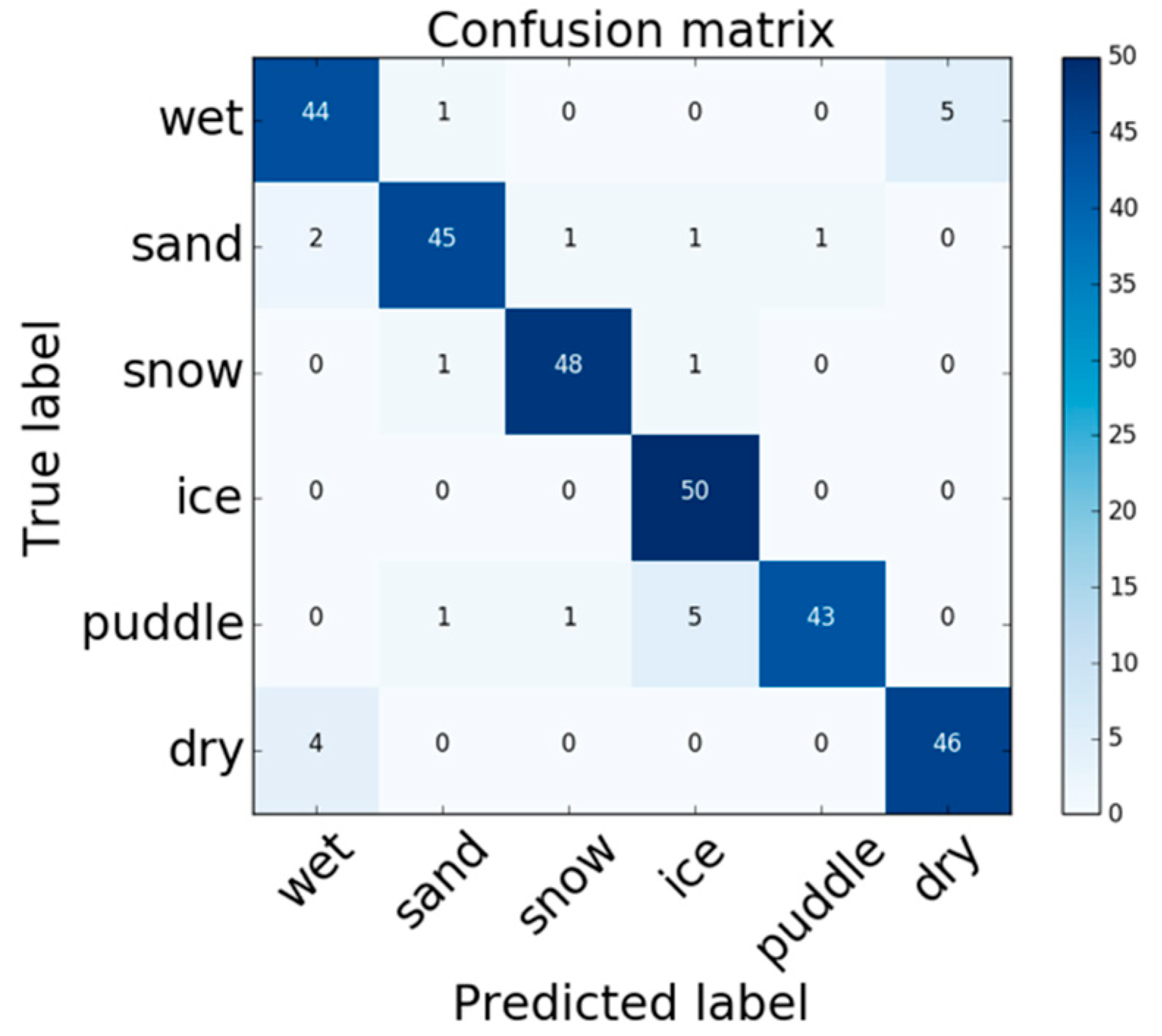
The proposed evolutionary algorithm obtained a 92% classification accuracy on our road surface condition dataset. For comparison, we also evaluated the boosted random forest method on this dataset without evolutionary learning. This simple random forest method obtained an 89.33% classification accuracy. This comparison demonstrated that our evolutionary learning method did discover useful features for classification. The classification performance of each iteration in the evolutionary learning on the road surface condition dataset is shown in Figure 8. It took the evolutionary learning algorithm approximately 40 learning iterations to reach its steady-state performance. The confusion matrix of the classification performance is shown in Figure 9. The dry and wet cases were easily confused because of the subtle differences between them. Ice and snow were the easiest to recognize. Whereas, puddle of water was the hardest because of its similarity with icy road surface.
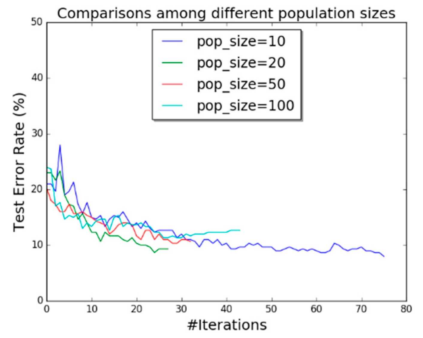
We also performed experiments using four different sizes of the population generated in the genetic algorithm. Figure 10 shows the performance comparison using different population sizes. It seems that using a relatively small population resulted in better performance. This is most likely because using a smaller population size allows for the exploration of those transform combinations which tend to mature more slowly than others but could eventually result in a higher fitness score. We ran the genetic algorithm in our evolutionary learning method using a population size of 10. The advantages of this population size are its computational efficiency and its ability to provide diversity in the learned features.

3.2.2. Visualization of Features from Evolutionary Learning

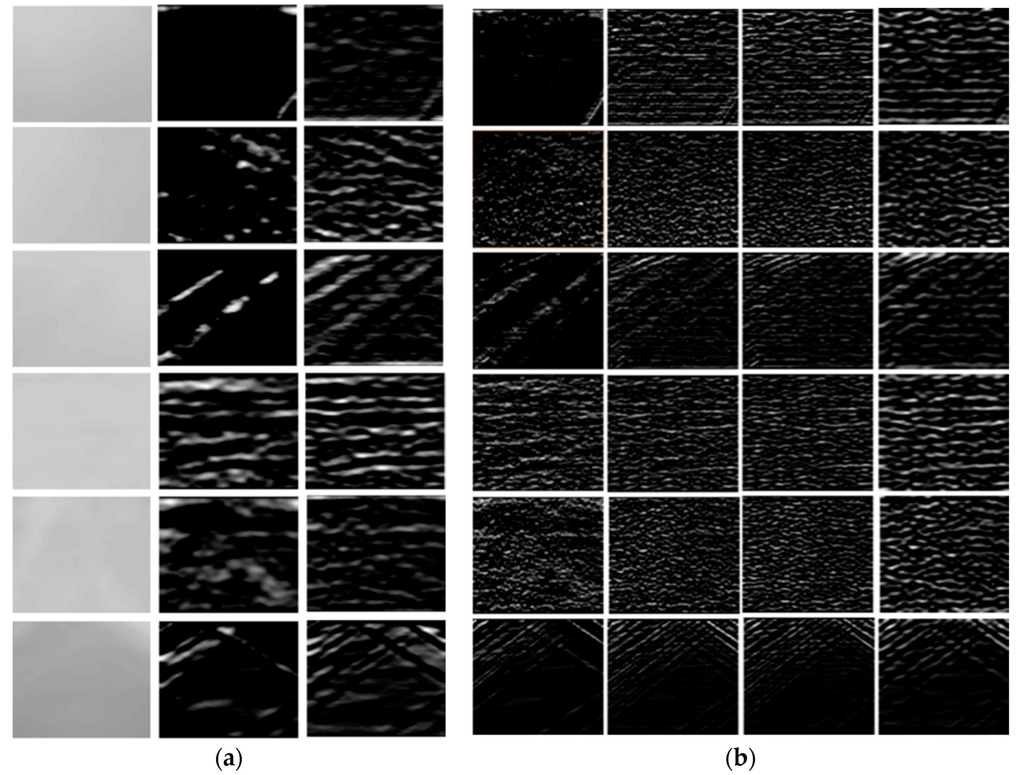
We took a closer look at the learned evolutionary image transformations or image features from our learning process. Specifically, we would like to visualize what the proposed method constructed for the road surface condition dataset. For visualization, we averaged the image transform outputs of all training images used for each specific class. The resulting average outputs were then normalized to be viewed as images. The output of each image transform in the learned transformation sequences was examined to show what information these transformations discovered.
As examples, Figure 11 shows two of thirty features learned from the road surface condition dataset. Each row represents a class of the road surface condition dataset which includes six road surface conditions including dry, wet, snow, ice, puddle of water, and sand (from top to bottom). Each column represents a particular transform that is used in that feature for all six classes. These transforms are shown in the order they appear in the feature from left to right. To be more specific, the first feature (Figure 11a) consists of three transforms, a Gaussian transform (Column 1), a Sobel transform (Column 2), and a Gradient transform (Column 3). The second feature (Figure 11b) consists of three Sobel transforms (Columns 1–3) and a Gaussian transform (Column 4).
As shown in Figure 11, texture is the most important piece of information that both features (Figure 11a,b) focus on extracting from the training images. Just like a human expert would rely heavily on texture information to classify these six classes, our evolutionary algorithm extracts image features that emphasize the image texture.

3.3. Pavement Quality Evaluation

Besides the road surface condition dataset, we also created a road pavement quality dataset to test our evolutionary algorithm. This dataset had four typical road pavement conditions including good pavement, line crack, net cracks, and potholes. These four conditions are the most common road pavement conditions in the real world. As with the road surface condition dataset, we also included 200 images for each pavement condition which gave us a total of 800 images in the road pavement condition dataset. Samples of this dataset are shown in Figure 12.

3.3.1. Performance

We carried out two experiments for pavement quality evaluation application. In the first experiment, we used our evolutionary learning algorithm on the road pavement condition dataset to evaluate its performance. Our classification accuracy on this dataset was 100%. The confusion matrix was not included because of perfect performance.
For the second experiment, we tested the boosted random forest method on the dataset without evolutionary learning to prove that our learning algorithm helps extract useful features for classification. We used boosting techniques on the raw image dataset without using any feature extraction methods. The classification accuracy dropped to 98.5%. Even though both methods performed well on the road pavement quality dataset, our evolutionary learning method was able to discover more useful features to obtain perfect classification accuracy.
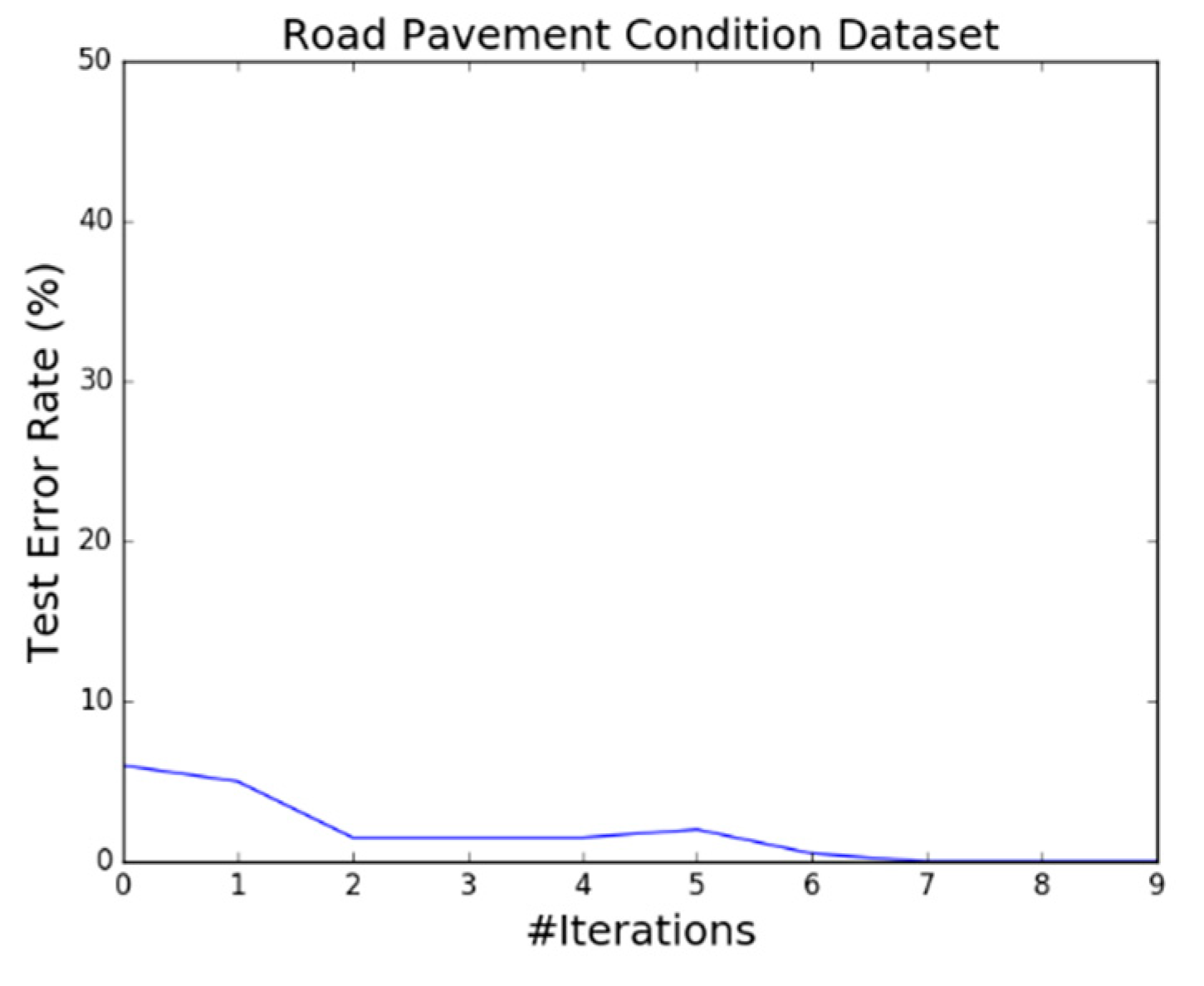
The classification performance of each iteration in the evolutionary learning on the road pavement quality dataset is shown in Figure 13. It took the algorithm only seven training iterations to reach 100% accuracy.

3.3.2. Visualization of Features from Evolutionary Learning

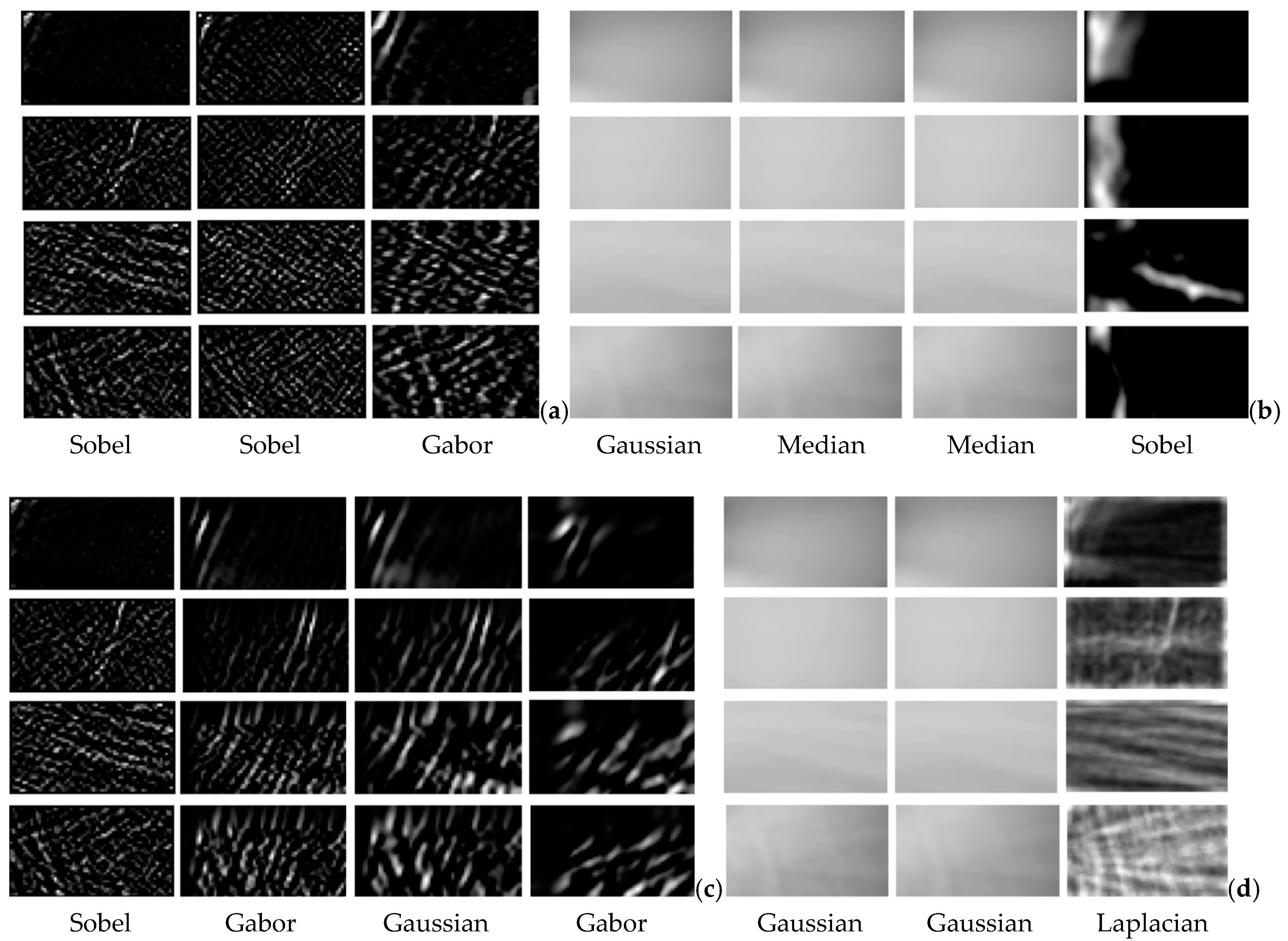
An approach for understanding and visualizing these evolutionary image transformations or image features obtained from our learning process was developed to interpret what the proposed method constructed for the road pavement quality dataset. The output of each image transform in the learned transformation sequences was examined to show what information these transformations discovered. For visualization, the image transform outputs of all training images used for each specific class were averaged and then normalized to be viewed as images.
Figure 14 shows four features learned from the road pavement condition dataset. This dataset had four pavement conditions. In Figure 14, each row represents a class of the road pavement condition dataset and each column represents a particular transform that was used to construct that feature for all four classes. These transforms are shown in the order they appear in the feature from left to right. The four features in Figure 14 have three or four transforms as a result of our evolutionary learning process. Both the first (Figure 14a) and the last (Figure 14d) features have three transforms. The second (Figure 14b) and the third (Figure 14c) features have four transforms. More specifically, the first feature consists of two Sobel transforms (Columns 1 and 2) and a Gabor transform (Column 3). The second feature consists of a Gaussian transform (Column 1), two Median Blur transform (Columns 2 and 3), and a Sobel transform (Column 4). The third feature consists of a Sobel transform (Column 1), a Gabor transform (Column 2), a Gaussian transform (Column 3), and a Gabor transform (Column 4). The last feature consists of two Gaussian transforms (Columns 1 and 2) and a Laplacian transform (Column 3). All these learned features have various transform sequences.
Like the features that were trained from the road surface condition dataset, the features shown in Figure 14 also indicate that the texture information was the most distinctive information being extracted from the images. Our model reached 100% classification accuracy with these features which shows a perfect classification performance on the dataset.

4. Conclusions

The aim of this work was to develop an efficient evolutionary algorithm specifically for embedded vision applications for visual inspection. The goal was to trade slight accuracy for processing efficiency in real-time performance. The proposed algorithm was not only capable of automatically learning global information from training images but also improving performance through the use of boosting techniques. The main advantage of the proposed method is its simplicity and computational efficiency, which makes it suitable for real-time embedded vision applications. We used 375, 104, 175, and 374 images for good, crack, dirt, and fertilized eggs, respectively, and 150 images for each class in both the road condition and pavement quality datasets for training. These are reasonably small numbers of images for data collection and training. The training time for our three example applications was 10 to 30 min on a PC depending on the number of iterations to reach steady-state performance. The processing speed was approximately 100 frames per second with an ARM processor running Linux, demonstrating its efficiency.
This algorithm accurately separated fertilized and unfertilized eggs and detected two common eggshell defects (i.e., dirt and crack). It distinguished six road surface conditions including dry, wet, snow, ice, puddle of water, and sand. It also recognized different road pavement qualities to detect cracks and potholes. For the three datasets created for the experiments, it obtained almost a perfect classification performance that is comparable to the performance obtained using other more sophisticated classification methods.
We recognize that these three sample applications might be viewed as straightforward cases and many other approaches could work just as well as the proposed method. As emphasized previously, our aim was to develop an efficient (fast and requiring very few training images) and easy-to-configure method that is versatile and does not depend on handcrafted features or manual tuning of parameters. These three applications clearly demonstrate the versatility of the proposed evolutionary learning algorithm and prove its suitability for real-time visual inspection applications that need to classify a small number of classes.
A hardware-friendly version of the algorithm was developed [32]. Our hardware simulation shows that the modifications and optimizations made to the algorithm for hardware implementation did not affect its performance. The hardware-friendly version was implemented in a field programmable gate array (FPGA) [32]. Our VHDL design can be used for building application-specific integrated circuits (ASICs) for applications that require a compact, low-cost, and low-power vision sensor.
Author Contributions

Conceptualization, M.Z. and D.-J.L.; Data curation, M.Z.; Formal analysis, Z.G.; Investigation, Z.G., M.Z. and D.-J.L.; Methodology, M.Z. and D.-J.L.; Project administration, D.-J.L.; Resources, Z.G. and D.-J.L.; Software, M.Z.; Validation, Z.G., M.Z. and D.-J.L.; Visualization, M.Z.; Writing—original draft, Z.G. and M.Z.; Writing—review and editing, D.-J.L.

Funding

This research was funded by the Small Business Innovation Research program of the US Department of Agriculture (#2015-33610-23786); the University Technology Acceleration Program (UTAG) of Utah Science Technology and Research (USTAR) (#172085) of the State of Utah, US; Technology Plan Project of Guangdong and the Innovation and Entrepreneurship project of university student of the Science, China (#2017A040405064 and #201821619083); and Major Scientific Research Projects of Guangdong Provincial Education Department (#2016KTSCX17).

Conflicts of Interest

The authors declare no conflict of interest. The funders had no role in the design of the study; in the collection, analyses, or interpretation of data; in the writing of the manuscript, or in the decision to publish the results.

References

  1. Motoda, H.; Liu, H. Feature selection, extraction and construction. Commun. Inst. Inf. Comput. Mach. 2002, 5, 67–72. [Google Scholar]
  2. Liu, H.; Motoda, H. Computational Methods of Feature Selection; Chapman and Hall/CRC Press: Boca Raton, FL, USA, 2007. [Google Scholar]
  3. Ferreira, A.J.; Figueiredo, M.A.T. An unsupervised approach to feature discretization and selection. Pattern Recognit. 2012, 45, 3048–3060. [Google Scholar] [CrossRef]
  4. Xue, B.; Zhang, M.; Browne, W.N.; Yao, X. A survey on evolutionary computation approaches to feature selection. IEEE Trans. Evol. Comput. 2016, 20, 606–626. [Google Scholar] [CrossRef]
  5. Krawiec, K.; Bhanu, B. Visual learning by evolutionary and coevolutionary feature synthesis. IEEE Trans. Evol. Comput. 2007, 11, 635–650. [Google Scholar] [CrossRef]
  6. Wang, X.; Yang, J.; Teng, X.; Xia, W.; Jensen, R. Feature selection based on rough sets and particle swarm optimization. Pattern Recognit. Lett. 2007, 28, 459–471. [Google Scholar] [CrossRef]
  7. Sun, Z.; Bebis, G.; Miller, R. Object detection using feature subset selection. Pattern Recognit. 2004, 37, 2165–2176. [Google Scholar] [CrossRef]
  8. Sherrah, J.R.; Bogner, R.E.; Bouzerdoum, A. The evolutionary pre-processor: Automatic feature extraction for supervised classification using genetic programming. In Proceedings of the Second Annual Genetic Programming Conference, Stanford, CA, USA, 13–16 July 1997; pp. 304–312. [Google Scholar]
  9. Pedergnana, M.; Marpu, P.R.; Mura, M.D.; Benediktsson, J.A.; Bruzzone, L. A novel technique for optimal feature selection in attribute profiles based on genetic algorithms. IEEE Trans. Geosci. Remote Sens. 2013, 51, 3514–3528. [Google Scholar] [CrossRef]
  10. Sia, F.; Alfred, R. Evolutionary-based feature construction with substitution for data summarization using DARA. In Proceedings of the 2012 4th Conference on Data Mining and Optimization (DMO), Langkawi, Malaysia, 2–4 September 2012; pp. 53–58. [Google Scholar]
  11. Mitchell, M. An introduction to genetic algorithms. Comput. Math. Appl. 1996, 32, 133. [Google Scholar]
  12. Espejo, P.G.; Ventura, S.; Herrera, F. A survey on the application of genetic programming to classification. IEEE Trans. Syst. Man Cybern. Part C Appl. Rev. 2010, 40, 121–144. [Google Scholar] [CrossRef]
  13. Tran, B.; Zhang, M.; Xue, B. Multiple feature construction in classification on high-dimensional data using GP. In Proceedings of the 2016 IEEE Symposium Series on Computational Intelligence (SSCI), Athens, Greece, 6–9 December 2016. [Google Scholar]
  14. Smith, M.G.; Bull, L. Genetic programming with a genetic algorithm for feature construction and selection. Genet. Program. Evolvable Mach. 2005, 6, 265–281. [Google Scholar] [CrossRef]
  15. Neshatian, K.; Zhang, M.; Johnston, M. Feature construction and dimension reduction using genetic programming. In Proceedings of the 20th Australian Joint Conference on Advances in Artificial Intelligence (AI’07), Gold Coast, Australia, 2–6 December 2007; Volume 4830, pp. 160–170. [Google Scholar]
  16. Ahmed, S.; Zhang, M.; Peng, L.; Xue, B. Multiple feature construction for effective biomarker identification and classification using genetic programming. In Proceedings of the 2014 Annual Conference on Genetic and Evolutionary Computation, Vancouver, BC, Canada, 12–16 July 2014; pp. 249–256. [Google Scholar]
  17. Lillywhite, K.D.; Tippetts, B.J.; Lee, D.J. Self-tuned Evolution-COnstructed features for general object recognition. Pattern Recognit. 2012, 45, 241–251. [Google Scholar] [CrossRef]
  18. Lillywhite, K.D.; Tippetts, B.J.; Lee, D.J.; Archibald, J.K. A feature construction method for general object recognition. Pattern Recognit. 2013, 46, 3300–3314. [Google Scholar] [CrossRef]
  19. Zhang, M.; Lee, D.J. Global ECO-Feature for object classification. In Proceedings of the International Symposium on Visual Computing, Las Vegas, NV, USA, 12–14 December 2016; Part II, LNCS 10073. pp. 281–290. [Google Scholar]
  20. Zhang, M.; Lee, D.J.; Lillywhite, K.D.; Tippetts, B.J. Automatic quality and moisture evaluations using evolution constructed features. Comput. Electron. Agric. 2017, 135, 321–327. [Google Scholar] [CrossRef]
  21. Mueller, M. Sensor Sensibility: Advanced Driver Assistance Systems; Vision Zero International: Geneva, Switzerland, 2015. [Google Scholar]
  22. Narayanan, B.; Beigh, K.; Loughnane, G.; Powar, N. Support vector machine and convolutional neural network based approaches for defect detection in fused filament fabrication. In Proceedings of the Applications of Machine Learning, San Diego, CA, USA, 23–27 August 2019; Volume 11139. [Google Scholar]
  23. Guo, X.; Singh, S.; Lee, H.; Lewis, R.; Wang, X. Deep learning for real-time Atari game play using offline Monte-Carlo tree search planning. In Proceedings of the 27th International Conference on Neural Information Processing Systems, Montréal, QC, Canada, 8–13 December 2014. [Google Scholar]
  24. Fernández-Delgado, M.; Cernadas, E.; Barro, S.; Amorim, D.; Amorim Fernández-Delgado, D. Do we need hundreds of classifiers to solve real world classification problems? J. Mach. Learn. Res. 2014, 15, 3133–3181. [Google Scholar]
  25. Li, T.; Ni, B.; Wu, X.; Gao, Q.; Li, Q.; Sun, D. On random hyper-class random forest for visual classification. Neurocomputing 2016, 172, 281–289. [Google Scholar] [CrossRef]
  26. Mishina, Y.; Murata, R.; Yamauchi, Y.; Yamashita, T.; Fujiyoshi, H. Boosted random forest. IEICE Trans. Inf. Syst. 2015, 98, 1630–1636. [Google Scholar] [CrossRef]
  27. Freund, Y.; Schapire, R.E. A decision-theoretic generalization of on-line learning and an application to boosting. J. Comput. Syst. Sci. 1997, 55, 119–139. [Google Scholar] [CrossRef]
  28. Schapire, R.E.; Singer, Y. Improved boosting algorithms using confidence-rated predictions. Mach. Learn. 1999, 37, 297–336. [Google Scholar] [CrossRef]
  29. Kégl, B.; Busa-Fekete, R. Boosting products of base classifiers. In Proceedings of the 26th Annual International Conference on Machine Learning, Montreal, QC, Canada, 14–18 June 2009; pp. 497–505. [Google Scholar]
  30. Hastie, T.; Rosset, S.; Zhu, J.; Zou, H. Multi-class AdaBoost. Stat. Interface 2009, 2, 349–360. [Google Scholar] [CrossRef]
  31. Seiffert, C.; Khoshgoftaar, T.M.; Van Hulse, J.; Napolitano, A. Resampling or reweighting: A comparison of boosting implementations. In Proceedings of the 20th IEEE International Conference on Tools with Artificial Intelligence, Dayton, OH, USA, 3–5 November 2008; Volume 1, pp. 445–451. [Google Scholar]
  32. Simons, T.S.; Lee, D.J. Jet Features: Hardware-friendly, learned convolutional kernels for high-speed image classification. Electronics 2019, 8, 588–607. [Google Scholar] [CrossRef] [Green Version]
Figure 1. Overview of the training procedure of the algorithm.
Electronics 08 01367 g001
Figure 2. (a) Egg candling and (b) backlight.
Electronics 08 01367 g002
Figure 3. Samples of egg images: (a) good, (b) crack, (c) dirt, and (d) fertilized.
Electronics 08 01367 g003
Figure 4. Confusion matrix of the classification results on the egg dataset.
Electronics 08 01367 g004
Figure 5. Classification performance of each evolutionary iteration on the egg dataset.
Electronics 08 01367 g005
Figure 6. Visualization of two features that were trained from the egg dataset.
Electronics 08 01367 g006
Figure 7. Samples of the road condition dataset: (a) dry, (b) wet, (c) snow, (d) ice, (e) puddle of water, and (f) sand.
Electronics 08 01367 g007
Figure 8. The classification error rate for each evolution iteration on the road surface condition dataset.
Electronics 08 01367 g008
Figure 9. The confusion matrix of the classification performance on the road surface condition dataset.
Electronics 08 01367 g009
Figure 10. Performance comparison among four different population sizes in the evolutionary learning on the road surface condition dataset.
Electronics 08 01367 g010
Figure 11. Visualization of features that are learned from the road surface condition dataset: (a) a feature that includes three transforms and (b) a feature that includes four transforms.
Electronics 08 01367 g011
Figure 12. Samples of the road pavement dataset: (a) good, (b) line cracks, (c) net cracks, and (d) potholes.
Electronics 08 01367 g012aElectronics 08 01367 g012b
Figure 13. The classification error rate for each evolution iteration on the road pavement quality dataset.
Electronics 08 01367 g013
Figure 14. Visualization of features that are learned from the road pavement condition dataset.
Electronics 08 01367 g014