Design and Analysis for Early Warning of Rotor UAV Based on Data-Driven DBN

Abstract

The unmanned aerial vehicle (UAV), which is a typical multi-sensor closed-loop flight control system, has the properties of multivariable, time-varying, strong coupling, and nonlinearity. Therefore, it is very difficult to obtain an accurate mathematical diagnostic model based on the traditional model-based method; this paper proposes a UAV sensor diagnostic method based on data-driven methods, which greatly improves the reliability of the rotor UAV nonlinear flight control system and achieves early warning. In order to realize the rapid on-line fault detection of the rotor UAV flight system and solve the problems of over-fitting, limited generalization, and long training time in the traditional shallow neural network for sensor fault diagnosis, a comprehensive fault diagnosis method based on deep belief network (DBN) is proposed. Using the DBN to replace the shallow neural network, a large amount of off-line historical sample data obtained from the rotor UAV are trained to obtain the optimal DBN network parameters and complete the on-line intelligent diagnosis to achieve the goal of early warning as possible as quickly. In the end, the two common faults of the UAV sensor, namely the stuck fault and the constant deviation fault, are simulated and compared with the back propagation (BP) neural network model represented by the shallow neural network to verify the effectiveness of the proposed method in the paper.

1. Introduction

The rotor UAV [1] is an aircraft that does not carry a pilot. It has been widely used in military and civilian fields for its unique advantages, so it is indispensable to ensure the safety and reliability of the rotor UAV flight control system. As an important device for information acquisition, the sensors [2] provide guarantees for the reliable safety of systems. Once faults occur, the flight safety of the rotor UAV will be affected, which will inevitably bring about system control performance degradation. Therefore, rapid detection of sensor failure [3] is a prerequisite for ensuring flight safety.

At present, for rotor UAV flight system sensors, the fault diagnosis method [4] is mostly model based [5], which [6] relies on the accurate model of the system [7]. However, owing to the improvement of computer capabilities, the advancement of artificial intelligence, and ultra-precision technology recently, the rotor UAV flight system has emerged an increasingly complex development trend, which is very difficult to obtain accurate mathematical models [8,9]. In contrast, the data-driven fault diagnosis method [10] has been proposed due to having no need for obtaining an accurate model of the system. The fault diagnosis can be completed only by using the input and output data of the system. Among them, the neural network method, which has self-association, self-adaptation, and no need to establish accurate mathematical models, are widely used in data-driven fault diagnosis methods. So far, researchers have used neural network methods to conduct extensive research on fault detection technology. The paper [11] presents a method of classifying impact noises obtained from a washer machine by obtaining the time frequency image of the sound signals, which is employed as the input signal to an artificial neural network classifier. A convolutional neural network, which is used to extract the residual signal from different sensor faults into the corresponding time-frequency map and fault characteristics to realize the diagnosis of the UAV sensor, is proposed in the literature [12]. From the visualization, the sensor failure information can be successfully constructed by the convolutional neural network (CNN) extracting the fault diagnosis logic between the residual and the health state. Reference [13] proposed wavelet packet threshold denoising and BP neural network methods for fault diagnosis of rolling bearings. In this method, the Levenberg–Maquardt algorithm was used to improve the traditional BP neural network, which greatly improves the diagnostic level. In reference [14], a novel data-driven adaptive neuron fuzzy inference system (ANFIS)-based approach was proposed to detect on-board navigation sensor faults in UAVs. The main advantages of this algorithm are that it allows the Kalman filter to estimate real-time model-free residual and ANFIS to build a reliable fault detection system. According to the experimental results, it was demonstrated that the method can not only detect fault quickly, but also can be used in real-time applications.

Nevertheless, the traditional shallow neural network method [15] has the disadvantages of over-fitting, local minimum, gradient attenuation, and poor generalization ability, which makes the effect of fault detection unsatisfactory [16].

Therefore, this paper proposes a deep learning method, deep belief network (DBN), instead of shallow neural network. As one of the classic algorithms for deep learning, DBN [17] solves problems such as dimension reduction, information retrieval, and fault classification successfully because of an excellent training algorithm and feature extraction. Therefore, it is applied to the field of fault diagnosis and has certain practicability.

In view of the above discussion, the fault diagnosis of rotor UAV flight control system sensor has been taken as an example and a fault diagnosis method for DBN is presented by this paper. By training a large number of offline historical sample data, the optimal network parameters obtained perform the feature extraction of fault and analyze more essential data features to make it easy to detect faults.

2. Mathematical Model of the Rotor UAV Flight Control System

2.1. Four-Rotor UAV Model

The Quadrotor AUV [18] is a system controlled by six degrees of freedom with strong coupling, nonlinearity, and interference sensitivity. The four rotors are symmetrically distributed in an “X” shape or a “十” shape, and the center of gravity of the rotor UAV is at geometric center. The power of the UAV is generated by four rotors [19], and the rotation of the rotor produces an upward lift, the magnitude of which is proportional to the square of the angular velocity of the rotor rotation$\mathrm{w}$, that is:

$$F_i=K{w}_i^2\hspace{1em}\hspace{1em}\hspace{1em}i=1,2,3,4$$

(1)

The Quadrotor AUV controls the attitude and position of the flight through four rotors. The two sets of rotors rotate in the opposite direction to counteract the anti-torsion moment to maintain the attitude stability. The total lift in the vertical direction is generated by four rotors [20], and the rotational speed difference of all the rotors produces the torque of horizontal direction to cause a yawing motion; the difference in rotational speed between the front and rear rotors controls the pitching motion; the left and right rotors controls the rolling motion [21]. The lift force are expressed as follows:

$$\begin{array}{l}{U}_z=F_1+F_2+F_3+F_4,\\ U_{\mathsf{\theta }}=bl\left(-F_2+F_4\right),\\ U_{\mathsf{\varphi }}=bl\left(F_1-F_3\right),\\ U_{\phi }=d\left(-F_1+F_2-F_3+F_4\right),\end{array}$$

(2)

where $b,d,l$ are respectively the rotor lift coefficient, the drag index, and the distance from the center of gravity to the axis of the quadrotor UAV$;U_z,U_{\mathsf{\theta }},U_{\mathsf{\varphi }},U_{\phi }$are respectively the total lift, rolling moment, pitching moment, and yawing moment of the rotor UAV [22]. Through the Newton–Eulerian formula, and assuming that the UAV is in slow flight or hover transition, the kinematics model is obtained. The results are as follows:

$$\begin{array}{l}\ddot{X}=\left(cos\mathsf{\varphi }sin\mathsf{\theta }cos\phi +sin\mathsf{\varphi }sin\phi \right)U_z/m,\\ \ddot{Y}=\left(cos\mathsf{\varphi }sin\mathsf{\theta }cos\phi +sin\mathsf{\varphi }sin\phi \right)U_z/m,\\ \ddot{Z}=g-\left(cos\mathsf{\varphi }cos\mathsf{\theta }\right)U_z/m,\\ \ddot{\mathsf{\varphi }}=\left(\ddot{\mathsf{\theta }\phi }\left(J_Y-J_Z\right)+U_{\mathsf{\theta }}\right)/J_X,\\ \ddot{\mathsf{\theta }}=\left(\ddot{\mathsf{\varphi }\phi }\left(J_Z-J_X\right)+U_{\mathsf{\varphi }}\right)/J_Y,\\ \ddot{\phi }=\left(\ddot{\mathsf{\theta }\mathsf{\varphi }}\left(J_X-J_Y\right)\right)/J_Z,\dots \end{array}$$

(3)

where $\ddot{X},\ddot{Y},\ddot{Z}$ are the accelerations of the rotor UAV in the ground coordinates and $\mathsf{\theta },\mathsf{\varphi },\mathsf{\phi }$are respectively the roll, pitch, and yaw of the four-rotor UAV. $m$ is the mass of the four-rotor UAV and $g$ is the acceleration of the UAV. $J_X,J_Y,J_Z$ are the moment of inertia of the$\mathrm{X}$shaft, $\mathrm{Y}$shaft, and $\mathrm{Z}$shaft.

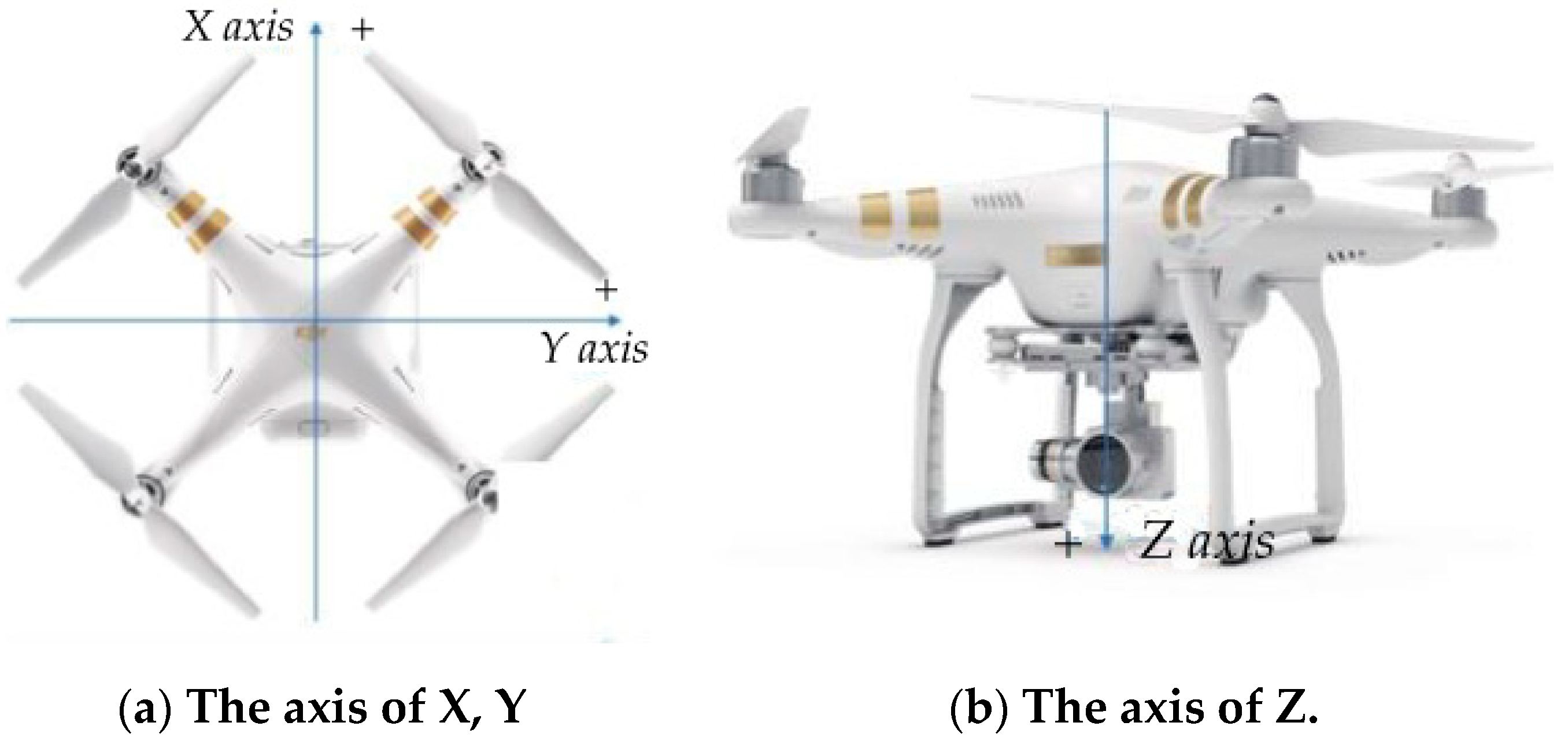
2.2. Flight Coordinate System Model

2.2.1. North East Coast Coordinate System

The Northeast coordinate system [23] is the geodetic coordinate system used by the DJI aircraft. Origin $O_g$is the take-off point. The three axes of the coordinate system are marked as the right north direction$O_g{X}_g$, the right east direction$O_g{Y}_g$, and the vertical ground direction$O_g{Z}_g$. In the attitude data packet, the north, east, and downward speed curves can be found. In these curves, the value is positive indicating that the speed is north, east, or down.

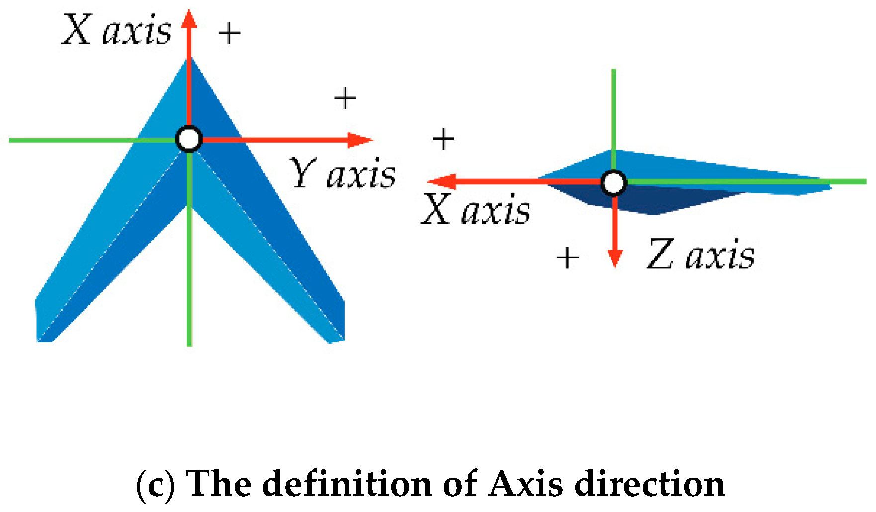
2.2.2. Aircraft Local Coordinate System

The aircraft center point $O_b$ is regarded as the coordinate origin in the aircraft local coordinate system. The three axes correspond to the front and back$O_b{X}_b$, left and right$O_b{Y}_b$, and up and down$O_b{Z}_b$ of the aircraft, respectively; positive and negative apply to the right hand screw rule, as shown in Figure 1.

2.2.3. Speed Coordinate Systems

The origin is taken at the center of gravity of the aircraft, and the axis $O_a{X}_a$ is in the same direction as the flight speed$\mathrm{V}$; the axis$O_a{Z}_a$is located on the vertical axis $O_a{X}_a$ of the plane of symmetry of the aircraft, pointing to the belly; $O_a{Y}_a$ is perpendicular to the plane$X_a{O}_a{Z}_a$, pointing to the right [24]. In the attitude data packet, the north, east, and downward speed curves can be found. In these curves, the value is positive indicating that the speed is north, east, or down.

2.2.4. Kinematic Equations for Angular Velocity

In order to describe the movement of the rotor UAV relative to the ground, the geometric relationship between the triaxial attitude angle [25] change rate and the three angular velocity components of the UAV is established as follows:

$$\begin{array}{l}\dot{\mathsf{\theta }}=p+qsin\mathsf{\theta }tan\mathsf{\varphi }+cos\mathsf{\theta }tan\mathsf{\varphi },\\ \dot{\mathsf{\varphi }}=qcos\mathsf{\theta }-rsin\mathsf{\theta },\\ \dot{\phi }=qsin\mathsf{\theta }/cos\mathsf{\varphi }+rcos\mathsf{\theta }/cos\mathsf{\varphi },\end{array}$$

(4)

where $p$ represents the rolling rate, $q$ represents the pitching rate, and $r$represents the yaw rate.

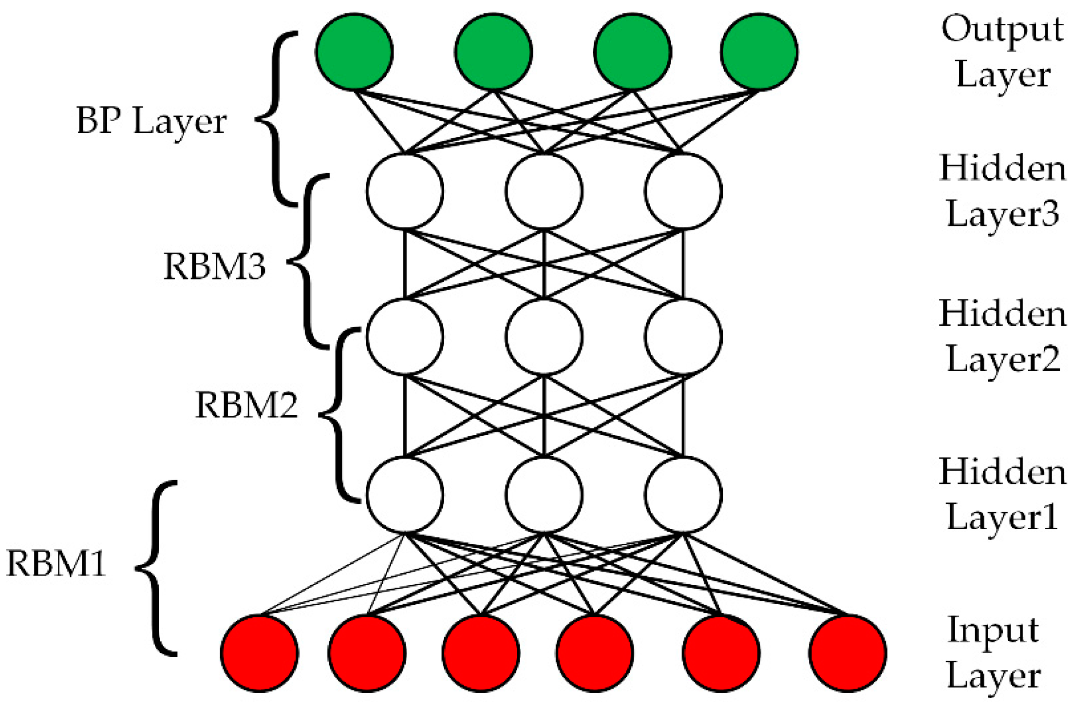
2.3. Deep Confidence Network Model

The deep learning idea [26] is inspired by the biological nervous system. It is made up of an input layer, multiple hidden layers, and an output layer. Each layer is connected to each other through nodes or neurons. The output of the previous layer is regarded as the input of each hidden layer. DBN, one of the classical algorithms for deep learning, can automatically extract low-level to high-level, concrete-to-abstract features [27] from raw data through a series of nonlinear transformations and is composed of a number of restricted Boltzmann machines (RBM) [28], which are commonly used to initially set the parameters of the feedforward neural network in order to improve the generalization ability of the model. The RBM network consists of$n$neurons and$m$hidden layer neurons. The connection between nodes exists only between layers. RBM comes from the classical thermal theory. The smaller the energy function is, the more stable the system is. The minimum energy of the network is trained to obtain the optimal parameters of the network. The energy function is expressed as follow:

$$\mathrm{E}\left(v,h\right)=-{\displaystyle \sum }_{i=1}^n{a}_i{v}_i-{\displaystyle \sum }_{j=1}^m{b}_j{h}_j-{\displaystyle \sum }_{i,j}{v}_i{h}_j{w}_{ij},$$

(5)

where $v_i,h_j$are respectively the random state of the$i$unit of the visible layer and the$j$ unit of the hidden layer; $a_i$ and$b_j$ are the corresponding bias; $w_{ij}$ are the weights between the two units. The purpose of training the network is to derive the optimal parameters $\left(w_{ij},a_i,b_j\right)$. The core is the process of using the layer-by-layer greedy learning algorithm to optimize the connection weight of the deep neural network, which firstly use the unsupervised layer-by-layer training method to effectively mine the fault features in the device to be diagnosed, and then add the corresponding classifier based through the way that reverse supervised fine-tuning to optimize the fault diagnosis capability of DBN. Some nonlinear complex functions can be learned from unsupervised layer-by-layer training by directly mapping data from input to output, which is the key to powerful feature extraction capabilities. Typical network structure [29] is shown in Figure 2.

3. Fault Diagnosis Method Based on Deep Confidence Network

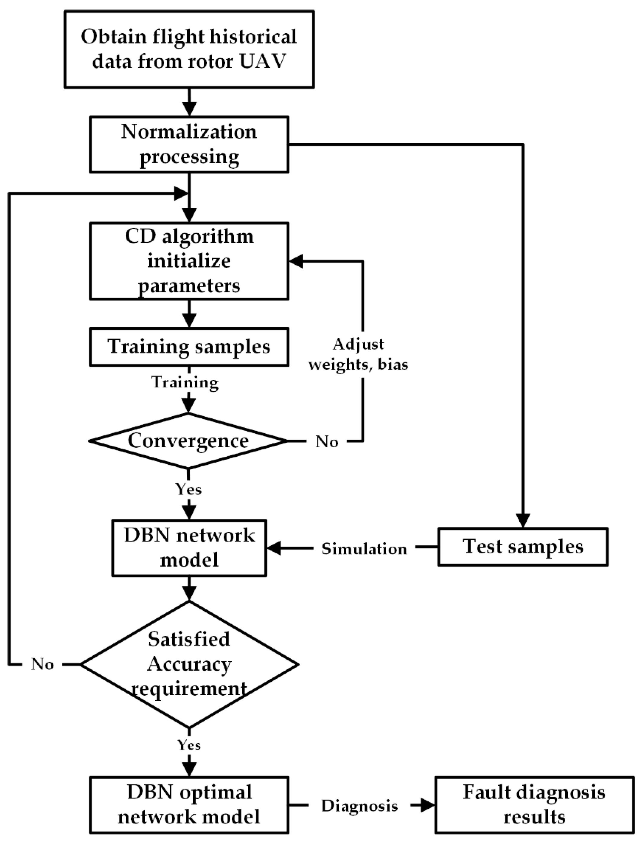
3.1. Off-Line Training Based on the DBN Model

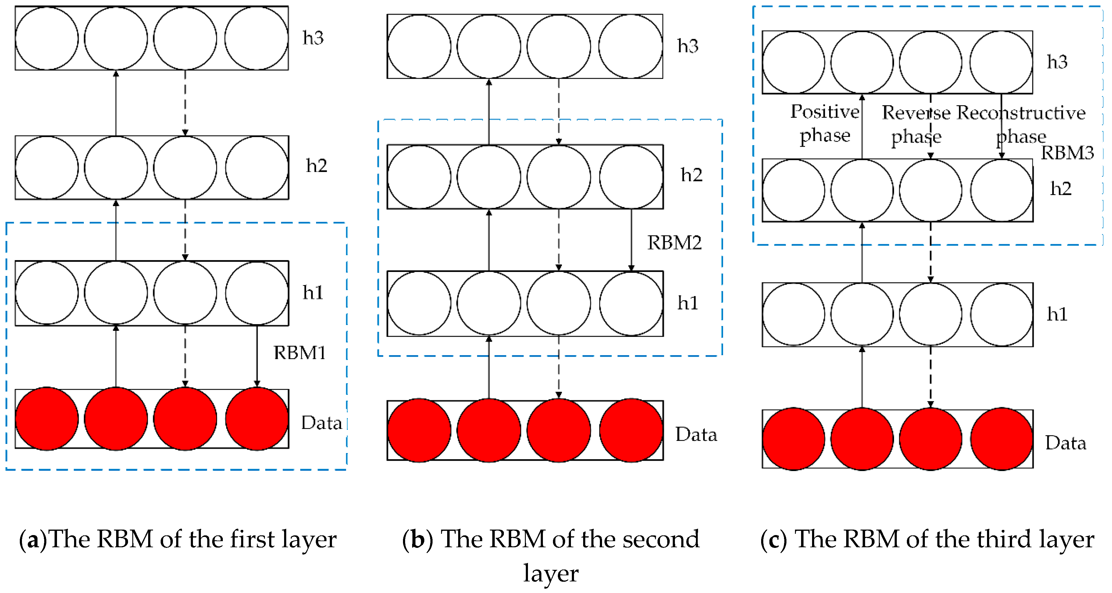
3.1.1. Deep Confidence Network Feature Extraction

Deep belief network, a self-learning feature extraction algorithm [30], has been widely used in many application fields with its powerful feature extraction capability [31] and participation without requiring a large amount of tag data. The process of DBN extracting fault features is shown in Figure 3.

The data layer is the visible layer and the initial input data. First, the data vector Data and the first layer hidden layer are used as the first RBM to train the weight $w$ and bias $a$ of the RBM, and then the parameters of the RBM are fixed;$\mathrm{h}1$ is regarded as the visible vector, and$\mathrm{h}2$ is treated as the hidden vector to train the second RBM to get its parameters, namely weight$w$ and bias$b$, and then fix these parameters; finally, to train RBM, which is composed of$\mathrm{h}1$ and$\mathrm{h}2$, the specific training algorithm is shown in Algorithm 1.

Algorithm 1. Description of RBM update algorithm.

This is the RBM update procedure for binomial units. It can easily adapted to other types of units.

$\mathrm{x}1$ is a sample from the training distribution for the RBM $\mathsf{\lambda }$ is a learning rate for the stochastic gradient descent in Contrastive Divergence $w$ is the RBM weight matrix, of dimension(number of hidden units, number of inputs) $a$ is the RBM offset vector for input units $b$ is the RBM offset vector for hidden units Notation: $\mathrm{Q}({\mathrm{h}}_2=1|{\mathrm{x}}_2)$ is the vector with elements $\mathrm{Q}({\mathrm{h}}_{2i}=1|{\mathrm{x}}_2)$  for all hidden units $i$ do   compute$\mathrm{Q}({\mathrm{h}}_{1i}=1|{\mathrm{x}}_1)$ (for binomial units, sigm($b_i+{\sum }_j{w}_{ij}{\mathrm{x}}_{1j}$))   sample ${\mathrm{h}}_{1i}ϵ\left\{0,1\right\}$ from $\mathrm{Q}({\mathrm{h}}_{1i}|{\mathrm{x}}_1)$  end for  for all visible units$j$ do   compute $\mathrm{P}({\mathrm{x}}_{2j}=1|{\mathrm{h}}_1)$ (for binomial units, sigm$\left(a_j+{\sum }_i{w}_{ij}{\mathrm{h}}_{1i}\right))$   sample ${\mathrm{x}}_{2j}ϵ\left\{0,1\right\}$ from $\mathrm{P}({\mathrm{x}}_{2j}=1|{\mathrm{h}}_1)$  end for  for all hidden units $i$ do   compute $\mathrm{Q}({\mathrm{h}}_{2i}=1|{\mathrm{x}}_2)$ (for binomial units, sigm$\left(b_i+{\sum }_j{w}_{ij}{\mathrm{x}}_{2j}\right))$  end for

$w\leftarrow w+\lambda \left({\mathrm{h}}_1{\mathrm{x}}_1^{\prime }-\mathrm{Q}\left({\mathrm{h}}_2=1{|\mathrm{x}}_2\right){\mathrm{x}}_2^{\prime }\right)$ $a\leftarrow a+\lambda \left({\mathrm{x}}_1-{\mathrm{x}}_2\right)$ $b=b+\lambda \left({\mathrm{h}}_1-\mathrm{Q}\left({\mathrm{h}}_2=1{|\mathrm{x}}_2\right)\right)$

3.1.2. Deep Confidence Network Training

In fact, the training of RBM is to find the probability distribution that produces the training samples well. Therefore, in order to eliminate the error caused by the data difference between different latitude and longitude, the original data need to be normalized.

$$\begin{array}{l}\mathrm{X}-=\mathrm{X}.\min ( ),\\ \mathrm{X}+=\mathrm{X}.\max ( ).\end{array}$$

(6)

The DBN learning and training process is mainly divided into two parts:

1. Unsupervised pre-training based on restricted Boltzmann machines from the bottom to the top.

Since the deep belief network is a neural network based on probability model, the decisive factor of its probability distribution depends on the weight $w$, so the goal of the training is to find the best weight. The contrastive divergence (CD) algorithm that finds the best weight is to randomly initialize the parameter set of RBM [32] $w_{ij},a_i,b_j$. Among them, $a_i$ is the bias of the$i$node of the visible layer;$b_j$ is the bias of the$j$ node of the hidden layer;$w_{ij}$ is the connection weight of the$i$ node of the visible layer; and the$j$ node of the hidden layer. $\langle {\rangle }_{recon}$ is a reconstructed sample obtained by sampling Gibbs to the sample to estimate the expectation. The learning algorithm is as follows, in Equation (7). Simultaneously, the description of the CD-k algorithm and train unsupervised DBN algorithm are expressed in Algorithms 2 and 3, respectively.

$$\begin{array}{r}\mathsf{\Delta }{w}_{ij}=\lambda \left(\langle v_i{h}_j{\rangle }_{data}-\langle v_i{h}_j{\rangle }_{recon}\right),\\ \mathsf{\Delta }{a}_i=\lambda (\langle v_i{\rangle }_{data}-\langle v_i{\rangle }_{recon}),\\ \mathsf{\Delta }{b}_j=\lambda (\langle h_j{\rangle }_{data}-\langle h_j{\rangle }_{recon}),\end{array}$$

(7)

Algorithm 2. CD-k algorithm description.

Input:$\mathrm{RBM}$($V_1,\dots ,V_n,H_1,\dots ,H_m$), training batch $\mathrm{S}$ Output: gradient approximation $\mathsf{\Delta }{w}_{ij},\mathsf{\Delta }{a}_i\mathrm{and}\mathsf{\Delta }{b}_j$ for $i=1,\dots ,n;j=1,\dots ,m$.

1  initialize $\mathsf{\Delta }{w}_{ij}=\mathsf{\Delta }{a}_i=\mathsf{\Delta }{b}_j=0$ for $i=1,\dots ,n;j=1,\dots ,m$ 2    for all the $vϵS$ do 3    $v^{\left(0\right)}\leftarrow v$ 4    for $t=0,\dots ,k-1$ do 5     for $i=1,\dots ,n$ do sample $h_i^{\left(t\right)}\sim p(h_i|v^{\left(t\right)})$ 6     for $j=1,\dots ,m$ do sample$v_j^{\left(t+1\right)}\sim p(v_j|h^{\left(t\right)})$ 7    for $i=1,\dots ,n;j=1,\dots ,m$ do 8    $\mathsf{\Delta }{w}_{ij}\leftarrow \mathsf{\Delta }{w}_{ij}+p\left(H_i=1|v^{\left(0\right)}\right)·v_j^0-p\left(H_i=1|v^{\left(k\right)}\right)·v_j^{\left(k\right)}$ 9    $\mathsf{\Delta }{a}_i\leftarrow \mathsf{\Delta }{a}_i+v_j^{\left(0\right)}-v_j^{\left(k\right)}$ 10    $\mathsf{\Delta }{b}_j\leftarrow \mathsf{\Delta }{b}_j+p\left(H_i=1|v^{\left(0\right)}\right)-p\left(H_i=1|v^{\left(k\right)}\right)$

Algorithm 3. Description of the train unsupervised DBN algorithm.

Train a DBN in a purely unsupervised way, with the greedy layer-wise procedure in which each added layer is trained as an RBM.

$\widehat{P}$ is the input training distribution for the network $\mathsf{\lambda }$ is a learning rate for the RBM training $\mathsf{\eta }$ is the number of layers to train $w^k$ is the weight matrix for $k$, for$k$ from 1 to $\mathsf{\eta }$ $a^k$ is the visible units offset vector for RBM at level $k$, for$k$ from 1 to $\mathsf{\eta }$ $b^k$ is the hidden units offset vector for RBM at level$k$, for$k$ from 1 to $\mathsf{\eta }$ Mean_field_computation is Boolean that is true if training data at each additional level is obtained by a mean-field approximation instead of stochastic sampling  for $k=1$ to $\mathsf{\eta }$ do   initialize $w^k=0,a^k=0,b^k=0$   while not stopping criterion do     sample ${\mathrm{h}}^0=\mathrm{x}$ from $\widehat{P}$     for $i=1$ to $k-1$ do      if mean_field_computation then       assign ${\mathrm{h}}_j^i$ to $\mathrm{Q}({\mathrm{h}}_j^i=1|{\mathrm{h}}^{i-1})$, for all elements $j$ of ${\mathrm{h}}^i$      else       sample ${\mathrm{h}}_j^i$ from ${\mathrm{Q}(\mathrm{h}}_j^i|{\mathrm{h}}^{i-1})$, for all elements$j$ of ${\mathrm{h}}^i$      end if     end for      RBMupdate$({\mathrm{h}}^{k-1},\lambda ,W^k,a^k,b^k)$ {thus providing $\mathrm{Q}({\mathrm{h}}^k|{\mathrm{h}}^{k-1})$ for future use}  end while end for

The CD algorithm is used to train layer by layer for DBN, obtaining the parameters of each layer and initializing the DBN, and then fine-tuning the parameters with the supervised learning algorithm.

2. Supervised tuning training from the top to the bottom.

For supervised tuning training, the forward propagation algorithm is used to obtain a certain output value from the input firstly, and then the backward propagation algorithm is used to update the weights and bias values of the network.

• Forward Propagation Algorithm

1. Pre-trained $w,b$ with the CD algorithm to determine the opening and closing of the corresponding hidden elements. Calculating the stimulus values for each hidden element are as follows:

$$h^{\left(l\right)}=w^{\left(l\right)}·v+b^{\left(l\right)}$$

(8)

where $l$ is the layer index of the neural network. The values of $w$ and $b$ are as follows:

$$w=\left[\begin{array}{ll}\begin{array}{ll}\begin{array}{ll}{w}_{1,1}& w_{2,1}\\ w_{1,2}& w_{2,2}\end{array}& \begin{array}{l}\dots \\ \dots \end{array}\\ \begin{array}{ll}\dots & \dots \end{array}& \dots \end{array}& \begin{array}{l}{w}_{n,1}\\ \begin{array}{l}{w}_{n,2}\\ \dots \end{array}\end{array}\\ \begin{array}{lll}{w}_{1,m}& w_{2,m}& \dots \end{array}& w_{n,m}\end{array}\right],b=\left[\begin{array}{l}{b}_1\\ b_2\\ \begin{array}{l}\dots \\ b_m\end{array}\end{array}\right],$$

(9)

where $w_{i,j}$ represents the weight from the$i$ explicit element to the$j$hidden element.

2. Spread out layer by layer, calculate the excitation value of each hidden element in the hidden layer layer by layer, and standardize it with sigmoid function, as shown below:

$$\mathsf{\sigma }{\left(h_j\right)}^{\left(l\right)}=\frac{1}{1+e^{-h_j}}.$$

(10)

3. Finally, the excitation value and output of the output layer are calculated as follows:

$$\begin{array}{c}{h}^{\left(l\right)}=w^{\left(l\right)}·h^{\left(l-1\right)}+b^{\left(l\right)},\\ \widehat{X}=f\left(h^{\left(l\right)}\right),\end{array}$$

(11)

where $f(·)$ represents the activation function of the output layer and the output value of the output layer is $\widehat{X}$.

• Back Propagation Algorithm

1. The error back propagation algorithm of the reconstruction error criterion is used to update the parameters of the whole network and evaluate whether the RBM is trained in the paper. The reconstruction error is the difference between the training data and the original data after the Gibbs sampling by RBM, as shown below:

$$\mathrm{J}={\sum }_{k=1}^n\Vert v-v^{\left(k\right)}\Vert .$$

(12)

The reconstruction error is continuously reduced by iteration times until all RBM training is completed. Finally, the global fine-tuning is performed. Since the last layer of the deep confidence network is used for parameter fitting, the activation function of the last layer selects the hyperbolic tangent function, namely:

$$f\left(x\right)=1-1/\left(1+e^{2x}\right).$$

(13)

The output value of the network between −1 and 1 is made. The process of fine-tuning the deep belief network parameters is the process of tuning using the back propagation algorithm. Given the input and output samples, the gradient descent algorithm is used to update the network weights and bias parameters as follows:

$$\left(w^l,b^l\right)\leftarrow \left(w^l,b^l\right)-\lambda ·\frac{\partial E}{\partial \left(w^l,b^l\right)},$$

(14)

where $\lambda$ is the learning rate whose numerical value represents the step size of each parameter adjustment. It is generally between 0.005 and 0.200, where $\lambda =0.10$. In order to overcome the problem that the training process easily falls into the local minimum value, the impulse term is introduced, and the parameter update direction is inconsistent with the gradient direction. The method is as follows:

$$w_{ij}^{t+1}=m{w}_{ij}^t+\lambda \frac{{\partial }_{\mathsf{\theta }}}{\partial w_{ij}},$$

(15)

where$m$ is the momentum term, where $m=0.5$; $t$ is the number of iterations for the sample.

3.2. Objective Function Establishment of DBN Fault Diagnosis Model

The deep belief network model is essentially a mapping relationship between input data and output data, that is,

$$\begin{array}{l}{\mathsf{\theta }}_x=f\left(H_{x-1},{\dot{H}}_{x-1},W_x,p_x,q_x,{\mathsf{\varphi }}_x,{\mathsf{\theta }}_{x-1}\right),\\ {\mathsf{\varphi }}_x=f\left(H_{x-1},{\dot{H}}_{x-1},W_x,q_x,r_x,{\mathsf{\theta }}_x,{\mathsf{\varphi }}_{x-1}\right),\\ {\phi }_x=f\left(H_{x-1},{\dot{H}}_{x-1},W_x,q_x,r_x,{\mathsf{\theta }}_x,{\phi }_{x-1}\right),\end{array}$$

(16)

where $H$ stands for the flight height of the aircraft; $\dot{H}$ expresses the rate of change of altitude;$W$ expresses the wind speed.

3.3. Online Diagnosis Based on the DBN Model

After the offline training of the deep confidence network is completed, the online estimation can be performed, and the residual between the estimated value and the real value is used to judge whether the fault is faulty. The residual at a certain moment is specifically described as follows:

$$\mathrm{e}\left(\mathrm{t}\right)=\tilde{o}\left(t\right)-o\left(t\right).$$

(17)

The detection threshold$K_t$ is set for each parameter sensor. By comparing the residual and the threshold, we can determine if there is a fault. When $\left|e\left(t\right)\right|<Kt$, it is judged to be faultless; when $\left|e\left(t\right)\right|\ge Kt$, it is determined to be faulty. The value of $K_t$ depends on the specific parameters as the case may be. The sensor output value can intuitively determine the stuck fault within a certain period of time, but other sensor fault types such as the constant deviation fault needs to satisfy the mathematical expression of the unknown fault type, as follows:

$$Y_{\left(t\right)}=k{y}_{\left(t\right)}+a,t\ge T$$

(18)

where $k$ is the failure factor, $a$ is the deviation, and $t$ is the time at which the failure occurred.

Different fault types correspond to different parameters $k$ and $a$ in Equation (18). In the case of a fault within a certain period of time, the DBN estimated value ${\tilde{y}}_{\left(t\right)}$ is used instead of the true value $y_{\left(t\right)}$ in Equation (18), that is:

$$Y_{\left(t\right)}=k{\tilde{y}}_{\left(t\right)}+a,t\ge T.$$

(19)

As long as the values of the parameters $\mathrm{k}$ and $\mathrm{a}$ are known and the estimated values $\tilde{k}$ and $\tilde{a}$ are obtained by a function fitting, the category of the fault can be distinguished. The specific fault type and parameter are as follows in

Table 1. Corresponding of fault type and parameter.

Fault Type	Parameter
Constant deviation fault	$\mathrm{k}=1,\left|\mathrm{a}\right|\ge K_t$
Constant gain fault	$\mathrm{k}\ne 1,\left|\mathrm{a}\right|<K_t$

.

When the sensor fault is detected by the deep confidence network, the signal reconstruction should be taken in time; that is, the output signal of the sensor is disconnected, and the output of the sensor is replaced by the output estimated by the DBN to ensure that the aircraft continues to fly safely.

4. Experiment and Analysis

4.1. Experimental Platform

The experiment is run on the Windows Operating System, which is configured as Intel Core i7, 16G memory. The encoding is done on the PyCharm platform that include the TensorFlow Framework. By comparing the model of the traditional BP neural network and the DBN network in the paper, the results will be analyzed accordingly.

The data used in this experiment are derived from the DJI four-rotor UAV. The data in the rotor UAV flight control data record mainly consist of eight parts, namely attitude data, on-screen display (OSD) data, controller data, remote control data, motor data, motor governor data, battery data, and obstacle avoidance data. The data are collected mainly from the attitude data as the source of experimental data in the paper. The attitude data mainly include information on sensors such as position, velocity, angular velocity, accelerometer, gyroscope, magnetometer, barometer, and so on.

The flight data are obtained from the flight attitude data of the rotor UAV. Via the process of normalization, the training samples and the test samples are established. First, the training samples are used for model training, and the weight and bias are continuously adjusted to make it converge quickly, and then the test samples is tested for the fault diagnosis effect to obtain the optimal DBN model. The fault diagnosis process is shown in Figure 4. When collecting data [33], data obtained in various flight state as much as possible, including altitude, altitude change rate, wind speed, pitch, yaw, roll pitch rate, yaw rate, and roll rate. When collecting training data, the flight altitude is 200 m, the flight speed is 40 m/s, the sampling time is 600 s, and the sampling period is 0.1 s.

4.2. Model Evaluation Index Determination

In order to better analyze the model in the paper, root mean square error (RMSE) and coefficient of determination (R2) are used for the index of regression evaluation. The description is defined as follows.

4.2.1. The Description of the RMSE

RMSE is a measure that reflects the degree of difference between predicted value and actual value. The larger the value is, the larger the difference is. The formula is as follows:

$$\mathrm{RMSE}\left(y_i,\widehat{y_i}\right)=\sqrt{\frac{1}{n}{\displaystyle \sum }_{i=1}^n{\left(y_i-\widehat{y_i}\right)}^2},$$

(20)

where $n$ is the dimension of the sequence,$\widehat{y_i}$ represents the prediction value of sensor angular rate, and $y_i$ represents the actual value of sensor angular rate.

4.2.2. The Description of the R2

R2 is also called the goodness of fit. The larger the goodness of fit, the denser the observation point is near the regression line. R2 is in the range between 0 and 1. The larger the value, the better the prediction effect. The expression formula is as follows:

$$R^2\left(y_i,\widehat{y_i}\right)=1-\frac{{\sum }_{i=1}^m{\left(y_i-\widehat{y_i}\right)}^2}{{\sum }_{i=1}^m{\left(y_i-\overline{y_i}\right)}^2},$$

(21)

where $\overline{y_i}$ is expressed as the average value of sensor angular rate.

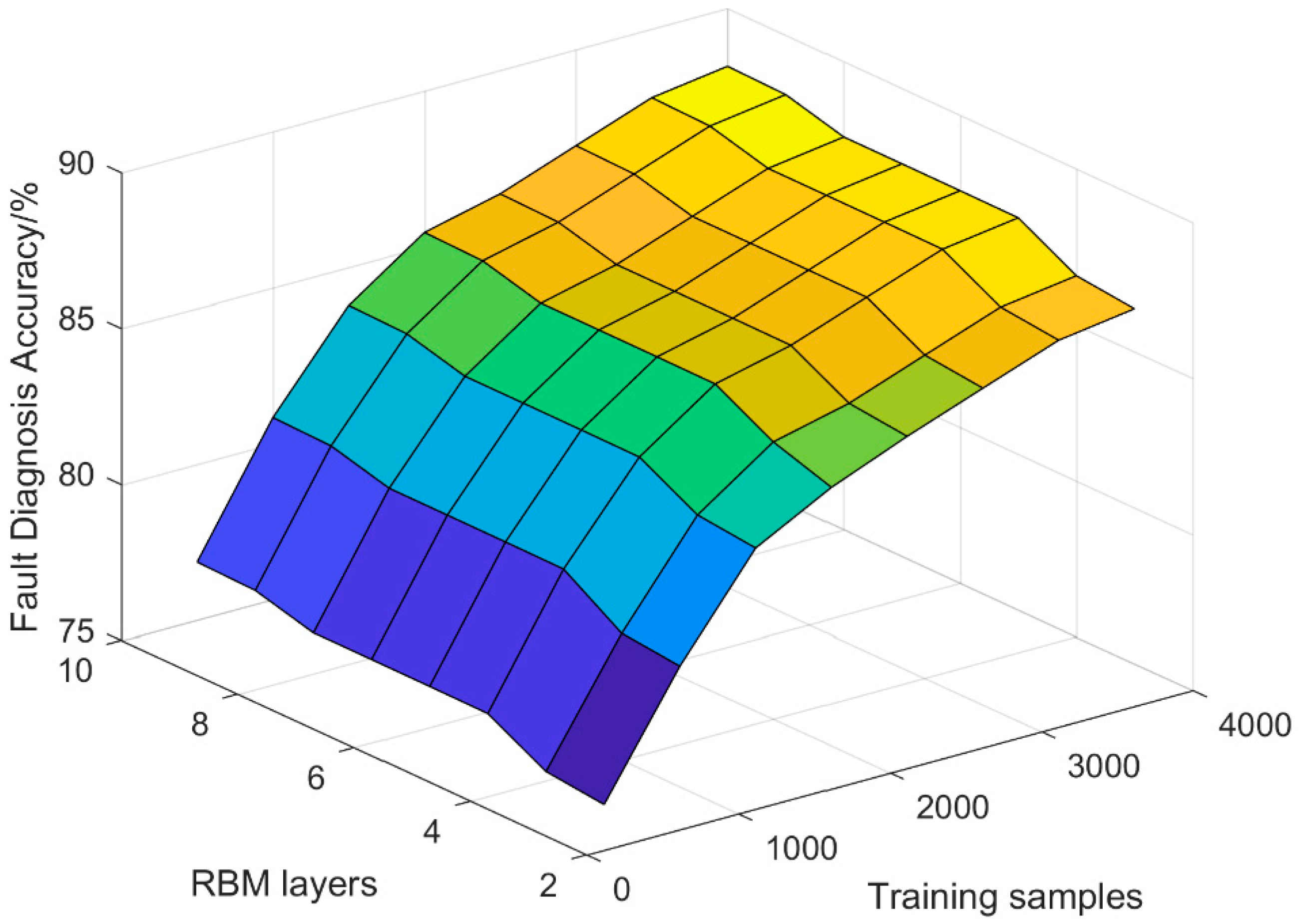
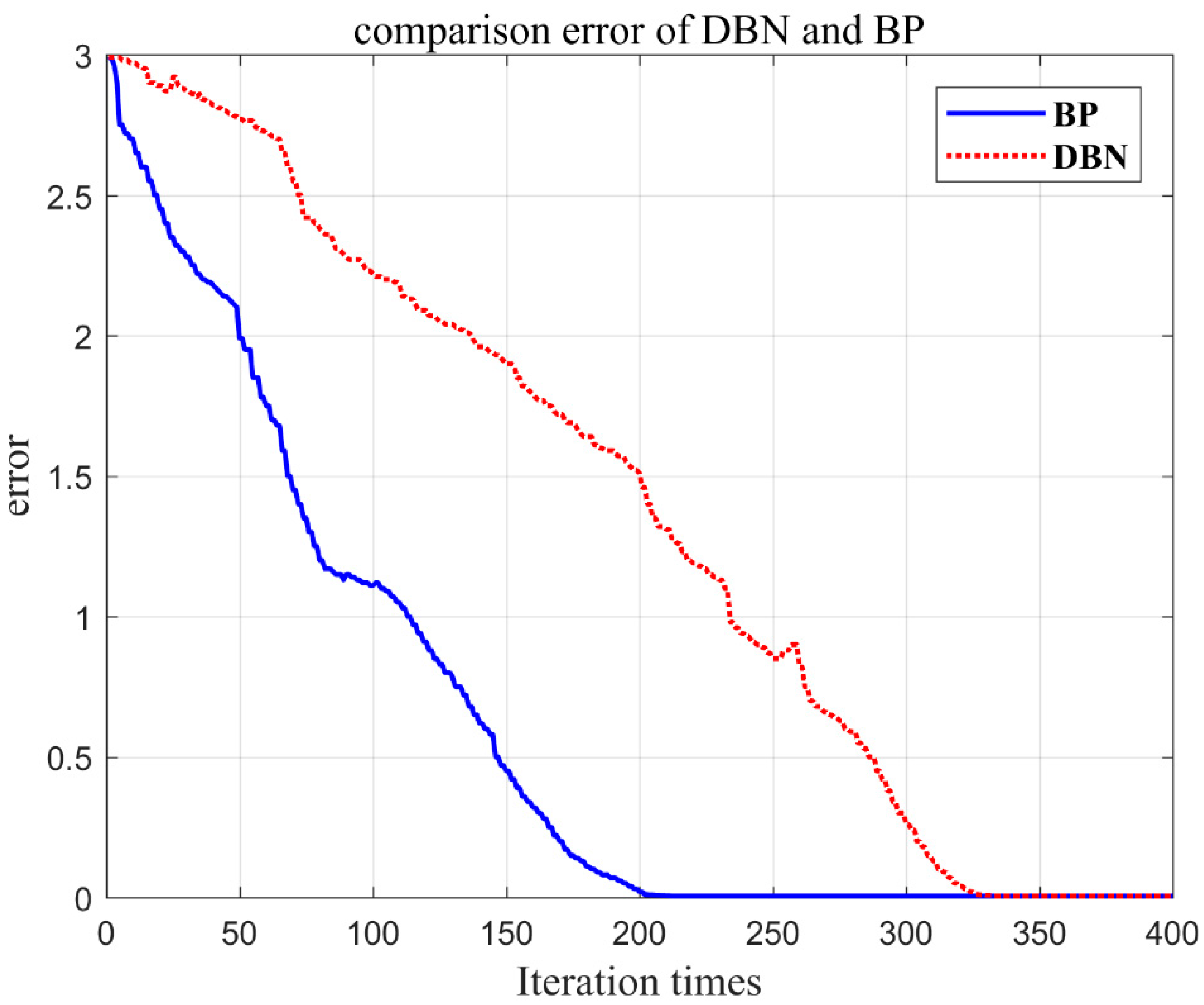
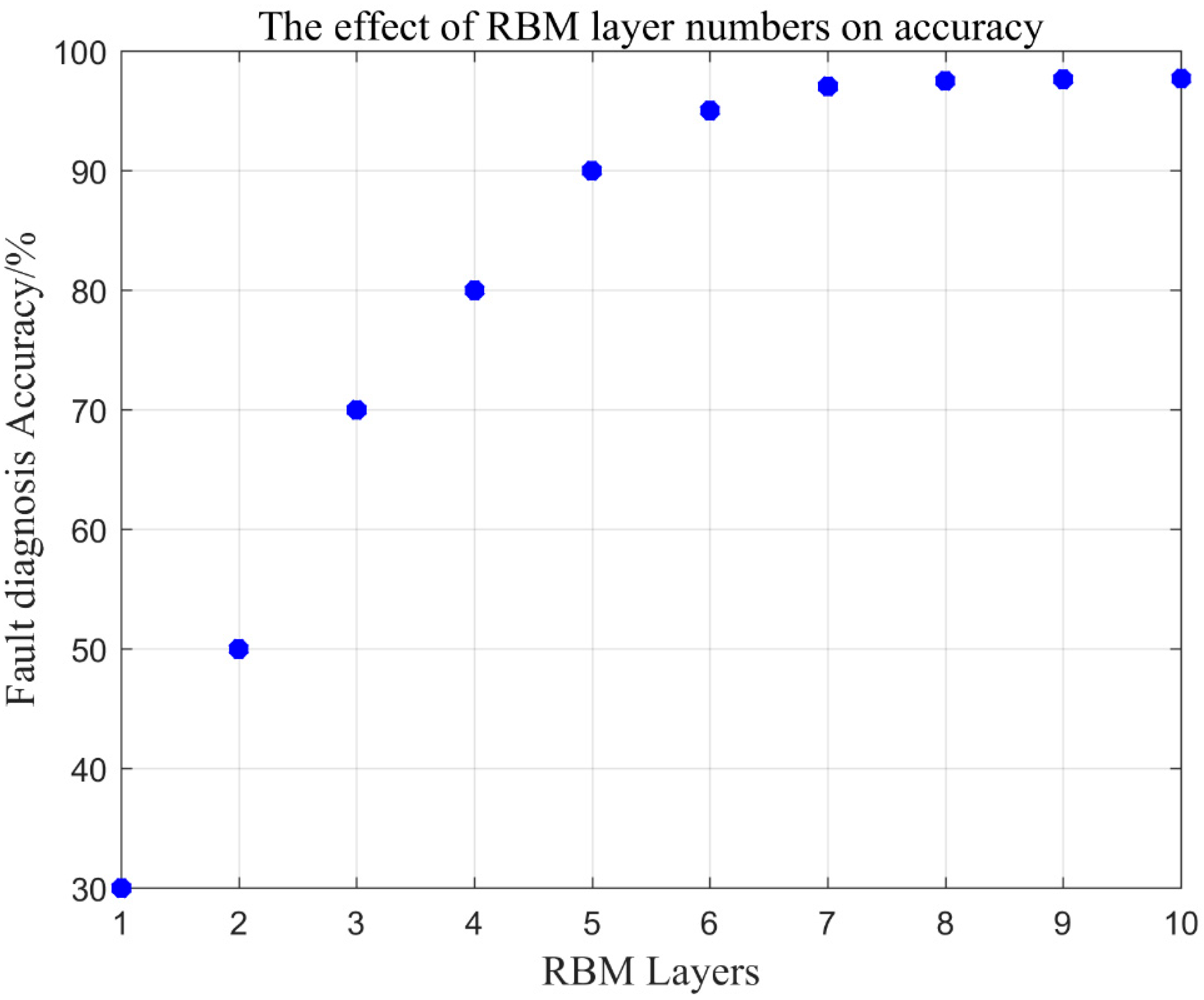
4.3. Model Structure Selection and Training Results

In the testing, the accuracy of fault diagnosis has a certain relationship with the training samples and the number of RBM layers in the network. When the training samples is different, the RBM layers of the network will also change accordingly. The relationship between the three variables is shown in Figure 5. Firstly, the underlying RBM is constructed with a network model of 3 to 10 layers. The number of neurons in the middle layer is initialized by the random number between 10 and 100. After an overwhelming number of training tests, the iteration times and the reconstruction error convergence curve are as shown in Figure 6.

As can be seen from Figure 6, in the initial stage, as the number of iteration times increases, the reconstruction error decreases rapidly. When the number of iteration time is greater than 200 times, the error reduction gradually stabilizes. Therefore, the number of RBM iteration time per layer is set to 200. On the premise that the training samples is fixed and the number of RBM iterations per layer is set to 200, the diagnostic accuracy of different RBM layers is tested. Change the number of RBM layers, starting at level 0 and modeling only the top level classifier until level 10. The correct relationship diagram is shown in Figure 7.

Figure 7 shows that with the increase of RBM layers, the accuracy of fault dignosis is on the rise, and the trend gradually becomes slow. When the RBM is 0 layer, the classification result has the lowest correct rate, only 30%. As the number of layers increases, the discriminative performance of the model increases continuously. However, when the effect of seven layers is reached, the correct rate curve almost no longer rises. The number of bottom RBM layers is six layers and it has reached 95% or more, so the number of RBM layers of the selected model is six layers. Lastly, using the roll sensor, the yaw sensor, and the pitch sensor under normal working conditions, the shallow neural network BP [34] is compared with the deep neural network DBN proposed in the paper, as shown in Figure 8, Figure 9 and Figure 10.

In Figure 8, it can be seen that at 22 s of flight time (x = 22), the flying hand hits about 2% of the crossbar (y = −2.1°) to the left. Then, it leaned to the right again. Corresponding to the actual flight situation, the flying hand went to the left and rolled the bar, but it was released again. According to this situation, the DBN model proposed in this paper can respond well to the stroke situation and has a strong generalization ability.

As can be seen in the trend of the curve in Figure 9, the aircraft yaw is −68° (y = −68°) at 9 s of flight time (x = 9). Nevertheless, at about 10 s, the yaw changes and the value increases from small to large, indicating that the aircraft has rotated clockwise.

In Figure 10, the aircraft pitch is stable in the beginning, but between 6 s and 13 s, the aircaft pitch fluctuates violently, which shows that the flying hand went to the left and right continuously. The method DBN proposed in the paper can fit the measured value more accurately.

Table 2. Comparison of root mean square error (RMSE) (°)/s and R2 of the two models.

Models	Roll	Yaw	Pitch	R2
BP	10.34	156.34	74.75	0.82
DBN	1.65	89.4	25.64	0.94

presents the RMSE value and the R2 value between the predicted value and the actual value calculated by the BP neural network and the DBN network of Figure 7, Figure 8 and Figure 9. As can be seen from Table 2, the RMSE is lower and the R2 is more accurate based on the DBN network. It can be shown that DBN proposed in the paper can better fit the real value of the system compared with the traditional shallow BP neural network, so as to quickly diagnose faults for providing a good foundation.

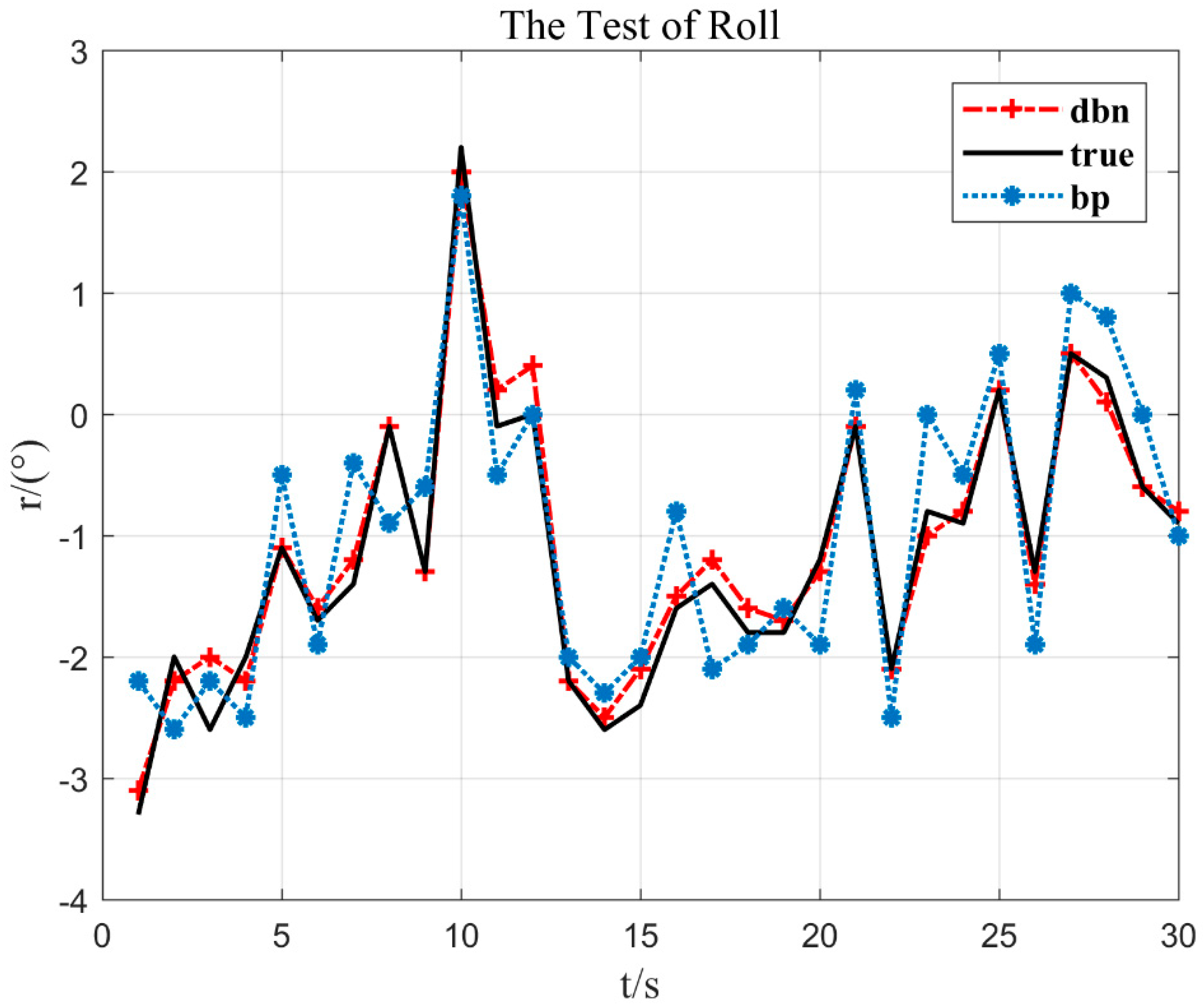
4.4. Experimental Results

After the training of the DBN model is completed, it can be used for online diagnosis of angle sensor faults. The following is a simulation verification of the pitch, roll, and yaw three sensor in the injection faults.

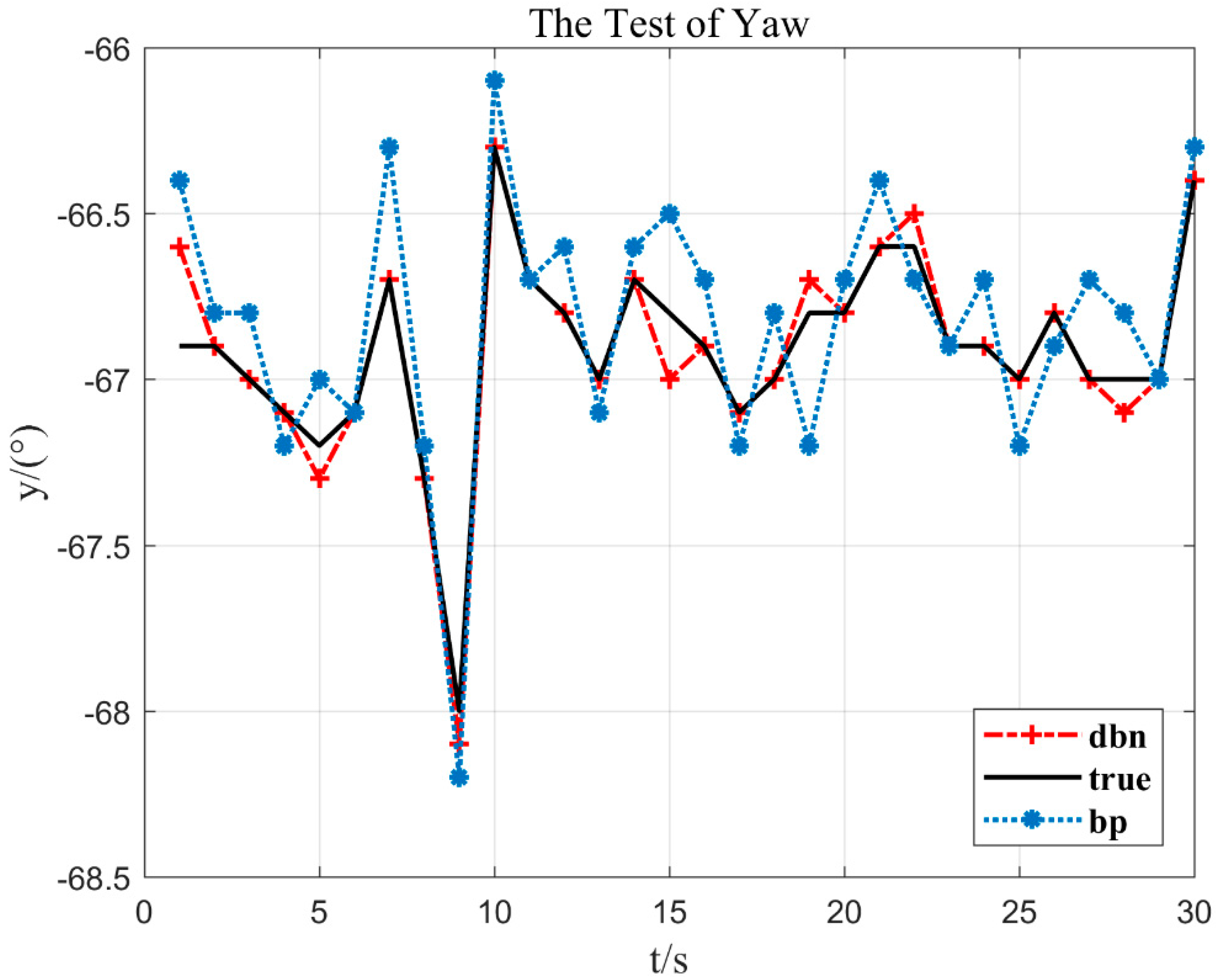
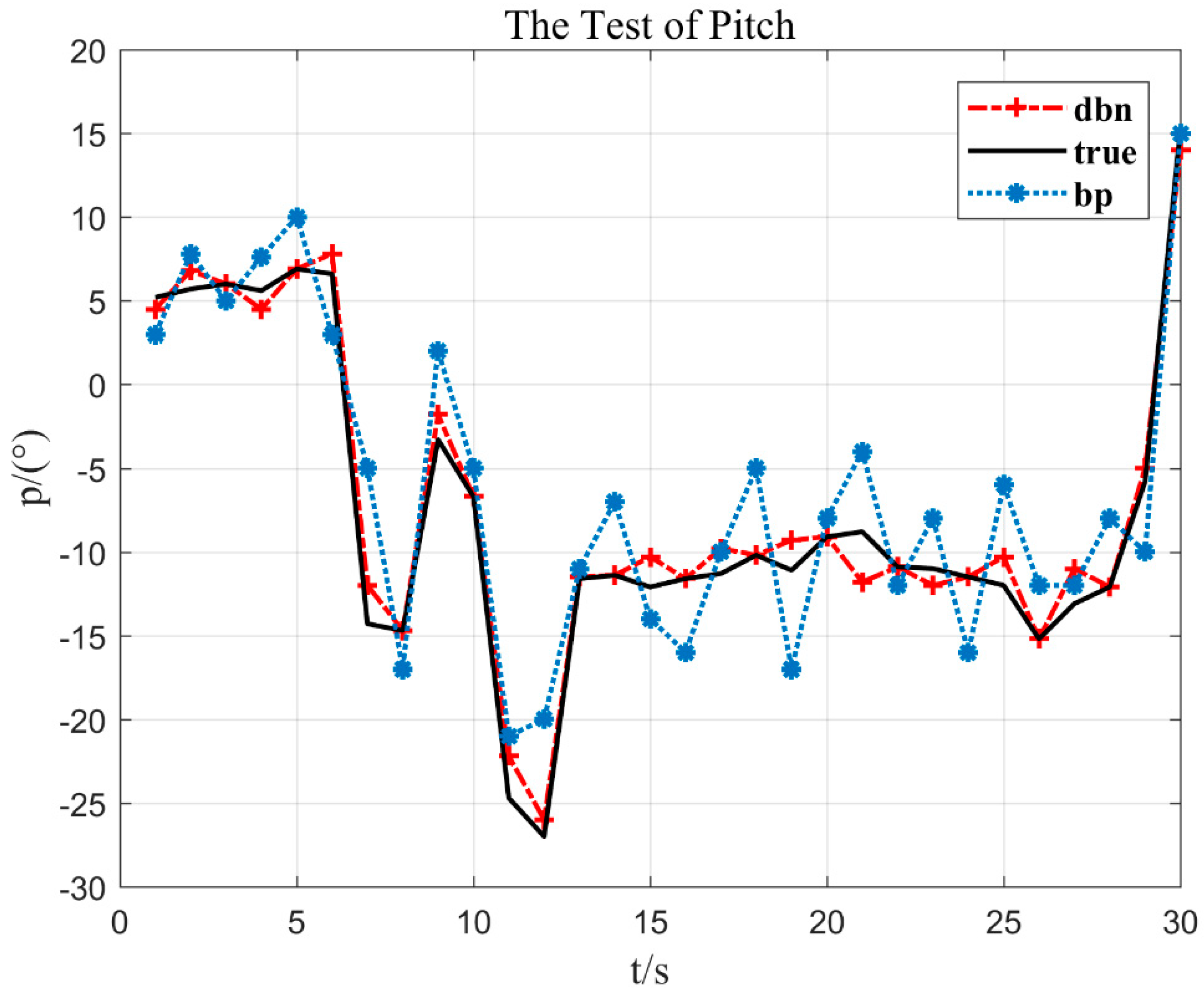
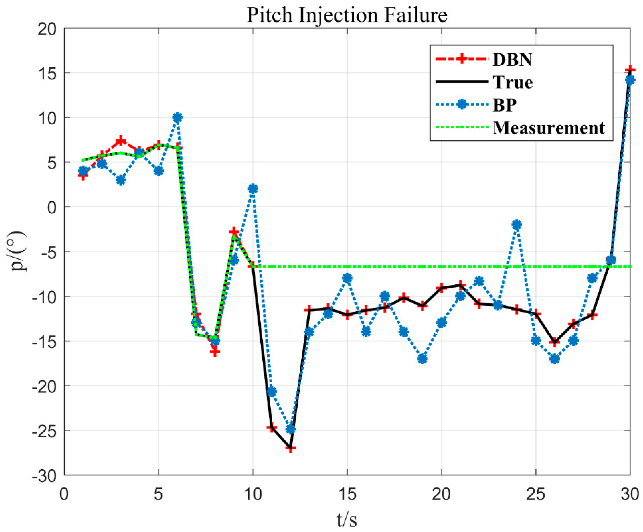
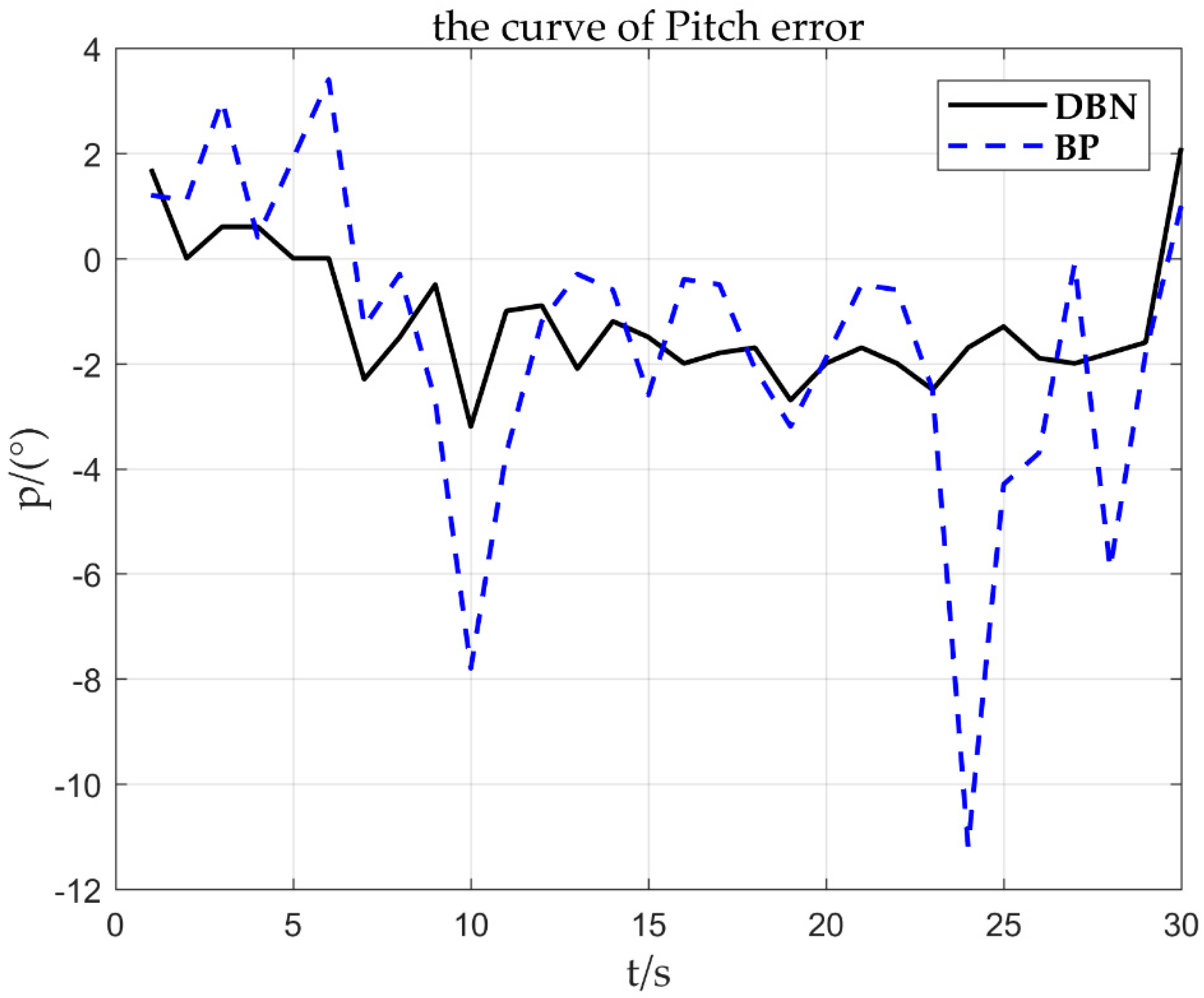
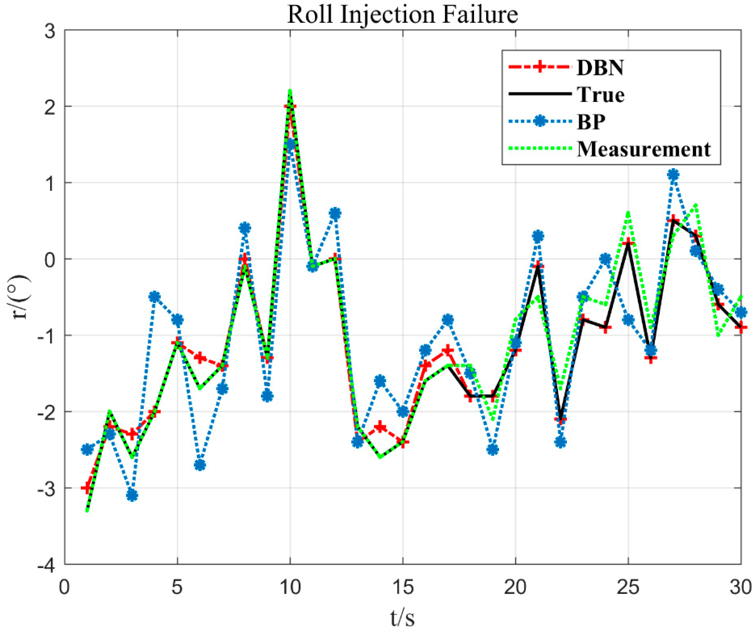
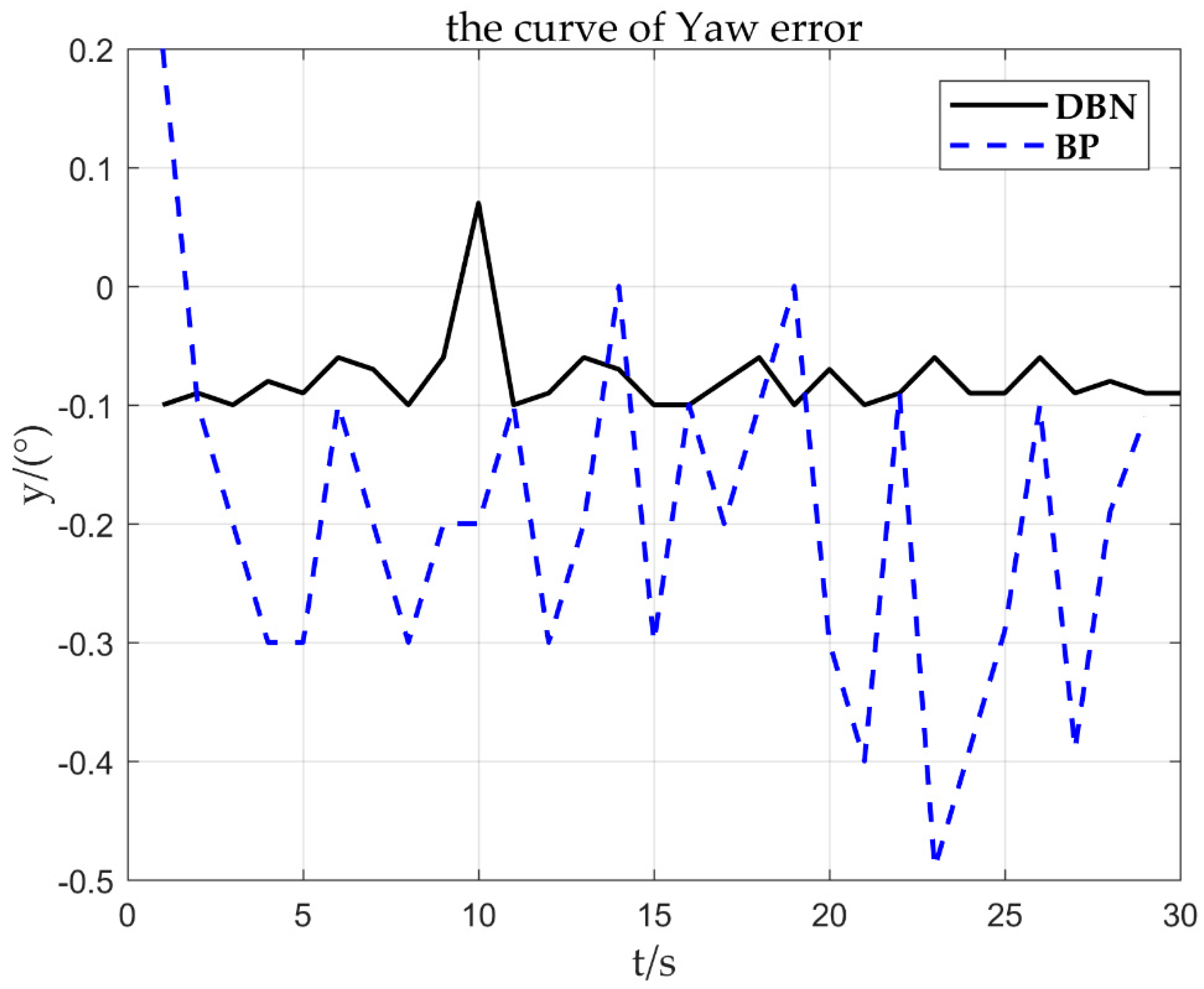
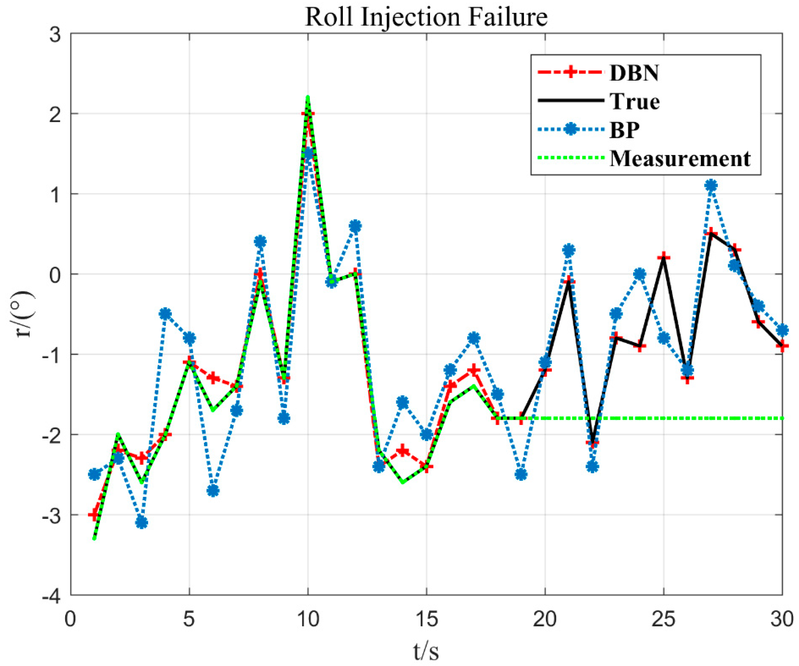
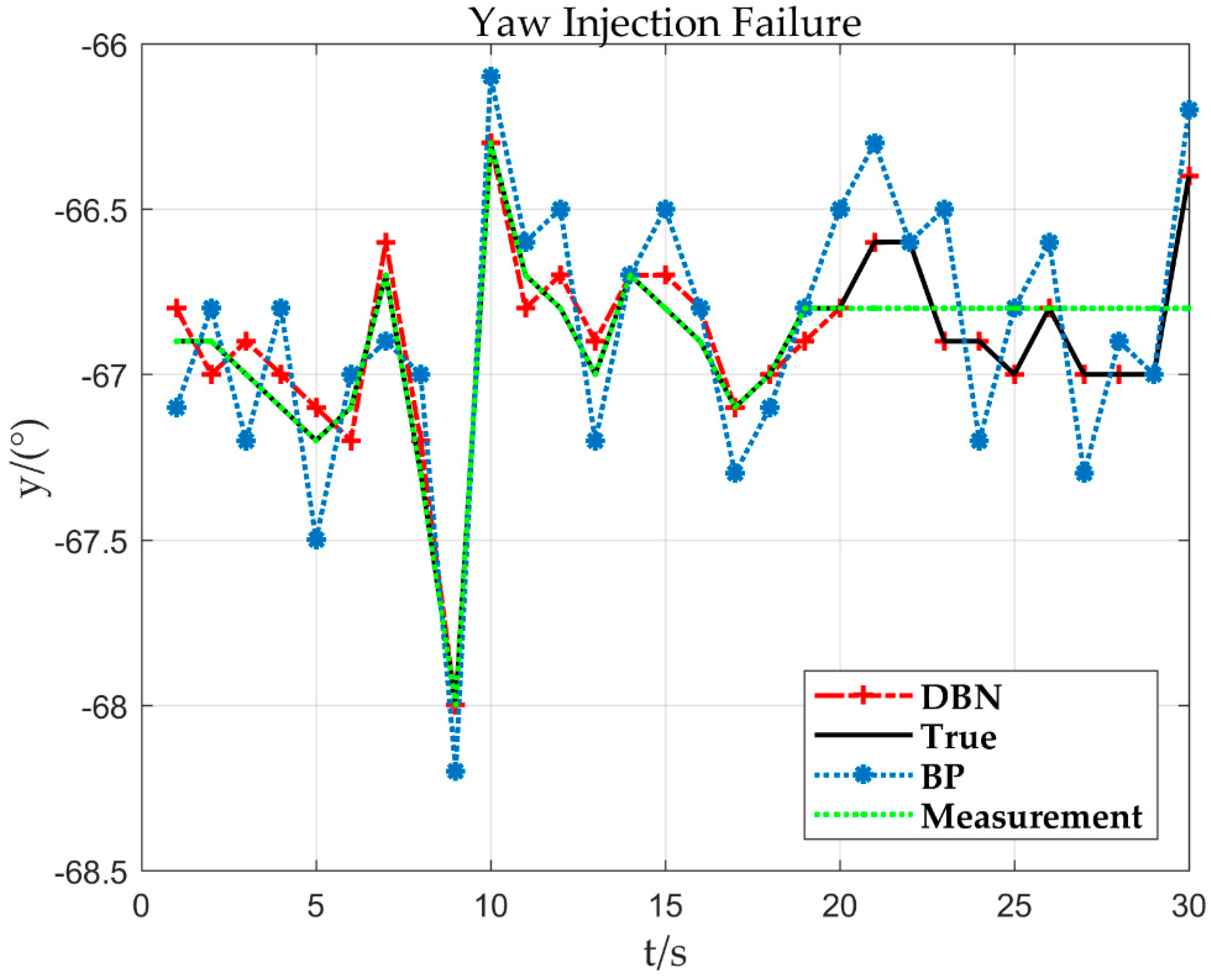
4.4.1. Sensor Stuck Fault Diagnosis

1. Pitch injection failure

In Figure 11, after the 10 s injection fault, the measurement value does not change any more. The method DBN proposed in the paper can fit the measured value more accurately. When the sensor fault is detected, the output value estimated by the DBN is used to replace the measurement value of the sensor, which provides a guarantee for the safe flight of the UAV.

2. Roll injection failure

In Figure 12, at 10 s of flight time (x = 10), the flying hand hits about 2% of the crossbar (y = 2.2°) to the right, and the duration of the entire crossbar is about 8 s to 10 s. Then, it leaned to the left again. Corresponding to the actual flight situation, the flying hand went to the right and rolled the bar, but it was released again. Therefore, the embodiment of the posture is to tilt to the right and immediately reverse the brake to slow down. According to this situation, the DBN model proposed in this paper can respond well to the stroke situation. When the sensor fault is detected, the output value estimated by the DBN is used to replace the measurement value of the sensor.

3. Yaw injection Failure

As can be seen in the trend of the curve in Figure 13, the aircraft yaw is −68° (y = −68°) at 9 s of flight time (x = 9). Nevertheless, at about 10 s, the yaw changes and the value increases from small to large, indicating that the aircraft has rotated clockwise. When the sensor fault is detected, the output value estimated by the DBN is used to replace the measurement value of the sensor.

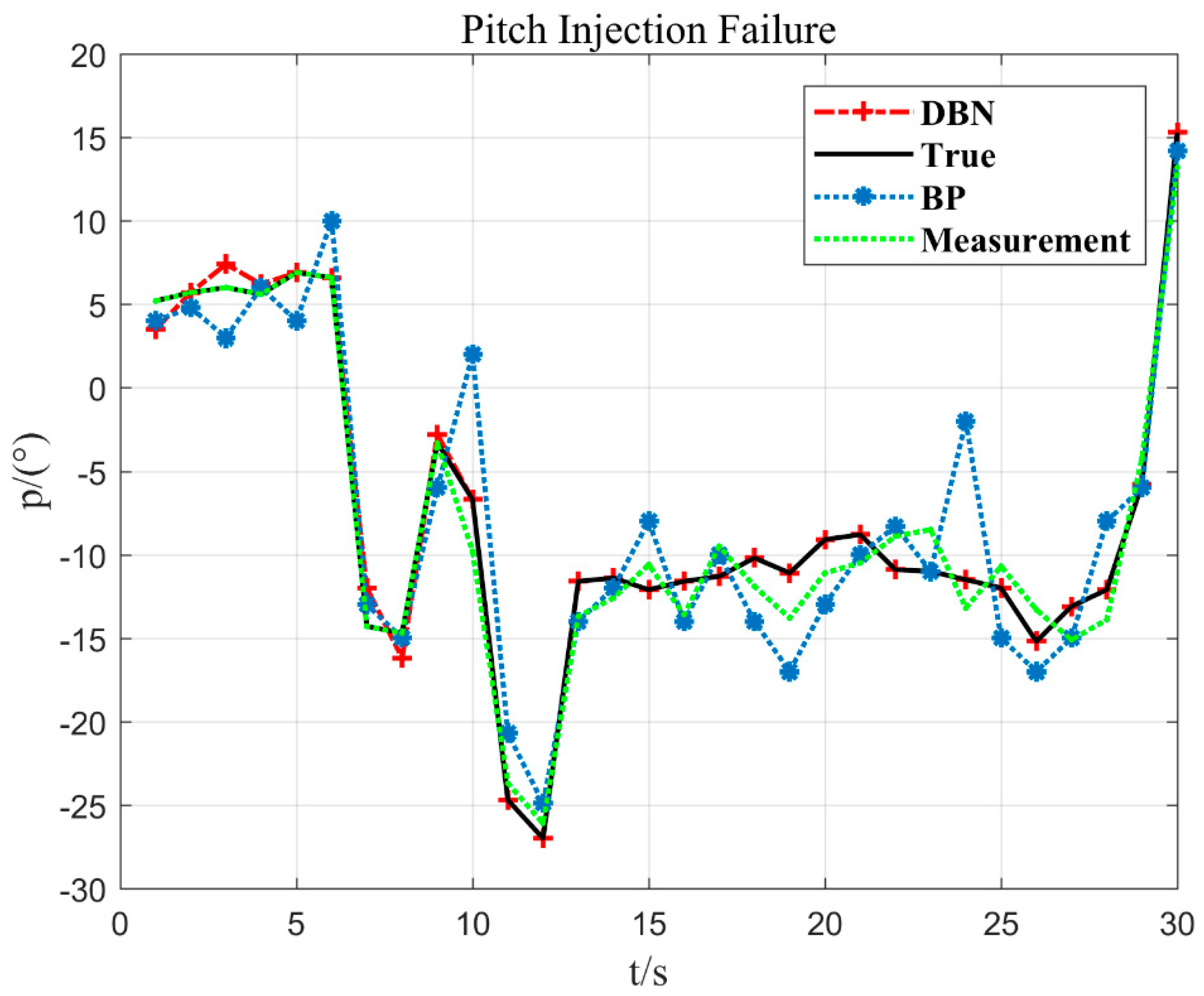
4.4.2. Sensor Constant Deviation Fault Diagnosis

1. Pitch injection failure

Taking the pitch sensor fault as an example, 2°/s constant deviation fault is injected at 10 s, and other simulation conditions are unchanged. The results are as follows.

As can be seen from Figure 15, the DBN network has a smaller and more accurate estimation error than the BP network. In order to further judge the type of fault, linearity fitting is used to obtain $\tilde{k}$ and $\tilde{a}$. The fault fitting result shown in Figure 14 is $\tilde{k}$ = 0.957, $\tilde{a}$ = 2.135, and the fault corresponding to the deviation is about 2. It can be obtained from Figure 15 that the $K_t$ is set to 1.8. By fitting the parameter $\tilde{a}$, it can be quickly inferred that the fault type is the sensor constant deviation fault. After the constant deviation fault is identified, the deviation of $\tilde{a}$ is corrected based on the sensor fault signal to achieve reconstruction of the fault signal.

2. Roll injection failure

Taking the roll sensor fault as an example, 0.3°/s constant deviation fault is injected at 18 s, and other simulation conditions are unchanged. The results are as follows.

From Figure 16, the fault fitting result is $\tilde{k}$ = 1.023, $\tilde{a}$ = 0.295, and the corresponding deviation is about 0.3. It can be obtained from Figure 17 that the $K_t$ is set to 0.3. By fitting the parameter $\tilde{a}$, it can be quickly inferred that the fault type is the sensor constant deviation fault. After the constant deviation fault is identified, the deviation of $\tilde{a}$ is corrected based on the sensor fault signal to achieve reconstruction of the fault signal.

3. Yaw injection failure

Taking the yaw sensor fault as an example, 0.08°/s constant deviation fault is injected at 21 s, and other simulation conditions are unchanged. The results are as follows.

The fault fitting result obtained by Figure 18 is $\tilde{k}$ = 0.975, $\tilde{a}$ = 0.078, and the corresponding deviation is about 0.08. It can be obtained from Figure 19 that the $K_t$ is set to 0.07. By fitting the parameter $\tilde{a}$, it can be quickly inferred that the fault type is the sensor constant deviation fault. After the constant deviation fault is identified, the deviation of $\tilde{a}$ is corrected based on the sensor fault signal to achieve reconstruction of the fault signal.

From all the above simulation figures, it can be concluded that compared with the traditional BP network model, the DBN network model proposed in the paper can more accurately estimate the UAV’s pitch, yaw, roll, and actively respond to the UAV’s stroke. Whether the sensor is faulty or not depends on whether the measured value is a fixed value at a certain time. When it comes to faults, fault isolation is immediately performed to ensure safe operation of the rotor UAV flight system.

5. Conclusions and Future Works

In the paper, the DBN method based on data-driven methods is applied to the fault diagnosis of the rotor UAV flight system sensors, which effectively solves the problems of the shallow neural networks, such as over-fitting, local minimum, generalization ability, complex functions, insufficient representation ability, and so on, by establishing a deep network structure. The simulation results show that compared with the BP model, the fault diagnosis model has higher convergence speed and diagnostic accuracy and can be extended to sensor diagnosis of other systems. The method currently realizes the real-time fault diagnosis and is applicable to complex the rotor UAV nonlinear systems. On the basis of this, the memory characteristics of long- short-term memory networks (LSTM) can be used to explore the short-term fault prediction of sensors, and to curb the working state of the sensor anytime and anywhere and enable the fault to be effectively prevented before it occurs, which is a necessary means to ensure safe and efficient operation of the rotor UAV. Therefore, the current state of the rotor UAV flight system sensor is estimated in terms of big data mining to realize the system’s conditional maintenance and avoid major safety accidents.

In a word, based on the research of the paper, it is indispensable to analyze the different models of different models of UAVs to verify the applicability of the model. In addition, in terms of improving system reliability, it is necessary to carry out deep excavation of the rotor UAV flight data in order to realize the conditional maintenance and life prediction of the equipment.

References

1. Huo, Y.; Dong, X.; Lu, T.; Xu, W.; Yuen, M. Distributed and Multilayer UAV Networks for Next-Generation Wireless Communication and Power Transfer: A Feasibility Study. IEEE Internet Things J. 2019, 6, 7103–7115. [Google Scholar] [CrossRef]
2. Gao, Y.H.; Zhao, D.; Li, Y.B. UAV Sensor Fault Diagnosis Technology: A Survey. Appl. Mech. Mater. 2012, 220, 1833–1837. [Google Scholar] [CrossRef]
3. Ducard, G.; Rudin, K.; Omari, S.; Siegwart, R. Strategies for Sensor-fault Compensation on UAVs: Review, Discussions & Additions. In Proceedings of the 2014 European Control Conference (ECC), Strasbourg, France, 24–27 June 2014. [Google Scholar]
4. Hansen, S.; Blanke, M. Diagnosis of Airspeed Measurement Faults for Unmanned Aerial Vehicles. IEEE Trans. Aerosp. Electron. Syst. 2014, 50, 224–239. [Google Scholar] [CrossRef]
5. López-Estrada, F.R.; Ponsart, J.C.; Theilliol, D.; Astorga-Zaragoza, C.M.; Zhang, Y.M. Robust Sensor Fault Diagnosis and Tracking Controller for a UAV Modelled as LPV System. In Proceedings of the International Conference on Unmanned Aircraft Systems (ICUAS), Orlando, FL, USA, 27–30 May 2014. [Google Scholar]
6. Ding, S.X. Model-Based Fault Diagnosis Techniques. IFAC Pap. 2016, 49, 50–56. [Google Scholar]
7. Yoon, S.; Kim, S.; Bae, J.; Kim, Y.; Kim, E. Experimental evaluation of fault diagnosis in a skew-configured UAV sensor system. Control Eng. Pract. 2011, 19, 158–173. [Google Scholar] [CrossRef]
8. Freeman, P.; Seiler, P.; Balas, G.J. Air data system fault modeling and detection. Control Eng. Pract. 2013, 21, 1290–1301. [Google Scholar] [CrossRef]
9. Remus, A. Fault Diagnosis and Fault-Tolerant Control of Quadrotor UAVs. Ph.D. Thesis, Wright State University, Dayton, OH, USA, 2016. [Google Scholar]
10. Yu, P.; Liu, D. Data-driven prognostics and health management: A review of recent advances. Chin. J. Sci. Instrum. 2014, 35, 481–495. [Google Scholar]
11. Kim, J.H. Time Frequency Image and Artificial Neural Network Based Classification of Impact Noise for Machine Fault Diagnosis. Int. J. Precis. Eng. Manuf. 2018, 19, 821–827. [Google Scholar] [CrossRef]
12. Guo, D.; Zhong, M.; Ji, H.; Liu, Y.; Yang, R. A hybrid feature model and deep learning based fault diagnosis for unmanned aerial vehicle sensors. Neurocomputing 2018, 319, 155–163. [Google Scholar] [CrossRef]
13. Younes, Y.A.; Rabhi, A.; Noura, H.; Hajjaji, A.E. Sensor fault diagnosis and fault tolerant control using intelligent-output-estimator applied on quadrotor UAV. In Proceedings of the International Conference on Unmanned Aircraft Systems (ICUAS), Arlington, VA, USA, 7–10 June 2016. [Google Scholar]
14. Sun, R.; Cheng, Q.; Wang, G.; Ochieng, W. A Novel Online Data-Driven Algorithm for Detecting UAV Navigation Sensor Faults. Sensors 2017, 17, 2243. [Google Scholar] [CrossRef] [PubMed]
15. Qi, J.; Zhao, X.; Jiang, Z.; Han, J. An Adaptive Threshold Neural-Network Scheme for Rotorcraft UAV Sensor Failure Diagnosis; Springer: Berlin/Heidelberg, Germany, 2007. [Google Scholar]
16. Shen, Y.; Wu, C.; Liu, C.; Wu, Y.; Xiong, N. Oriented Feature Selection SVM Applied to Cancer Prediction in Precision Medicine. IEEE Access 2018, 6, 48510–48521. [Google Scholar] [CrossRef]
17. Guo, Y.; Shuang, W.; Gao, C.; Shi, D.; Zhang, D.; Hou, B. Wishart RBM based DBN for polarimetric synthetic radar data classification. In Proceedings of the 2015 IEEE International Geoscience and Remote Sensing Symposium (IGARSS), Milan, Italy, 26–31 July 2015. [Google Scholar]
18. Senkul, F.; Altug, E. Adaptive control of a tilt—Roll rotor quadrotor UAV. In Proceedings of the 2014 International Conference on Unmanned Aircraft Systems (ICUAS), Orlando, FL, USA, 27–30 May 2014. [Google Scholar]
19. Zeng, Y.; Xu, J.; Zhang, R. Energy Minimization for Wireless Communication With Rotary-Wing UAV. IEEE Trans. Wirel. Commun. 2019, 18, 2329–2345. [Google Scholar] [CrossRef]
20. Mateo, G.; Luka, J. Gimbal Influence on the Stability of Exterior Orientation Parameters of UAV Acquired Images. Sensors 2017, 17, 401. [Google Scholar]
21. Warsi, F.A.; Hazry, D.; Ahmed, S.F.; Joyo, M.K.; Tanveer, M.H.; Kamarudin, H.; Razlan, Z.M. Yaw, Pitch and Roll controller design for fixed-wing UAV under uncertainty and perturbed condition. In Proceedings of the 2014 IEEE 10th International Colloquium on Signal Processing and its Applications, Kuala Lumpur, Malaysia, 7–9 March 2014. [Google Scholar]
22. Chao, Y.; Wu, J.; Wang, X. Roll and yaw control of unmanned helicopter based on adaptive neural networks. In Proceedings of the 2008 27th Chinese Control Conference, Kunming, China, 16–18 July 2008. [Google Scholar]
23. Altan, A.; Hacioglu, R. Modeling of three-axis gimbal system on unmanned air vehicle (UAV) under external disturbances. In Proceedings of the 2017 25th Signal Processing and Communications Applications Conference (SIU), Antalya, Turkey, 15–18 May 2017. [Google Scholar]
24. Rajesh, R.J.; Ananda, C.M. PSO tuned PID controller for controlling camera position in UAV using 2-axis gimbal. In Proceedings of the 2015 International Conference on Power and Advanced Control Engineering (ICPACE), Bangalore, India, 12–14 August 2015. [Google Scholar]
25. Jie, K.; Li, Z.; Zhong, W. Design of Robust Roll Angle Control System of Unmanned Aerial Vehicles Based on Atmospheric Turbulence Attenuation. In Proceedings of the 2010 8th World Congress on Intelligent Control and Automation, Jinan, China, 7–9 July 2010. [Google Scholar]
26. Wu, C.; Luo, C.; Xiong, N.; Zhang, W.; Kim, T. A Greedy Deep Learning Method for Medical Disease Analysis. IEEE Access 2018, 6, 20021–20030. [Google Scholar] [CrossRef]
27. Nasersharif, B. Noise Adaptive Deep Belief Network For Robust Speech Features Extraction. In Proceedings of the 2017 Iranian Conference on Electrical Engineering (ICEE), Tehran, Iran, 2–4 May 2017. [Google Scholar]
28. Chen, D.; Jiang, D.; Ravyse, I.; Sahli, H. Audio-Visual Emotion Recognition Based on a DBN Model with Constrained Asynchrony. In Proceedings of the 2009 Fifth International Conference on Image and Graphics, Xi’an, China, 20–23 September 2009. [Google Scholar]
29. Alkhateeb, J.H.; Alseid, M. DBN—Based learning for Arabic handwritten digit recognition using DCT features. In Proceedings of the 2014 6th International Conference on Computer Science and Information Technology (CSIT), Amman, Jordan, 26–27 March 2014. [Google Scholar]
30. Ke, W.; Chunxue, W.; Wu, Y.; Xiong, N. A New Filter Feature Selection Based on Criteria Fusion for Gene Microarray Data. IEEE Access 2018, 6, 61065–61076. [Google Scholar] [CrossRef]
31. Hajinoroozi, M.; Jung, T.P.; Lin, C.T.; Huang, Y. Feature extraction with deep belief networks for driver’s cognitive states prediction from eeg data. In Proceedings of the IEEE China Summit & International Conference on Signal & Information Processing (ChinaSIP), Chengdu, China, 12–15 July 2015. [Google Scholar]
32. Lei, Y.; Feng, J.; Jing, L.; Xing, S.; Ding, S. An intelligent fault diagnosis method using unsupervised feature learning towards mechanical big data. IEEE Trans. Ind. Electron. 2016, 63, 3137–3147. [Google Scholar]
33. Lin, B.; Guo, W.; Xiong, N.; Chen, G.; Vasilakos, A.V.; Zhang, H. A Pretreatment Workflow Scheduling Approach for Big Data Applications in Multicloud Environments. IEEE Trans. Netw. Serv. Manag. 2016, 13, 581–594. [Google Scholar] [CrossRef]
34. Liu, X.; Hu, Y.; Xu, Z.; Ren, Y.; Gao, T. Fault diagnosis for hydraulic system of naval gun based on BP-Adaboost model. In Proceedings of the 2017 Second International Conference on Reliability Systems Engineering (ICRSE), Beijing, China, 10–12 July 2017; pp. 1–6. [Google Scholar]
Figure 1. Rotor unmanned aerial vehicle (UAV) physical axis in (a) the axis of X, Y, (b) the axis of Z, and (c) the definition of Axis direction.
Electronics 08 01350 g001aElectronics 08 01350 g001b
Figure 2. Deep belief network (DBN) basic network structure.
Electronics 08 01350 g002
Figure 3. DBN feature extraction process in (a)the restricted Boltzmann machines (RBM) of the first layer, (b) the RBM of the second layer, and (c) the RBM of the third layer.
Electronics 08 01350 g003
Figure 4. Fault diagnosis algorithm flow.
Electronics 08 01350 g004
Figure 5. Accuracy of different RBM layers and training samples.
Electronics 08 01350 g005
Figure 6. The relationship between the number of iteration times and the error.
Electronics 08 01350 g006
Figure 7. Effect of RBM layer number on classification accuracy.
Electronics 08 01350 g007
Figure 8. The test of roll.
Electronics 08 01350 g008
Figure 9. The test of yaw.
Electronics 08 01350 g009
Figure 10. The test of pitch.
Electronics 08 01350 g010
Figure 11. Pitch 10 s and −6.7° injection failure.
Electronics 08 01350 g011
Figure 12. Roll 18 s and −1.8° injection failure.
Electronics 08 01350 g012
Figure 13. Yaw 21 s and −66.6° injection failure.
Electronics 08 01350 g013
Figure 14. Sensor deviation 2°/s pitch response curve.
Electronics 08 01350 g014
Figure 15. 2°/s error curve.
Electronics 08 01350 g015
Figure 16. Sensor deviation 0.3°/s roll response curve.
Electronics 08 01350 g016
Figure 17. 0.3°/s error curve.
Electronics 08 01350 g017
Figure 18. Sensor deviation 0.08°/s yaw response curve.
Electronics 08 01350 g018
Figure 19. 0.08°/s error curve.
Electronics 08 01350 g019