Support Vector Regression for the Modeling and Synthesis of Near-Field Focused Antenna Arrays

Abstract

The powerful support vector regression framework is proposed in a novel method for near-field focusing using antenna arrays. By using this machine-learning method, the set of weights required in the elements of an array can be calculated to achieve an assigned near-field distribution focused on one or more positions. The computational cost is concentrated in an initial training process so that the trained system is fast enough for applications where moving devices are involved. The increased learning capabilities of support vector machines allow using a reduced number of training samples. Thus, these training samples may be generated with a prototype or a convenient electromagnetic analysis tool, and hence realistic effects, such as coupling or the individual radiation patterns of the elements of the arrays, are accounted for. Illustrative examples are presented.

1. Introduction

Near-field focusing (NFF) [1,2,3,4,5] is one of the state-of-the-art topics related to antenna design that is gaining more attention in the recent years. It has become one of the most interesting approaches to emerging applications such as RFID [2,4], medical hyperthermia [6], wireless energy transfer (WET) [7], wireless energy and information transfer (WEIT) [8,9], imaging, Internet of things (IoT) or 5G mobile telephony, which are based on wireless links between devices usually located at short distances. NFF allows antenna arrays to concentrate the energy on an assigned position or spot in the near-field (NF) region of the antenna, reducing the waste of energy directed to positions of space where it is not necessary. The conjugate-phase (CP) method proposed in [2,10,11] is an excellent technique for calculating the phase-shift that must be applied to each array element so that all the signal contributions from the individual elements arrive in-phase to the position of interest, creating a constructive interference that increases the field level at such position. This is a robust and simple approach whose performance has been undoubtedly proven. However, the CP method has been lacking for certain cases where it is limited, for example in emerging applications with more demanding specifications that require concentrating the field on more than one focal point or arbitrary volumes. In such cases, near-field multi-focusing (NFMF) has arisen as an excellent alternative [12,13].

NFMF is based on the minimization of a proper cost function designed to account for all the requirements. Different optimization techniques are used to calculate the set of weights that must be applied to the array elements so that the resulting field distribution is focused on the assigned spots. Although the resulting method is flexible and powerful with increased focusing performance, it is time consuming due to the iterative nature of the optimization techniques involved. In the case of applications requiring fast adaptation, for example because moving devices are involved, this could represent an important limitation as the time required to calculate the new weights to focus on the new positions could be unacceptable.

Recently, in [14] neural networks (NN) [15] have been proposed as an alternative to optimization for NFMF applications, adapting previous successful approaches used for far field (FF) synthesis problems [16,17]. The resulting focusing performance is similar to that achieved using optimization techniques, but its time–cost is strongly reduced once the NN has been trained; it is able to calculate the weights required to achieve a given field distribution without relevant delay. All the computing time is concentrated in the previous training step, but providing solutions almost in real time once trained. The training or learning of any machine learning (ML) system consists of presenting known pairs of inputs and outputs so that the system is able to extract the relationship between them and provide outputs to new inputs. In [14], the training pairs presented to the NN are samples of the NF distributions and the weights applied to the array to achieve them. Although NNs are a very popular tool in the framework of ML methods, other alternatives have been shown to present improved learning capabilities, avoiding the problem of overfitting [15] if the NN is trained excessively, and requiring much less training data. In [14], the number of pairs required to train the NN is in the order of 5000. If the training patterns are obtained through simulation, the time requested to obtain such a number of patterns might be excessive; obtaining them through measurement of a real antenna is impossible in practice. In this paper we propose the use of support vector regression (SVR), a powerful ML method based on support vector machines (SVM) and the associated structural risk minimization principle (SRM) [18] to obtain the weights to be applied to the array elements so that an antenna array is able to multifocus or to generate a near-field (NF) distribution complying with the specifications. It requires a strongly reduced set of training patterns with respect to NNs, so that obtaining them becomes easier, and the system still operates fast enough for real time applications. Although SVR has been used in [19] for NFF applications, it was only used as an auxiliary tool used to calculate a coupling matrix required to model interaction between elements in the results of a conventional optimization method. In this paper we propose using SVR directly to synthesize the weights required for focusing on some assigned points.

This paper is organized as follows: Section 2 presents the use of SVR to create a model of the array able to relate field samples and weights. In Section 3 this model is used to perform the synthesis. Some illustrative results are presented in Section 4. These results and some conclusions are discussed in Section 5.

2. Support Vector Regression-Based Inverse Model of the Array

The field radiated at a certain position $\overrightarrow{r}$ by an antenna array with N elements is given by the superposition of the field radiated by its individual elements. A general and simple formulation representing this sum of contributions is

$$E\left(\overrightarrow{r}\right)=\sum _{n=1}^N{\omega }_n·g_n\left(\overrightarrow{r}\right)={\mathbf{g}}^T\left(\overrightarrow{r}\right)·\mathbf{w}$$

(1)

where $E\left(\overrightarrow{r}\right)$ is the value of the considered component of the field at $\overrightarrow{r}$, ${\omega }_n$ is the feeding weight applied to the n-th array element, whose contribution to the field at $\overrightarrow{r}$ is $g_n\left(\overrightarrow{r}\right)$. These values are also represented in vector form as $\mathbf{w}={[{\omega }_1,{\omega }_2,\dots ,{\omega }_N]}^T$ and $\mathbf{g}\left(\overrightarrow{r}\right)={[g_1\left(\overrightarrow{r}\right),g_2\left(\overrightarrow{r}\right),\dots ,g_N\left(\overrightarrow{r}\right)]}^T$, with ${(.)}^T$ representing the transpose operator.

If M positions of the near-field region of the antenna are evaluated, ${\overrightarrow{r}}_m,m=1\dots M$, Equation (1) may be rewritten in matrix form as

$$\mathbf{e}=\mathbf{G}·\mathbf{w}$$

(2)

with $\mathbf{e}={[E\left({\overrightarrow{r}}_1\right),E\left({\overrightarrow{r}}_2\right),\dots ,E\left({\overrightarrow{r}}_M\right)]}^T$ and $\mathbf{G}={[\mathbf{g}\left({\overrightarrow{r}}_1\right),\mathbf{g}\left({\overrightarrow{r}}_2\right),\dots ,\mathbf{g}\left({\overrightarrow{r}}_M\right)]}^T$. A proper modeling of the array involves determining or calculating $\mathbf{G}$. However, for synthesis purposes an inverse model is more adequate.

In the usual case of $M>N$ (i.e., the number of positions where the field is evaluated is greater than the number of elements in the array) Equation (2) represents an overdetermined system of linear equations. If a least-squares criterion is chosen to find a solution, the problem becomes

$$\underset{\mathbf{w}}{minimize}\left|\right|\mathbf{e}-\mathbf{G}·{\mathbf{w}\left|\right|}^2$$

(3)

where $\left|\right|.\left|\right|$ stands for the Euclidean norm.

The solution to Equation (3) is well known [20] and given by

$$\mathbf{w}={({\mathbf{G}}^H·\mathbf{G})}^{-1}·{\mathbf{G}}^H·\mathbf{e}={\mathbf{G}}^{+}·\mathbf{e}$$

(4)

where ${\mathbf{G}}^{+}$ is the pseudoinverse matrix for the overdetermined problem, and it represents an inverse model of the antenna array. Equation (4) shows that a linear model $\mathbf{A}={\mathbf{G}}^{+}$ may be obtained to calculate the weights that must be applied to an antenna array so that it radiates according to a given field distribution specified by its samples, $\mathbf{w}=\mathbf{A}·\mathbf{e}$.

The SVR framework is proposed to calculate the mentioned model. Let us consider that a set of P pairs $\{{\mathbf{w}}^{\left(p\right)},{\mathbf{e}}^{\left(p\right)}\},p=1\dots P$, are available for training purposes. Each training pair (or training pattern) consists of a vector of weights applied to the elements of the array and the corresponding field distribution represented by its samples. In this training dataset, the inputs correspond to the field distributions represented by their samples, so that the number of samples for each pattern is defined by the number M of locations in the NF region of the antenna that are considered. The outputs are represented by the complex weights applied to the elements of the array, i.e., a total of N complex values for each sample. It is straightforward that the total number of values involved is $M·P$ in the inputs and $N·P$ in the outputs. These training patterns may have been obtained by measurements, EM simulations or by any means. If they are obtained using a method that accounts for the realistic properties of the array (including coupling effects between elements, non-idealities, etc.), the training patterns also take these properties into account, hence increasing its accuracy.

If we focus on the n-th element of the array in order to obtain the feeding weight that must be applied to it, the SRM principle establishes that the n-th row of $\mathbf{A}$, ${\mathbf{a}}_n$, can be obtained through minimizing a cost function given by [18]:

$$J\left({\mathbf{a}}_n\right)=\frac{1}{2}\left|\right|{\mathbf{a}}_n{\left|\right|}^2+C\sum _{p=1}^P{|{\omega }_n^{\left(p\right)}-{\mathbf{a}}_n·{\mathbf{e}}^{\left(p\right)}|}_{\epsilon }$$

(5)

where

$$|{\omega }_n^{\left(p\right)}-{\mathbf{a}}_n·{\mathbf{e}}^{\left(p\right)}{|}_{\epsilon }=\max (0,|{\omega }_n^{\left(p\right)}-{\mathbf{a}}_n·{\mathbf{e}}^{\left(p\right)}|-\epsilon )$$

(6)

is Vapnik’s $\epsilon$-insensitive loss function, and $C>0$ is a penalty value used to balance the model complexity (controlled by the first term of Equation (5)) and the cost of deviations larger than $\epsilon$. This parameter is related to the precision of the field sampling, the noise or any other uncertainty factor that might affect the accuracy of the training patterns. This cost function implies the choice of a linear kernel for the SVR [18]. This is a straightforward choice due to the linear relation between inputs and outputs made explicit in Equation (4).

In order to solve this minimization problem, a set of positive slack variables ${\xi }_p$ and ${\tilde{\xi }}_p$ are introduced so that Equation (5) may be rewritten as a constrained minimization problem given by

$$\underset{{\mathbf{a}}_n}{minimize}\frac{1}{2}\left|\right|{\mathbf{a}}_n{\left|\right|}^2+C\sum _{p=1}^P({\xi }_p+{\tilde{\xi }}_p)$$

(7)

subject to

$$\begin{array}{c}\hfill {\mathbf{a}}_n·{\mathbf{e}}^{\left(p\right)}-{\omega }_n^{\left(p\right)}\le \epsilon +{\xi }_p,\forall p=1\dots P\\ \hfill {\omega }_n^{\left(p\right)}-{\mathbf{a}}_n·{\mathbf{e}}^{\left(p\right)}\le \epsilon +{\tilde{\xi }}_p,\forall p=1\dots P\\ \hfill {\xi }_p,{\tilde{\xi }}_p\ge 0,\forall p=1\dots P\end{array}$$

This problem is usually solved making use of the Lagrange multiplier technique [18], which leads to an optimal regressor (i.e., the optimal values of the n-th row of model $\mathbf{A}$) given by the following expression:

$${\widehat{\mathbf{a}}}_n=\sum _{p=1}^P({\tilde{\alpha }}_p-{\alpha }_p){\mathbf{e}}^{\left(p\right)}$$

(8)

which is a function of the field distribution training patterns, linearly combined using ${\tilde{\alpha }}_p$ and ${\alpha }_p$, positive Lagrange multipliers resulting from the maximization of the quadratic dual problem expressed as

$$W(\tilde{\alpha },\alpha )=-\sum _{p=1}^P\epsilon ({\tilde{\alpha }}_p+{\alpha }_p)+\sum _{p=1}^P{\omega }_n^{\left(p\right)}({\tilde{\alpha }}_p+{\alpha }_p)-\frac{1}{2}\sum _{p,q=1}^P({\tilde{\alpha }}_p+{\alpha }_p)({\tilde{\alpha }}_q+{\alpha }_q)\langle {\mathbf{e}}^{\left(p\right)},{\mathbf{e}}^{\left(q\right)}\rangle$$

(9)

subject to $0\le \tilde{\alpha },\alpha \le C$. The expression $\langle {\mathbf{e}}^{\left(p\right)},{\mathbf{e}}^{\left(q\right)}\rangle$ stands for the inner product, and it is applied to pairs of near-field distributions taken from the training patterns. The solution of this dual quadratic programming (QP) problem can be efficiently found taking advantage of its convexity (for example, using [21,22]). The support vector theory states that only some training patterns (typically less than P) contribute to Equation (8) while the other terms in the summation are canceled because their corresponding Lagrange multipliers are both zero-valued. The training patterns with non-null multipliers are referred to as support vectors.

The solution to Equation (8) allows calculating the weight ${\omega }_n$ that must be applied to the n-th element of the array. This regression must be repeated for the total N elements, obtaining the rows of the estimated model $\widehat{\mathbf{A}}$. Finally, the total set of weights to be applied to the array elements to produce a given field distribution can be estimated as

$$\widehat{\mathbf{w}}=\widehat{\mathbf{A}}·\mathbf{e}.$$

(10)

The number of training patterns P used to perform the regression is a critical choice for the accuracy of the model in ML methods. Unfortunately, none of the methods proposed in the literature for the choice of P has been accepted as valid in general situations. A strategy based on the cross-evaluation of an independent test or validation set (usually a subset of the available patterns not used for training) is typically followed. In the examples presented along this paper, the validation set consists of new patterns obtained using the same procedure as with the training set. In all cases, the number of validation patterns has been chosen to be $10\%$ of the training set, i.e., $0.1P$. Although other machine learning methods may be affected by the problem of overfitting (for example neural networks [15]), the SRM principle applied in SVR guarantees robustness against overfitting if P is too high, and improved learning capabilities (i.e., a smaller P is necessary for similar performance).

Handling Complex Values in Real-Valued Schemes

The optimization problems proposed in Equations (7) and (9) are complex-valued, as both the field samples and the weights applied to the array are complex, and also the model relating them is composed of complex values. Nowadays most optimization schemes and toolboxes are able to handle complex values, but some ML methods are designed to work with real numbers. In such cases, the regression can be reformulated to be handled by the real-valued algorithms.

Let us consider a vector of real values $\tilde{\mathbf{w}}={[\Re \left\{{\mathbf{w}}^T\right\}\Im \left\{{\mathbf{w}}^T\right\}]}^T$ obtained by stacking the real and imaginary parts of the weight vector $\mathbf{w}$. The real and imaginary parts of the samples of the field distribution may also be stacked to create an extended real-valued vector $\tilde{\mathbf{e}}={[\Re \left\{{\mathbf{e}}^T\right\}\Im \left\{{\mathbf{e}}^T\right\}]}^T$ so that both extended vectors are related according to

$$\tilde{\mathbf{w}}=\tilde{\mathbf{A}}·\tilde{\mathbf{e}}$$

(11)

with an extended model relating both vectors given by

$$\tilde{\mathbf{A}}=\left[\begin{array}{cc}\hfill \Re \left\{\mathbf{A}\right\}& -\Im \left\{\mathbf{A}\right\}\\ \hfill \Im \left\{\mathbf{A}\right\}& \Re \left\{\mathbf{A}\right\}\end{array}\right].$$

(12)

The optimization problem Equation (7) can be adapted to deal with this extended model by simply considering this real-valued formulation. The regression must be applied $2N$ times to calculate the rows of the extended model $\tilde{\mathbf{A}}$:

$$\underset{{\mathbf{a}}_{n^{\prime }}}{minimize}\frac{1}{2}\left|\right|{\mathbf{a}}_{n^{\prime }}{\left|\right|}^2+C\sum _{p=1}^P({\xi }_p+{\tilde{\xi }}_p),\mathrm{for}{n}^{\prime }=1\dots 2N$$

(13)

subject to

$$\begin{array}{c}\hfill {\mathbf{a}}_{n^{\prime }}·{\mathbf{e}}^{\left(p\right)}-{\omega }_{n^{\prime }}^{\left(p\right)}\le \epsilon +{\xi }_p,\forall p=1\dots P\\ \hfill {\omega }_{n^{\prime }}^{\left(p\right)}-{\mathbf{a}}_{n^{\prime }}·{\mathbf{e}}^{\left(p\right)}\le \epsilon +{\tilde{\xi }}_p,\forall p=1\dots P\\ \hfill {\xi }_p,{\tilde{\xi }}_p\ge 0,\forall p=1\dots P.\end{array}$$

From the extended model it is straightforward to calculate the complex-valued model.

It is interesting to notice that the training dataset has to be modified to use this real-valued approach. In this case, instead of using the weight vector and the complex samples of the corresponding field distribution, the real-valued version must also be used by stacking the real and imaginary parts of both vectors, $\{{\tilde{\mathbf{w}}}^{\left(p\right)},{\tilde{\mathbf{e}}}^{\left(p\right)}\},p=1\dots P$, with ${\tilde{\mathbf{w}}}^{\left(p\right)}={[\Re \left\{{\mathbf{w}}^{\left(p\right)T}\right\}\Im \left\{{\mathbf{w}}^{\left(p\right)T}\right\}]}^T$ and ${\tilde{\mathbf{e}}}^{\left(p\right)}={[\Re \left\{{\mathbf{e}}^{\left(p\right)T}\right\}\Im \left\{{\mathbf{e}}^{\left(p\right)T}\right\}]}^T$. In this training dataset, the inputs correspond again to the field distributions represented by their samples, but the number of values for each pattern is $2M$ due to the separation of real and imaginary parts. In the same way, the outputs are represented by $2N$ real values for each sample. The total number of values involved is now $2M·P$ in the inputs and $2N·P$ in the outputs.

3. Near-Field Focusing Using the SVR-Based Inverse Model

Some previous methods proposed for near-field focusing aplications are based on the use of models relating a target NF distribution and the weights applied to the array elements. For example, the method presented in [13] makes use of a typical formulation based on a near-field array factor represented in matrix form. In order to specify the NF requirements it builds a target field distribution defined as a unitary value for the samples corresponding to the focal points and null values at any other position. The same procedure for the specification of the NF was used in the NN method proposed in [14]. It is a very flexible specification procedure as far as it allows assigning multiple spots or arbitrary focusing volumes just by setting unitary values at different sets of samples. It is obvious that such artificial target distribution with only 1 and 0 values is not physically feasible, but it has been shown to be quite effective for NFF purposes, so it will be used as basis for the method proposed here.

In the method proposed in this paper, the SVR-based inverse model relates a target NF distribution designed according to the NFF requirements, and the weights that must be applied to the array. The design of the target NF distribution allows non-unitary values to be specified for the focal points, so that different power densities can be assigned to them, or more complicated shaped field distributions can be requested. The resulting target distribution is built according to the following formulation:

$$E\left({\overrightarrow{r}}_m\right)=\left\{\begin{array}{cc}{C}_m,& \mathrm{if}{\overrightarrow{r}}_m\mathrm{is}\mathrm{a}\mathrm{focal}\mathrm{point}\hfill \\ 0,& \mathrm{if}{\overrightarrow{r}}_m\mathrm{is}\mathrm{not}\mathrm{a}\mathrm{focal}\mathrm{point}\hfill \end{array}\right.$$

(14)

where $C_m$ is the field value required at the position ${\overrightarrow{r}}_m$, provided that it is a point where non-vanishing field is requested.

Once the target field distribution has been determined, the weights to be applied to the array can be calculated using the SVR model according to Equation (10).

4. Results

Some experiments have been carried out in order to evaluate the performance of the proposed method. A regular planar antenna array with $12\times 12$ elements ($N=144$) is considered in first place. The aperture is placed centered in the plane $z=0$, so that the broadside direction coincides with the z-axis. The interelement distance is $0.6\lambda$ and $\lambda$ is the operation wavelength. The chosen individual radiating elements are hemispherical dielectric resonator antennas (DRA) [23], already used in [14,19,24] for testing due to their low losses but relevant mutual coupling effects when included in an array. The radius of each hemisphere is 12.5 mm and the relative permitivity is ${ϵ}_r=9.8$. A metallic pin with radius 0.63 mm, height 6.5 mm and offset 6.5 mm is used to feed the DRA. The working frequency is 3.6 GHz, hence exciting the $T{E}_{11}$ mode. The range of variation of $S_{11}$ for the elements is between −10.17 and −13.72 dB, being the maximum of the rest of S parameters −12.35 dB, so that the coupling effects are relevant in the resulting field distribution. In the results presented in this paper, the method of moments (MoM) [25] has been chosen to obtain the training patterns, as it is able to analyze quasi-realistically the real properties of the radiating structure. An infinite ground plane has been considered for the MoM analysis. A set of feeding voltages has been applied to each element, then calculating the resulting NF distribution to create one of the P training patterns. The NF distribution has been sampled around the antenna in a region limited to $x\in [-5\lambda ,5\lambda ]$, $y\in [-5\lambda ,5\lambda ]$ and $z\in [0.5\lambda ,10\lambda ]$, with a sampling period $\lambda /2$ resulting in 8820 samples of the field distribution. A set of 120 training patterns has been generated, each of them formed by a vector of 144 complex weights and the corresponding samples of the NF distribution calculated using MoM. The SVR is used to obtain an inverse model of the array able to relate field samples and weights applied to the array, setting the trade-off parameter $C=1$ and with $\epsilon =0.001$ (a low value as the results of simulations are not affected by noise). The mean square error after the training is 0.038 for the training patterns and 0.04 for the validation set.

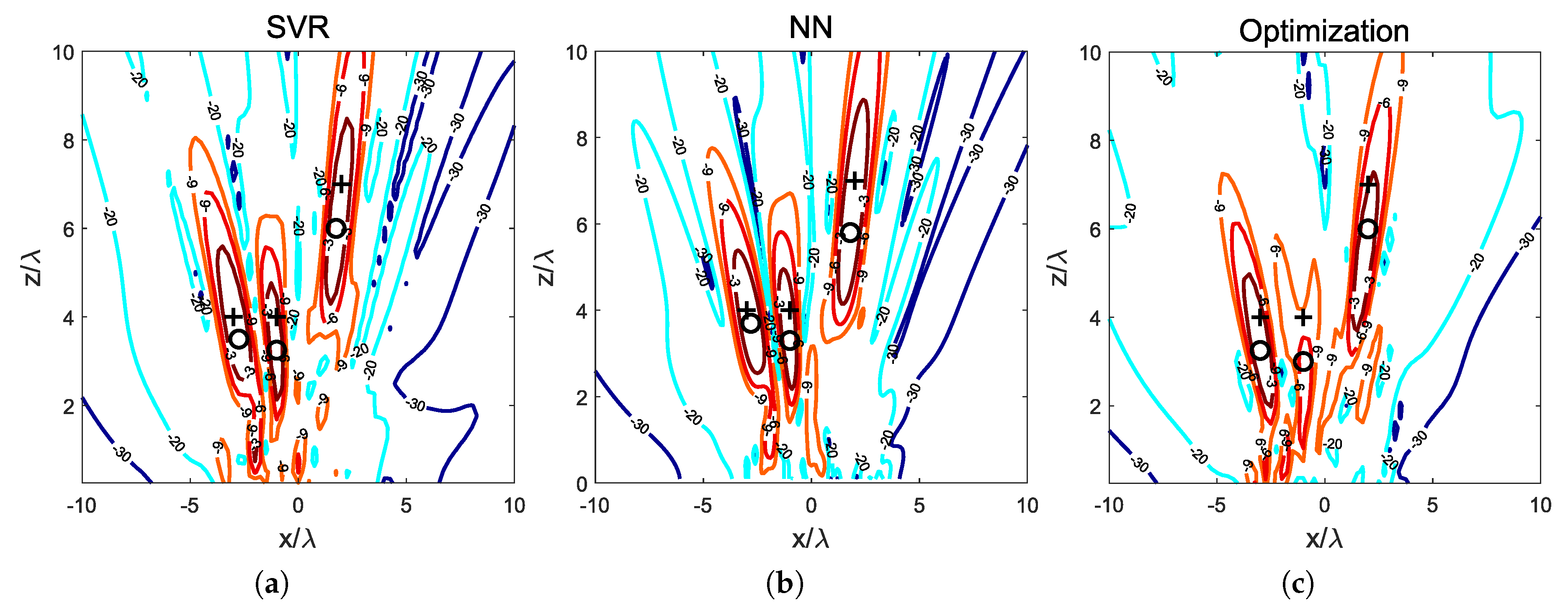
Once the inverse model of the antenna array is obtained, it is used to calculate the weights that must be applied to the array in order to obtain a simultaneous focus on three focal points at $\{x,y,z\}=\{2\lambda ,0,7\lambda \}$, $\{-\lambda ,0,4\lambda \}$ and $\{-3\lambda ,0,4\lambda \}$, to reproduce the experiment presented in [14]. A target field distribution is built using Equation (14), using $C_m=1$ for the assigned focal points and 0 for any other position, and the resulting vector $\mathbf{e}$ is applied to Equation (10). The resulting weights have been used in the MoM model of the antenna to evaluate the resulting radiated field. Figure 1 shows the NF power density distribution in the plane $y=0$ where all the focal points have been specified. The SVR-based model has been able to generate $-3$ dB focal spots containing the three focal points, and spending 0.02 s. The NN presented in [14] and the optimization method proposed in [13] have been used for comparison. The NN-based method has spent 0.19 s for the same problem, while the optimization technique has spent 82.7 s (as stated in [14], this method presents a lower focusing performance as one of the focal points lays out of a $-3$ dB spot with respect to the maximum field power in the NF region). The calculations have been carried out in a conventional PC with an Intel Core i5-7500 CPU, 3.4 GHz and 8 GB RAM, using MatLab R2019a as programming tool, and averaging 20 simulations for all the three methods. Both the SVR- and the NN-based methods spent times suitable for applications with moving devices, but the NN has required 5000 training pairs and the SVR has used 120 pairs to achieve similar performance and faster operation.

The assigned focal points are shown in Figure 1 along with the resulting synthesized spots and the points where the radiated field power is actually maximum. For comparison purposes, the results obtained in [13,14] have been reproduced. The proposed SVR model generates a solution with an NF distribution with the three assigned focal points into $-3$ dB spots, and maximum values of radiated field power density at the positions $\{1.8\lambda ,0,6\lambda \}$, $\{-\lambda ,0,3.3\lambda \}$ and $\{-2.8\lambda ,0,3.65\lambda \}$. These points are located at an average distance of $0.7\lambda$ from the assigned focal points. The NN method outputs a set of weights corresponding to an NF distribution with three maxima located in the positions $\{1.8\lambda ,0,5.8\lambda \}$, $\{-1\lambda ,0,3.3\lambda \}$ and $\{-2.8\lambda ,0,3.7\lambda \}$, with an average distance $0.75\lambda$ between the assigned focal points and the actual maximum points. The optimization method, not accounting for coupling effects, provides a set of weights that correspond to a radiated NF distribution with $-3$ dB spots including only two of the three assigned focal points; its maximum points are located at the positions $\{2\lambda ,0,6\lambda \}$, $\{-\lambda ,0,3\lambda \}$ and $\{-3\lambda ,0,3.25\lambda \}$ with an average distance to the assigned focal points $0.91\lambda$, considering also the focal point out of the $-3$ dB spot. The size of the resulting $-3$ dB spots is summarized in

Table 1. Example #1. Axis length (major, minor) using SVR, neural networks (NN) and optimization (non-coupling).

Focal Point	$\{2\mathit{\lambda },0,7\mathit{\lambda }\}$	$\{-\mathit{\lambda },0,4\mathit{\lambda }\}$	$\{-3\mathit{\lambda },0,4\mathit{\lambda }\}$
Axis length SVR	$3.95\lambda ,0.99\lambda$	$2.54\lambda ,1.09\lambda$	$3.10\lambda ,1.02\lambda$
Axis length NN	$4.85\lambda ,1.22\lambda$	$2.74\lambda ,0.84\lambda$	$2.97\lambda ,0.94\lambda$
Axis length Opt	$3.53\lambda ,1.09\lambda$	no	$3.21\lambda ,0.92\lambda$

.

From these results it may be observed that the use the use of training patterns obtained including the realistic properties of the array leads to improved focusing accuracy without requiring complicated formulations. This is actually one of the main advantages of using machine learning tools for the modeling of the array.

In order to verify the ability of the proposed method to deal with different sizes of arrays, the number of elements of the array has been increased to $32\times 32$ elements, and the interelement distance has been set to $0.7\lambda$ so that the resulting aperture is reasonably larger than the first structure, and hence its focusing capabilities are increased. All the other properties of the array and its elements remain the same, as well as the specifications. The higher number of degrees of freedom should lead, if properly handled by the method, to better focusing performance. The number of training patterns used to obtain the model is 150, and MoM has been used to calculate them. The hyperparameters of the regression remain $C=1$ and $\epsilon =0.001$. The training process stops with a square mean error of 0.036 and 0.037 for the training and validation sets respectively.

Figure 2 shows the resulting NF distribution at the plane $y=0$ where all the focal points are assigned. Both the focal points and the resulting maxima are also plotted. It may be observed that the field is much more concentrated around the assigned points, and that the accuracy in the location of the maximum power density points is much higher than using the smaller structure. The positions where the maximum power density is found are $\{2\lambda ,0,7\lambda \}$, $\{-\lambda ,0,4\lambda \}$ and $\{-3\lambda ,0,4\lambda \}$, all of them exactly at the positions where the focal points are assigned, resulting in an average distance of 0. The axis lengths for the $-3$ dB spots are summarized in

Table 2. Example #1. Axis length (major, minor) using SVR and a $32\times 32$ element array.

Focal Point	$\{2\mathit{\lambda },0,7\mathit{\lambda }\}$	$\{-\mathit{\lambda },0,4\mathit{\lambda }\}$	$\{-3\mathit{\lambda },0,4\mathit{\lambda }\}$
Axis length SVR $32\times 32$	$1.4\lambda ,0.55\lambda$	$1.25\lambda ,0.5\lambda$	$1.25\lambda ,0.5\lambda$

.

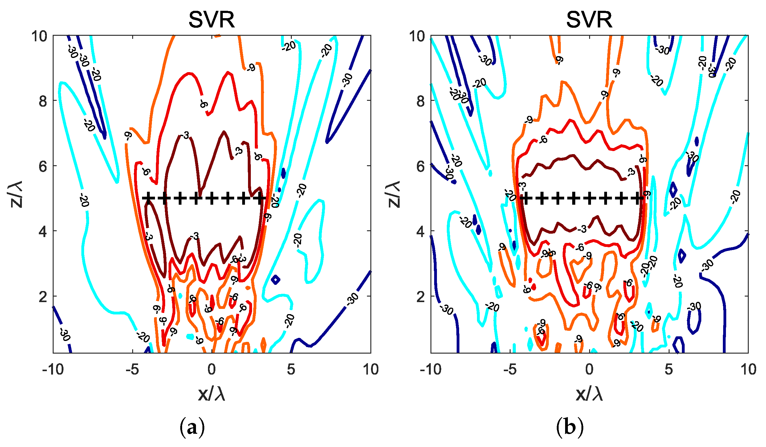
In example #2, a wider coverage area is requested in the NF region of the antenna. To specify it, a set of focal points representing samples of the coverage area has been selected. The assigned focal points are placed at $y=0$, $z=5\lambda$ and $x=[3\lambda ,2\lambda ,\lambda ,0,-\lambda ,-2\lambda ,-3\lambda ,-4\lambda ]$, resulting in eight focal points. In all the cases the corresponding value $C_m$ has been set to 1. The same regular array with $12\times 12$ DRA elements separated $0.6\lambda$ has been considered, operating again at 3.6 GHz. A set of 140 training patterns was obtained using MoM as analysis tool. The hyperparameters of the regression are again $C=1$ and $\epsilon =0.001$. The training process leads to a square mean error of 0.037 and 0.039 for the training and validation sets respectively. The obtained inverse model is used to calculate the set of weights corresponding to the field distribution shown in Figure 3a. It can be observed how a wider region is obtained over $-3$ dB, with all the assigned focal points but one into it. The focal point out of the $-3$ dB spot receives a power density $-3.2$ dB with respect to the maximum power in the NF region. In order to verify that larger arrays have increased focusing capabilities, the number of elements of the array has been increased to $16\times 16$, and the interelement distance has been set to $0.7\lambda$, again to create a larger aperture. The resulting field distribution is plotted in Figure 3b, where the coverage area can be observed clearly defined in a $-3$ dB spot containing all the assigned focal points.

5. Discussion

A machine learning approach to near-field focusing based on the powerful and elegant support vector machines framework is presented. Support vector regression is performed to develop an accurate NF inverse model of a given antenna array. It is calculated from a set of training patterns consisting on known pairs of weights applied to the array elements and the corresponding NF distribution. These patterns may be obtained through measurements or simulation. The necessary number of patterns is strongly reduced with respect to other ML alternatives such as neural networks, due the increased learning capabilities of SVM techniques.

Once the model has been obtained, it can be used for synthesis of focused distributions by following a simple strategy, and without relevant computational cost or time, as synthesis becomes a simple matrix-vector product. The resulting method is suitable for applications requiring fast synthesis to operate in scenarios where real-time calculations are required, for example where moving devices in a near environment are involved (e.g., 5G femtocells, Internet of things, etc.). Although the most popular approach to NFF, conjugate-phase, is very fast, simple and accurate, it cannot deal with multiple specifications; an optimization method, able to account for multifocus requirements, is not fast enough to be used in real-time applications due to its iterative nature; the NN approach is able to be accurate, fast and deal with multifocus, but requires thousands of training pairs, that might overflow many applications and make impossible the use of measured training data. The proposed SVR method overcomes all these difficulties due to the reduced number of required training patterns, its fast operation once trained, and its ability to deal with NF distributions specified in different ways. Additionally, it is able to account for the real properties of the array (realistic effects, coupling effects, individual radiation patterns, non-uniformities, etc.) provided that the method for generating the training patterns also accounts for all of them.

As a future work to be addressed in future developments, more sophisticated specifications such as a mask or template, phase-only distributions or additional constraints to be considered, may be included in the synthesis scheme; by doing so, the resulting method will become much more flexible and powerful. Meanwhile, SVR represents an interesting step for applications where different devices are involved and located in the near-field region of the antenna, even when some of them are moving.