Application of Reservoir Computing for the Modeling of Nano-Contact Vortex Oscillator

Abstract

The Nano-Contact Vortex Oscillator (NCVO) is a highly nonlinear spintronic device that can depict chaotic and nonchaotic behaviors according to the current flowing through it. The potential use of such a device in the future-generation computing systems requires the knowledge of a realistic model capable of describing its exact dynamics. In this paper, we firstly investigate the behavior of NCVO based on the power spectral analysis. Furthermore, we propose and demonstrate two efficient approaches of reservoir computing for the modeling of such a device. The performances of the proposed models are addressed in two ways. First, the generated time-varying signals are compared with the simulated magnetizations of the NCVO at different operating currents. Then, the power spectral analysis of one of the two models is carried out to examine its overall behavior over the complete DC current operating range and its ability to diagnose chaotic and non-chaotic regimes. The proposed models show quite promising results that can be counted on for further research.

1. Introduction

In the era of the Internet of Things (IoT) and Big Data (BD), a huge amount of data of different types is permanently generated and collected by sensing systems over time. The processing of these data strains the conventional CMOS circuits and systems to respect increasing hard timing requirements while trying to keep the overall power consumption in the very limited power budgets. Due to the increasing thermal issues, some limits of the conventional CMOS designs have already been reached and are at the origin of the new orientations that chip designers took in the last decade: heterogeneous Multiprocessor System-on-Chips (MPSoCs) [1]. Although these design orientations have brought some solutions, they are also at the origin of what we call the dark silicon paradigm [2]: the above mentioned thermal issues and stringent power budgets do not allow fully exploiting the overall computing power of a chip whereby through smart management, some portions of it are forcedly deactivated during its normal functioning. On the other hand, the large amount of data that needs to be processed imposes tight constraints not only on the necessary performances per watt that computing circuits and systems need to supply, but also on their overall energy efficiency.

In order to deal more efficiently with the constant computer efficiency demands and the diminishing technology benefits introduced by the technology scaling (leakage, variations, reliability), new beyond-CMOS emergent technologies must be considered. Many alternatives are being explored to meet these challenges. One of the solutions is to replace silicon with a less dissipative material such as graphene [3] or even to use magnetic materials whose bistable magnetization state and inherent non-volatility can be exploited to build Nanomagnetic Logic (NML) [4]; or their spintronic properties to design bioinspired systems [5]. Other approaches, such as quantum computing, propose to redesign the overall computing architecture where quantum effects are leveraging the obtained computing power, allowing significant speedups of certain algorithms [6]; or memcomputing, where combining memory and computation within a single element requires much less power than in conventional computing systems [7].

Another alternative computing paradigm with growing research interest in the last few decades that exploits the inherent dynamics of highly nonlinear and chaotic systems is chaos based computing [8,9]. The dynamics richness of chaotic systems and their high sensitivity to initial conditions allow generating a myriad of different behaviors as a function of time and can be exploited as a basic block of reconfigurable computing systems [9,10]. In the literature, different examples of circuits and systems exhibiting chaotic behavior can be found [11,12,13]. The vast majority are electronic circuits using nonlinear components. Recently, it has been shown that the physical nano-devices such as spin-torque nano-oscillators can be used as building blocks of neuromorphic systems and are a promising solution for post-beyond-CMOS systems essentially due to their small area footprint and computing capabilities at low energy [5,14]. The Nano-Contact Vortex Oscillator (NCVO) is an electrically controllable nano-device characterized by a highly nonlinear dynamics involving infinite states and is one of the potential candidates for the future-generation computing systems [15]. Depending on the direct bias current and the applied magnetic field, the NCVO can engage a chaotic state or stay in a non-chaotic state. Chaos involves highly nonlinear dynamics that leads to apparent random largely unpredictable signals that are in fact deterministic, but sensitive to the initial conditions [16]. In fact, it has been shown recently [15] that, for a well defined geometry, it is possible to move continuously from a commensurable or stable state to an incommensurable or chaotic state. This easy switching between different regimes is very promising to obtain optimal computational performances [17].

The rich behavior of the NCVO’s dynamics occurring within a single physical device opens perspectives for its potential use as a basic building block in more complex systems. By interconnecting and/or synchronizing these blocks, the reconfigurable logic or neuro-inspired computing properties emerge, which may be highly desirable in many applications. In order to use the NCVO as a basic block, an accurate model is needed. The magnetization dynamics that governs the NCVO operation involves too many degrees of freedom which can only be captured with the use of micro-magnetic simulation tools. However, until now, physics has been helpless so far in finding explicit equations that describe the accurate change in the state of NCVO. Thus, the use of SPICE, VerilogA, or any similar modeling tool becomes impossible due to the lack of an obvious mathematical model. Given the possibility of generating accurate magnetization signals faithfully describing the behavior of the NCVO device in all operation modes, black box approaches (based on the known inputs and outputs) may be considered to model the overall behavior of such a device. In this paper, we resort to Neural Networks (NNs), which seem very appropriate to deal with the NCVO’s nonlinear magnetization oscillations. On the other hand, the time-varying behavior of the NCVO device, depending on the input DC current flowing through it, is at the origin of different time series. Thus, the recurrent NNs, which are data-driven, self-adaptive, and can learn several time series and regenerate them, are very worthy of such a modeling task and are our choice in the presented work.

The rest of this paper is organized as follows: Section 2 first introduces the NCVO, its structure, and the physics behind and the influence of current on its behavior. It also includes a brief description of the conventional methods used for system modeling. In Section 3, we demonstrate the two proposed modeling methods: the echo state network and the conceptor-driven network. The obtained results are all shown and discussed in Section 4. Finally, Section 5 gives the concluding remarks and the future outlook.

2. Background and Related Work

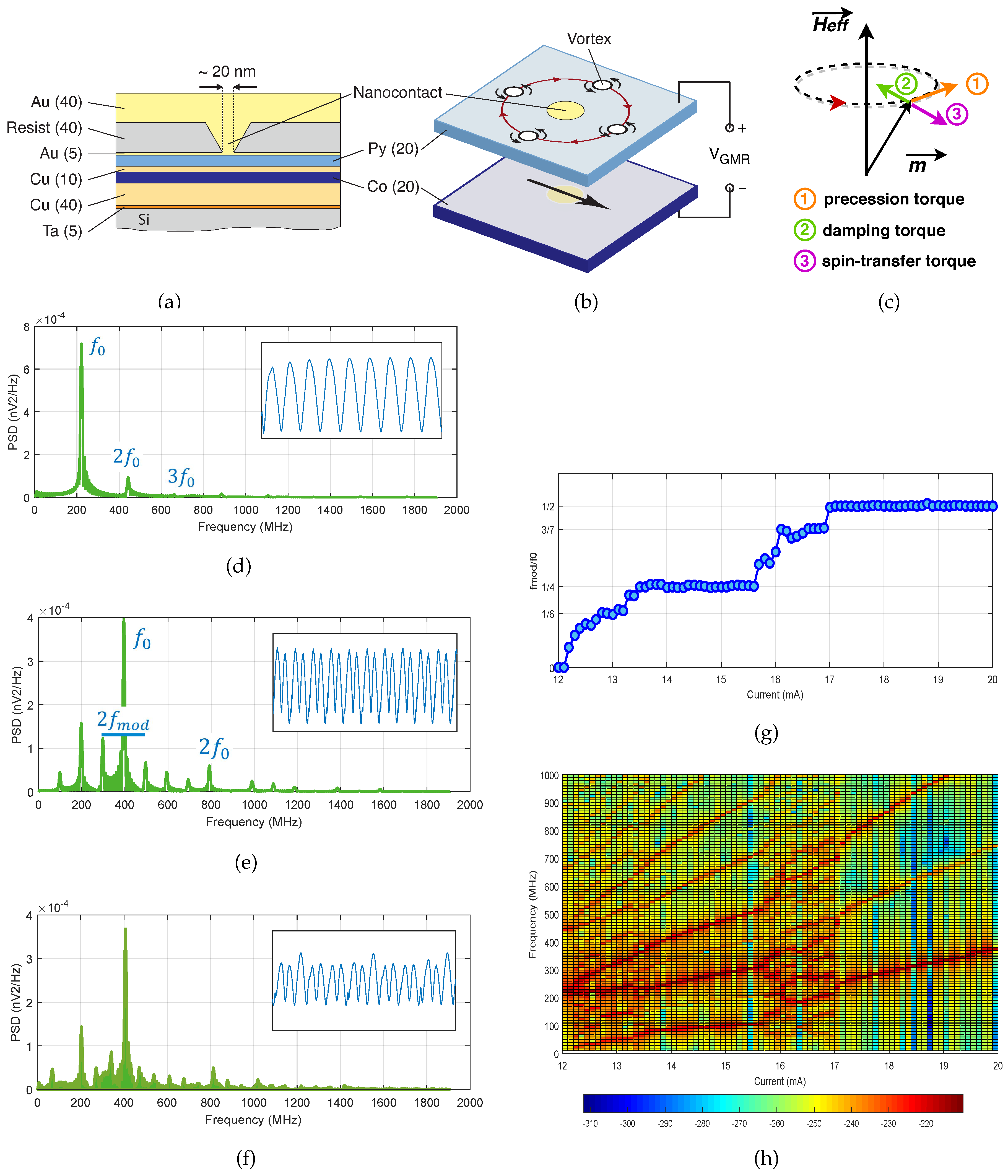
2.1. NCVO and the Physics Behind It

NCVO consists of an extended spin valve structure made of multiple stacked thin layers including two ferromagnetic layers (Figure 1a). The electrical current enters the device through a metallic NanoContact(NC) on top. Most of the flowing currents are perpendicular to the surface, producing a large Oersted–Ampère field with a circulating configuration. This allows the formation of a magnetic vortex only in the upper ferromagnetic layer below the NC. The remaining currents spread in the plane to farther regions and generate a spin transfer torque that moves the vortex core away from the center. At a given distance from the NC, this torque is compensated by a magnetic damping where the combination of these two torques with the precession torque (Figure 1c) leads to a self-sustained gyration of the vortex core around the NC (Figure 1b). In contrast, the magnetization of the lower magnetic cobalt layer remains uniform and is issued as a reference for measuring the Magnetoresistance (MR) of the spin valve. The resistance of the device is then proportional to the azimuthal angle of the vortex core. Since a bias DC current is applied to generate the vortex dynamics, due to the MR effect, an oscillating voltage $V_{GMR}$ at the vortex gyration frequency appears across the device [15].

To study this phenomenon, an NCVO was tested by micro-magnetic simulation for different DC bias current values I while recording the space averaging of the three components of the magnetization vector. For the value I, three different modes are recognized:

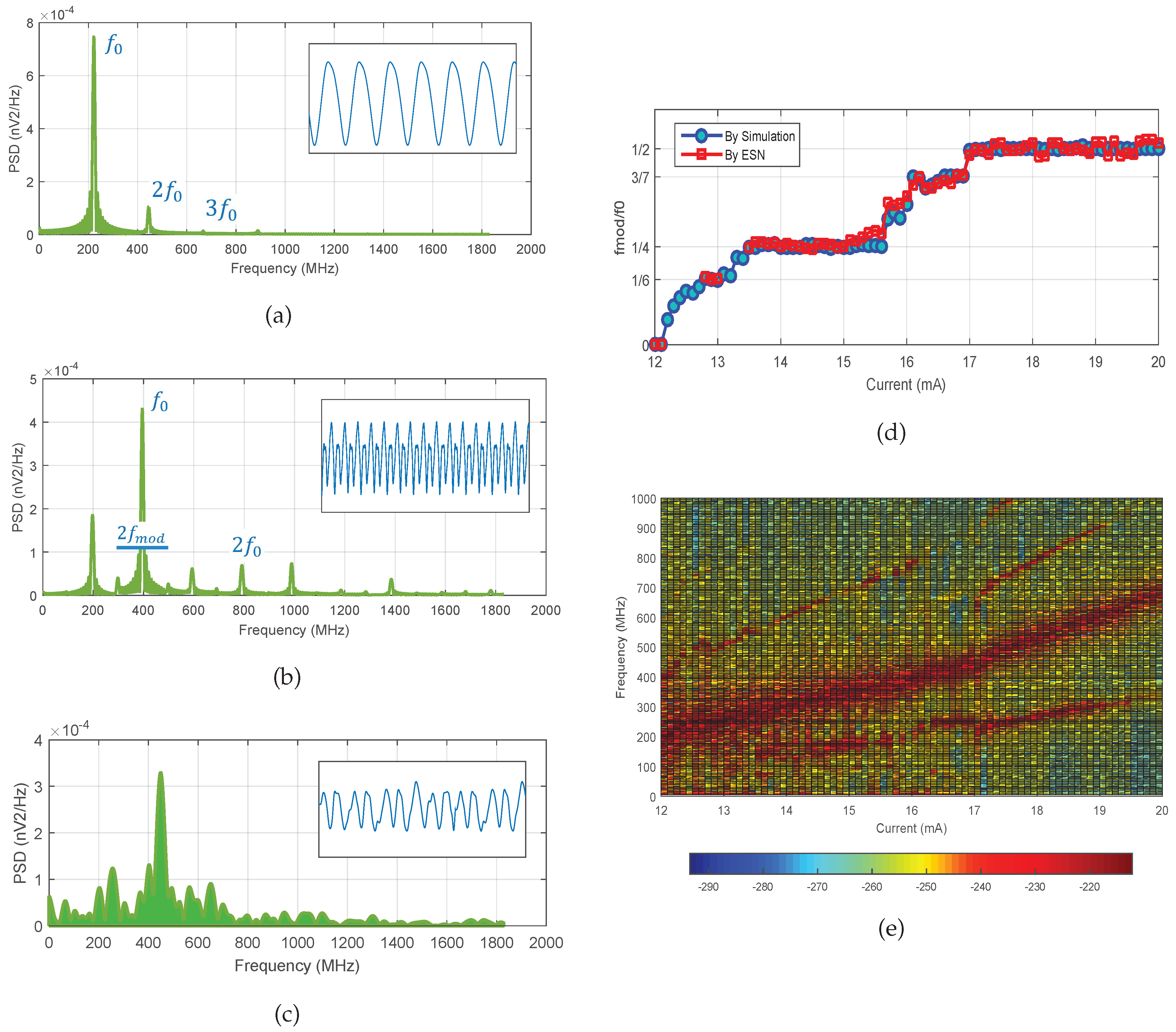
• No-modulation mode: This mode appears for currents I in the range $[12,12.1]$ mA. The vortex revolves around the NC continuously. No change of polarity takes place. Thus, only a fundamental mode, which denotes the gyration frequency, is obtained with its harmonics in the power spectrum (see Figure 1d).
• Modulation mode: This modulation frequency comes from a periodic relaxation of the vortex dynamics due to the core reversal. In this mode, the power spectrum shows two sideband frequencies $\pm f_{mod}$ associated with the gyration frequency $f_0$ (see Figure 1e). $f_{mod}$, which denotes the vortex polarity reversal, is said to be commensurably locked to $f_0$. As a result, the vortex fulfills complete cycles around the NC before dropping toward the center to invert its direction.
• Chaotic mode: As its name indicates, the vortex revolves with no definite rules. The vortex may drop at any time toward the center due to the non-compatibility of the gyration and modulation frequencies (see Figure 1f).

Figure 1g shows the variation of the fraction $f_{mod}/f_0$ as a function of I. The plateaus are a sign of phase-locking phenomenon, whereas the monotonic behavior comes from chaos. To verify this, the power spectrum density is plotted as a function of both the current and frequency (see Figure 1h). At the plateau, only a few frequencies are obtained: the fundamental frequency, its sidebands, and harmonics; whereas in the chaotic region, a large number of frequencies can be observed.

2.2. Modelling Methods

Real-world systems are inherently dynamic and complex. Their complexity is a result of a multitude of factors [18]: dynamic changing of the environment in which systems evolve or of their internal structure; tight coupling and interactions between the parts of systems; feedbacks on the environment dynamics and the system’s; non-linearity giving rise to unpredicted and spontaneous features exhibiting chaos, self-organization, and pattern formation. To model such complex nonlinear systems, different approaches have been proposed in the literature [19,20]. In order to describe the complex dynamics of a system, a common approach is to use nonlinear system identification, consisting of several steps: data acquisition, system model hypothesis, parameter identification, and model test and validation. In the first step, the inputs and the outputs of the system are observed and acquired and will be used throughout all further steps. The system model hypothesis is vital because it needs to describe faithfully the behavior of the observed system, otherwise it will be rejected after the test and validation phases.

Among models used to describe the nonlinear dynamics of a system, different model classes have been reported [20,21,22,23,24,25,26,27]. Continuous-time polynomials represent the first class of models where, by using Ordinary Differential Equations (ODEs), the acquired data can be fitted [21]. The examples of nonlinear models described with ODEs are Lorenz [23] and Rössler systems [24]; the Lotka–Volterra model [28] suited for ecological systems as it efficiently describes the interaction of different species competing in nature [29]; the Kuramoto–Sivashinsky equation for chemical reaction modeling [21]. Complex chaotic dynamics can be modeled as well by delay differential equations [30]. This modeling technique has proven its efficiency in many fields, especially the population dynamics field [31]. Another large class of models used to represent nonlinear dynamics is neural networks [32,33,34]. These networks consist of neurons organized in layers that receive weighted inputs from all other neurons from neighboring layers in a feed-forward manner (no feedback loops) and compute their sum nonlinearly. Such systems can be described with coupled ODEs with a sigmoidal nonlinearity such as the hyperbolic tangent. Their use is well suited for physical problems as a small stimulus produces a linear response that saturates at a given large stimulus. However, the large number of requested parameters makes the system computationally expensive. In contrast to the latter system, sparse neural networks [33] just need a few parameters to mimic a chaotic behavior. The interaction matrices in such networks are circulant [34], corresponding to neurons arranged in a ring, each interacting identically to its neighbors. The main drawback of such networks is the ruinous effect of the initial conditions on the dynamics, which should be defined asymmetrically to avoid synchronization leading to chaos. Other classes of models used to describe the dynamics complexity of nonlinear systems are radial basis function models [35] (similar to NNs without weighted inputs between neurons in hidden layers), fuzzy logic [36], or rational models composed of the division of two polynomials [37].

3. Proposed Models

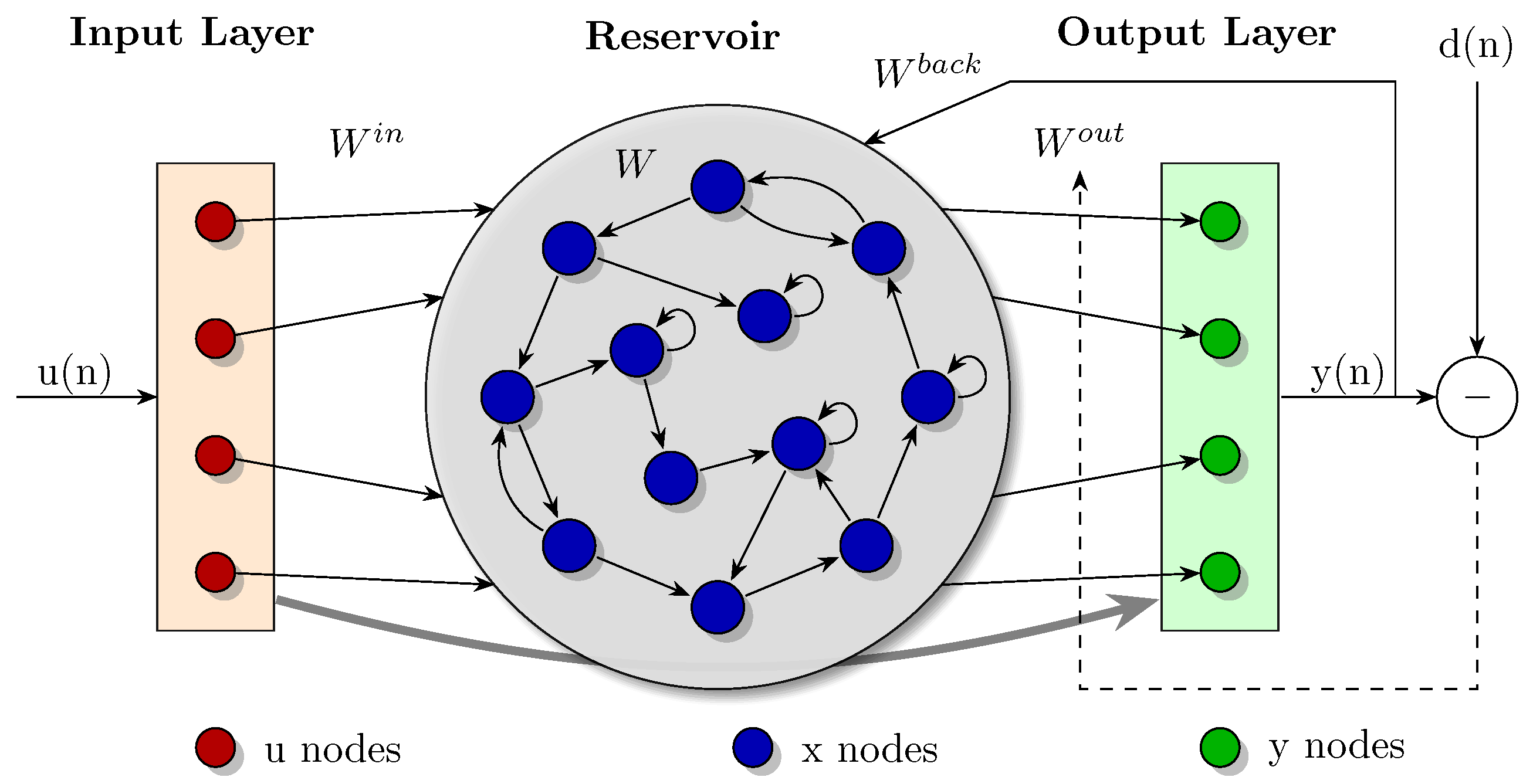
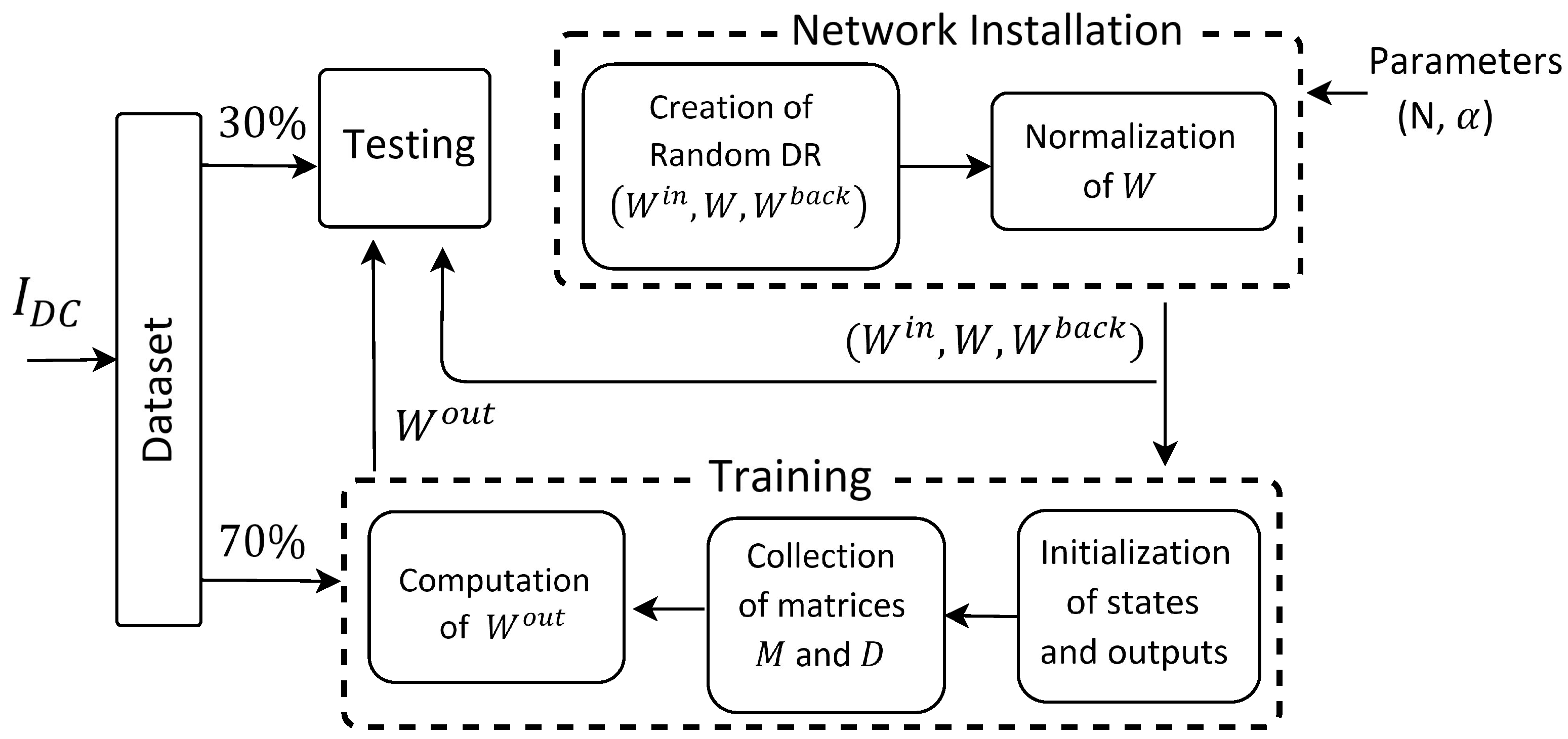
3.1. Echo State Network

The Echo State Network (ESN) approach was first introduced by Herbert Jaeger in 2001 [38]. ESN is composed of K input units u, N internal network units x, and L output units y; combined with a set of weights (Figure 2). After the input data are introduced, the neural network generates its internal states based on the fixed weights: the input matrix $W^{in}$, the internal matrix W, and the backpropagation matrix $W^{back}$. These intermediate values are exploited to train the output connections in the second part of the system: the trainable output matrix $W^{out}$. The first part of the system, known as the reservoir, is a Recurrent Neural Network (RNN), which is not enrolled in the training phase. The second part, called the readout, is a classifying layer usually represented with a simple linear function. The key point in this type of network is the reliance on the input history $u\left(n\right),u(n-1),\cdots ,u\left(0\right)$ for the computation of each internal state $x\left(n\right)$; that is why it is described as “echo”. Knowing that $f=(f_1,..,f_N)$ is the output activation function of internal units, the activation process inside the network follows the following scheme:

$$x(n+1)=f(W^{in}u(n+1)+Wx\left(n\right)+W^{back}y\left(n\right))$$

(1)

On the other side, the output is computed based on the current input, the current internal state, and the previous output values under the output activation function of output units $f^{out}=(f_1^{out},..,f_N^{out})$:

$$y(n+1)=f^{out}\left(W^{out}[u(n+1),x(n+1),y\left(n\right)]\right)$$

(2)

In fact, the “echo state” property of a network is highly related to the internal matrix prepared for training [38,39]. For that, this matrix should be computed carefully, as will be seen later, whereas the remaining matrices of the reservoir can be freely chosen, as they do not affect the echo state property of an ESN.

The construction of the internal reservoir, as well as the output layer is done in the following manner. First, the computation of W is carried out by creating an untrained Dynamic Reservoir (DR) ($W^{in}$, W, $W^{back}$), which has an echo state property and random values for $W^{in}$ and $W^{back}$. The echo state property is ensured by $|{\lambda }_{max}{|}_W<1$, where $|{\lambda }_{max}|$ is the spectral radius of the matrix W corresponding to the largest absolute value of its eigenvalues $\lambda$. The size N of W is generally chosen as $T/10<N<T/2$. This matrix is then multiplied by $(\alpha /|{\lambda }_{max}\left|\right)$ where $\alpha$ is the desired spectral radius of the final matrix W. There are no formal rules for the choice of $\alpha$. However, this parameter can be tuned manually knowing that the large values increase the acceleration of the system’s dynamics [39].

The training phase takes place by initializing the network to an arbitrary state, for example $x\left(0\right)=0$. Then, by setting $y\left(0\right)=0$, the internal states are computed using the activation formula of Equation (1). For $n>T_0$ ($T_0$ is the process washout time): the vector $\left(u\right(n),x(n),y(n-1\left)\right)$ is collected and inserted as a row of matrix M, and the vector ${tanh}^{-1}\left(y\left(n\right)\right)$ is collected and inserted as a new row in the matrix D while going down in rows with time in both matrices.

Finally, the output matrix of the readout layer is calculated by the following equation:

$$W^{out}={\left(M^{-1}D\right)}^T$$

(3)

At this stage, the reservoir ($W^{in}$, W, $W^{back}$, $W^{out}$) is ready for use. It can be tested by computing the internal states Equation (1) and then the output units Equation (2) using the learned weight matrices. The whole process is summarized by a flowchart diagram in Figure 3. The obtained echo state network can be successfully used to model one time series. In the NCVO case, one time series corresponds to one set of magnetization signals ($M_x\left(t\right)$, $M_y\left(t\right)$ and $M_z\left(t\right)$) obtained for one value of the input DC current. Therefore, it becomes impossible to capture all the sets of magnetization signals of the NCVO device using a single system. To do that, separately trained ESNs are needed. In other words, the number of echo state networks should be equal to the number of input datasets. In the next section, we expose a new methodology of training recurrent neural networks, which, by its memory, assures the easy switching of the different input datasets under the same weights. Consequently, the magnetization signals $M_x\left(t\right)$, $M_y\left(t\right)$, and $M_z\left(t\right)$ can be captured at different DC current values, previously trained on, using a single system.

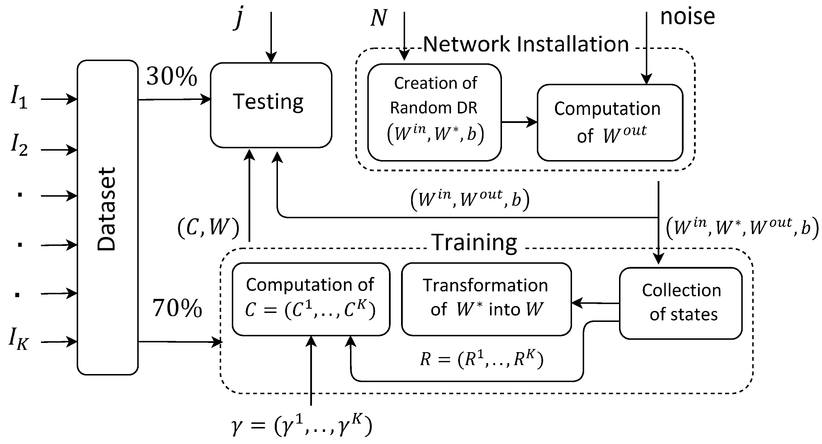
3.2. Conceptors-Driven Network

The behavior of an NCVO varies with respect to the value of the direct current flowing through the device. Thus, there is a need for neural Long-Term Memory (LTM) [40] capable of saving and regenerating a large number of time series patterns. We suggest the use of conceptors-reservoir computing [41], which passes serially through two phases: the loading phase where patterns are installed in the network and the recall phase in which the patterns are regained according to the conceptor’s value.

To model this system, an RNN with N neurons is built by randomly creating an $N\times N$ internal connection matrix $W^{*}$, an $N\times K$ input weights matrix $W^{in}$ where K denotes the number of input datasets, and a N random bias vector b. In the loading phase, the scalar pattern $p^j\left(n\right)$ always drives the network by the following state-update equation:

$$x^j(n+1)=tanh(W^{*}{x}^j\left(n\right)+W^{in}{p}^j\left(n\right)+b)$$

(4)

Note that j denotes the index of the pattern.

Before starting, the network undergoes a training of the readout matrix where an M-dimensional white noise $\nu \left(n\right)$ is introduced to the network to collect the states:

$$x^{\nu }(n+1)=tanh(W^{*}{x}^{\nu }\left(n\right)+W^{in}\nu \left(n\right)+b)$$

(5)

Accordingly, $W^{out}$ is computed via the optimization problem below:

$$\underset{W^{out}}{\min }\sum _n{(W^{out}{x}^{\nu }\left(n\right)-\nu \left(n\right))}^2$$

(6)

Note that the readout neuron is trained on a random signal, and thus, it should perform well for any temporal signal.

The input internalization weights matrix W is induced from the random matrix $W^{*}$. This transformation enables the new reservoir to mimic the impact of the drivers $p^j$ in the absence of them. For that, the K patterns are fed into the reservoir by separate runs to compute the states $x^j$ according to Equation (4) for $1⩽j⩽K$. Consequently, W is calculated by minimizing the quadratic loss of Equation (7) after the washout period $n_0$ ends:

$$\sum _{j=1,..K}\sum _{n=n_0,..L}{\parallel W^{*}{x}^j\left(n\right)+W^{in}{p}^j\left(n\right)-W{x}^j\left(n\right)\parallel }^2$$

(7)

Although, if the network is run just by iterating $x(n+1)=tanh\left(Wx\right(n)+b)$, the resulting input-free reservoir dynamics is entirely unpredictable. The basic role of the conceptors in the LTM is to guide the system to which temporal pattern it should engage at the exploitation time. Conceptors are $N\times N$ matrices, which interfere in the following manner:

$$x^j(n+1)=C^{j}tanh(W{x}^j\left(n\right)+b)$$

(8)

By referring to [41], the quadratic loss function for the computation of the matrices $C^{j}s$ is:

$$L\left(C^j\right)=E\parallel C^j{x}^j\left(n\right)-x^j\left(n\right){\parallel }^2+{\left({\gamma }^j\right)}^{-2}{\parallel C^j\parallel }_{fro}^2$$

(9)

and its explicit solution is as follows:

$$C^j=R^j{(R^j+{\left({\gamma }^j\right)}^{-2}I)}^{-1}$$

(10)

where $R^j=E\left[x^j\left(n\right)x^j{\left(n\right)}^T\right]$ is the $N\times N$ correlation matrix of states $x^j\left(n\right)$, ${\parallel .\parallel }_{fro}^2$ denotes the squared Frobenius matrix norm, and $\gamma$ is the aperture parameter that can be understood as a virtual scaling factor of the reservoir states. Note that $R^j$ is computed first without the intervention of the conceptors Equation (4). Afterwards, conceptor $C^j$ is calculated easily by Equation (10). This is done for each pattern separately.

After the RNN is completely installed, it enters the recall phase. At this stage, the system is able to obtain any pattern’s state using its conceptor in the following sense:

$$x(n+1)=C^{j}tanh(Wx\left(n\right)+b)$$

(11)

The final output is computed linearly from the network state through the readout weight matrix $W^{out}$:

$$y\left(n\right)=W^{out}x\left(n\right)\approx p\left(n\right)$$

(12)

This process is summarized in Figure 4 as a flowchart diagram.

4. Results and Discussion

4.1. Simulation Setup

The reference signals for training of both proposed models were obtained from the finite difference micromagnetic solver Mumax3 [42], which performs a numerical space and time integration of the Landau–Lifshitz–Gilbert equation including the different spin transfer torque terms. The mesh was composed of 512 cells in each of the x and y directions and one cell in the z direction (along the depth of the ferromagnetic layer). The cell size used was $2.5\times 2.5$ $\mathsf{\mu }$m${}^2$ in the film plane (x and y direction) and 20 nm for the thickness. The current distribution and the Oersted field it generates were previously calculated with COMSOL [43], before being injected as a parameter in Mumax3. A precise description of the procedure used to realize these simulations can be found in the Supplementary Section in [15] and in [44]. The extracted $M_x\left(t\right)$ and $M_y\left(t\right)$ correspond to the time evolution of the average magnetization along the x and y directions, respectively. The measured signal on a real device is proportional to a linear combination of these two quantities. For the modeling work, the two approaches of RC were executed on the simulated data by running a programming code on MATLAB R2015a.

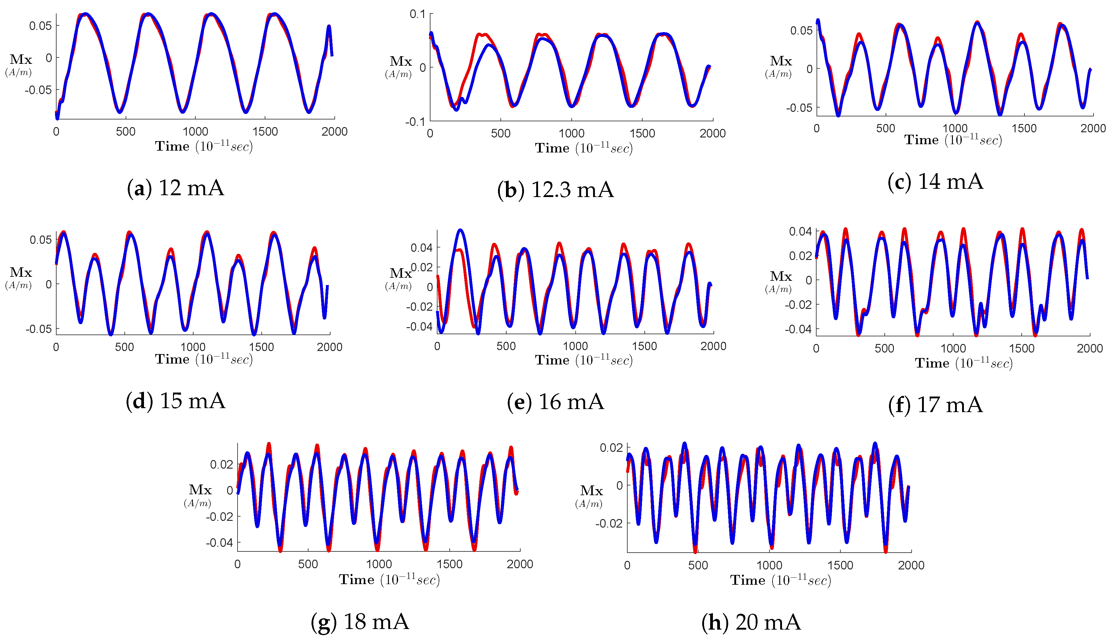
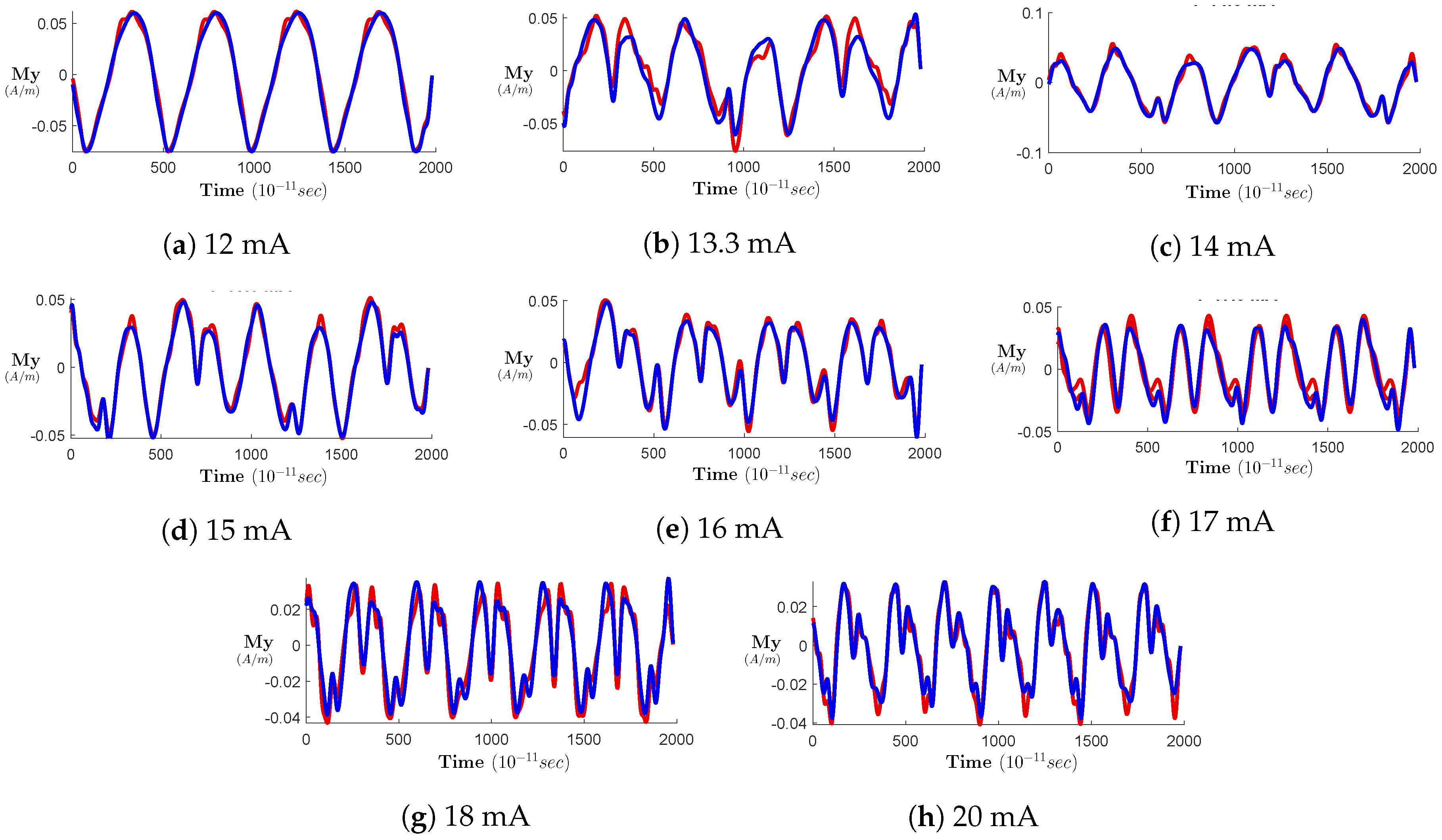
4.2. Generated Data from the Proposed Models

In this subsection, we present the dynamics generated by both the ESN and conceptors-driven RNN, presented in the two previous sections and try to depict the real dynamic magnetizations of NCVO (see Section 4.1). The data we processed were the spatial averaging of the two in-plane components of the NCVO’s outputted magnetization ($M_x$ and $M_y$) obtained from micro-magnetic simulations and considered here as gold reference signals (see Section 4.1). The third dimension of magnetization was not studied as it only denotes the vortex polarity. The injected current ranged from 12 mA to 20 mA with a step of $0.1$ mA. Therefore, by varying the injected current with a $0.1$ mA step in the [12 mA, 20 mA] range in the micro-magnetic simulation framework, we obtained 81 reference datasets, which were further used for the training of both the ESN and conceptor-driven approaches. Each of the 81 input datasets had a data length of T = 10,000 samples with a time step $t_s={10}^{-11}$. The hyperparameter tuning of the ESN approach was done as in [45].

For the ESN, the number of neurons was set to 3000, and the spectral radius $\alpha$ was tuned for each input current separately. Seventy percent of the data was used for training, and the rest was left for testing. Some of the obtained results with this approach of different waveforms are shown in Figure 5 and Figure 6 for both $M_x$ and $M_y$, respectively. At $I=12$ mA no modulation was captured; at I = 12.3 mA, 13.3 mA, and 16 mA, the system was said to be chaotic; and for the rest, it was non-chaotic.

On the contrary, the 3000 neuron conceptors-driven RNN was filled with the 81 training examples $p^j\left(n\right)$ one after the other before the regeneration phase. The conceptor $C^j$ of each pattern was computed after tuning its aperture ${\alpha }^j$. Thirty percent of the data length was dedicated for the recall phase. Similarly, the obtained results with this approach are shown in Figure 7 and Figure 8 for both $M_x$ and $M_y$, respectively.

At first glance, the two networks provided good tracking results in three modes: no-modulation, modulation, and even in the chaotic regime. The latter behavior occurred at $12.3$ mA, $13.3$ mA, and 16 mA, where the time-varying signals were slightly distorted. In all figures, the signals generated by the ESN and conceptor-driven RNN are presented in red, whereas the signals issued from the micro-magnetic simulations of the NCVO are in blue. In order to evaluate the tracking results of both approaches, a comparison in terms of the Mean Squared Error (MSE) between the generated signals obtained on testing data and reference signals (from micro-magnetic simulations) was carried out. These results are shown in

Table 1. Comparison between the conceptor-driven NN and ESN generated signals obtained on testing data in terms of the MSEof $M_x$ and $M_y$ with the reference signals from micro-magnetic simulations.

	MSE of ${\mathit{M}}_{\mathit{x}}$		MSE of ${\mathit{M}}_{\mathit{y}}$
I (mA)	Conceptor-Driven	ESN	Conceptor-Driven	ESN
12	$2.032\times {10}^{-5}$	$7.07\times {10}^{-6}$	$2.36\times {10}^{-5}$	$2.69\times {10}^{-6}$
$12.3,13.3$	$2.24\times {10}^{-4}$	$1.37\times {10}^{-4}$	$9.5713\times {10}^{-5}$	$3.37\times {10}^{-5}$
13	$7.08\times {10}^{-4}$	$\mathrm{3.9\; 5}\times {10}^{-4}$	$5.29\times {10}^{-4}$	$4.75\times {10}^{-4}$
14	$1.86\times {10}^{-4}$	$4.65\times {10}^{-5}$	$2.07\times {10}^{-5}$	$7.22\times {10}^{-5}$
15	$6.7\times {10}^{-5}$	$2.88\times {10}^{-5}$	$1.52\times {10}^{-5}$	$4.33\times {10}^{-5}$
16	$1.16\times {10}^{-4}$	$7.03\times {10}^{-5}$	$3.35\times {10}^{-5}$	$2.13\times {10}^{-4}$
17	$4.16\times {10}^{-5}$	$3.37\times {10}^{-5}$	$3.83\times {10}^{-5}$	$2.82\times {10}^{-5}$
18	$3.41\times {10}^{-5}$	$1.52\times {10}^{-6}$	$4.92\times {10}^{-5}$	$1.02\times {10}^{-5}$
19	$5.89\times {10}^{-5}$	$9.37\times {10}^{-6}$	$2.29\times {10}^{-5}$	$5.29\times {10}^{-6}$
20	$1.99\times {10}^{-5}$	$3.01\times {10}^{-6}$	$2.42\times {10}^{-5}$	$8.6\times {10}^{-6}$

. It can be noticed that the MSE for all currents for both magnetizations and approaches was in the $[{10}^{-4},{10}^{-7}]$ range. However, the ESN approach seemed more accurate for most of the current range for both magnetizations when compared to the reference signals from micro-magnetic simulations. This result was expected as for each current, the parameters of the ESN network were tuned separately to allow better tracking of the NCVO magnetizations corresponding to that current. However, the main drawback of this approach was that it was able to generate only one output signal per run. On the other hand, the conceptor-driven RNN approach gave comparable and for some currents even better tracking results when the generated signals on the testing data were compared with the reference ones from micro-magnetic simulations. Moreover, it had the advantage that once the network was trained, it could be used for all currents to generate the output signals only by changing the conceptor value.

As the ESN approach generated more accurate traces in terms of MSE when compared with the micro-magnetic reference signals, the generated results from testing data were also compared with these reference signals in terms of power spectral analysis. These results are shown in Figure 9. Figure 9e shows the power spectral densities for all observed DC currents in a 2D plot. Thus, for a given DC current, all frequencies generated by the proposed ESN model from testing data can be observed on the PSD color map along the vertical axis. For instance, the power spectra corresponding to three different DC currents generated by the ESN model from testing data are presented in Figure 9a–c for $I=12$, $15.3$, and $16.2$ mA, respectively. These three different currents correspond to the three previously identified operation modes of the NCVO device. For 12 mA, only the fundamental frequency $f_0$, corresponding to the NCVO gyration frequency, and its harmonics are observed. As explained in Section 2.1, this power spectrum is characteristic for the no-modulation regime of the NCVO device. For $15.3$ mA, besides the fundamental frequency $f_0$ and its harmonics, the modulation frequency sidebands $f_{mod}$ can be visualized. Referring to Section 2.1, the modulation mode of the NCVO was identified from this power spectrum. Finally, for $16.2$ mA, a frequency rich power spectrum was observed, which was characteristic of the third chaotic and incommensurable regime. Therefore, all three regimes of the NCVO described in Section 2.1 were all captured by the ESN model.

This plot extracted from the signals generated by the ESN model (in red) was compared with the $f_{mod}/f_0$ of the reference system from micro-magnetic simulations (in blue) and is shown in Figure 9d. In the $f_{mod}/f_0$ plot, the plateaus are signs of the synchronization regions where the NCVO device can be either in no-modulation or modulation mode. Moreover, each plateau was described with a rational number indicating the number of turns of the NCVO vortex before changing the polarity. On the other hand, the monotonic rate in the $f_{mod}/f_0$ plot indicates non-stable and chaotic regions. By comparing the results presented in Figure 9, it can be noticed that the non-chaotic regions are still distinguished in the results generated by the ESN model where the value of $f_{mod}/f_0$ in the intervals $[12.9,13]$ mA, $[13.5,15.6]$ mA, and $[17,20]$ mA varies slightly around $1/6$, $1/4$, and $1/2$, respectively. This means that the ESN model clearly distinguishes the modulation mode of the NCVO device (see Section 2.1). Moreover, the monotonic rates captured by the ESN model between these non-chaotic regions or plateaus are the sign of the chaotic mode behavior. On the other side, it can be noticed that the sideband frequencies cannot be extracted for some DC current values; these frequencies belong to the regions where chaos is dominant. This can be noticed in the 2D plot of PSD (Figure 9e), where for I belonging to the interval $[12.2,13.4]$ mA, the lower sideband frequency cannot be easily identified. Moreover, from Figure 9e, it can also be seen that the presented ESN modeling approach filters the harmonics of the gyration frequency, which are clearly visible in the PSD plot from micro-magnetic simulations presented in Figure 1.

In addition, to confirm the validity of the proposed ESN model to capture the time-varying nonlinear dynamics of the NCVO device along the whole DC current range, another way of presenting its generated PSD results from testing data is to plot the $f_{mod}/f_0$ curve.

5. Conclusions

In the present work, two different modeling approaches were applied to model and describe the complex highly nonlinear dynamics of the spintronic device called the Nano-Contact Vortex Oscillator (NCVO). The behavior of this NCVO device can be controlled with the input DC current flowing though it and can be chaotic or nonchaotic with clearly identified frequency patterns. Two different reservoir computing based approaches were considered: the echo state network method was used to describe the NCVO’s behavior for each DC current; and conceptor-based reservoir computing for all possible DC currents. Both modeling approaches gave good tracking results of the generated signals when compared with the simulated signals from micro-magnetic simulations with the MSE error in the range of $[{10}^{-4},{10}^{-7}]$. The proposed ESN model generated from testing data more accurate results than the conceptor-based reservoir computing approach, but at the detriment of the system’s complexity. Indeed, in the proposed ESN approach, one NCVO’s state, which corresponds to one DC current, was described with a different ESN trained separately. On the other hand, the conceptor-based reservoir computing approach gave comparable and for some currents even better tracking results and had the advantage that once trained, it could be used for all DC currents only by changing the conceptor value. Moreover, the performances of the ESN approach were also compared with the simulation results from micro-magnetic simulations in terms of the power spectral density and $f_{mod}/f$ as a function of the applied DC current. The obtained results showed that the proposed modeling approaches allowed faithfully approximating the complex behavior of the NCVO device and gave quite promising insights for their future use as a basic block in future generation computing systems. Future work should consider the use of the proposed models as a building block of more complex computing systems.

References

1. Wolf, W.; Jerraya, A.; Martin, G. Multiprocessor system-on-chip (mpsoc) technology. IEEE Trans. Comput.-Aided Des. Integr. Circuits Syst. 2008, 27, 1701–1713. [Google Scholar] [CrossRef]
2. Taylor, M.B. A landscape of the new dark silicon design regime. IEEE Micro 2013, 33, 8–19. [Google Scholar] [CrossRef]
3. Sharbati, M.T.; Du, Y.; Torres, J.; Ardolino, N.D.; Yun, M.; Xiong, F. Low-power, electrochemically tunable graphene synapses for neuromorphic computing. Adv. Mater. 2018, 30, 1802353. [Google Scholar] [CrossRef] [PubMed]
4. Eichwald, I.; Breitkreutz, S.; Ziemys, G. György Csaba, Wolfgang Porod, and Markus Becherer. Majority logic gate for 3d magnetic computing. Nanotechnology 2014, 25, 335202. [Google Scholar] [CrossRef] [PubMed]
5. Grollier, J.; Querlioz, D.; Stiles, M.D. Spintronic nanodevices for bioinspired computing. Proc. IEEE 2016, 104, 2024–2039. [Google Scholar] [CrossRef] [PubMed]
6. Castelvecchi, D. Quantum computers ready to leap out of the lab in 2017. Nat. News 2017, 541, 9. [Google Scholar] [CrossRef]
7. Di Ventra, M.; Pershin, Y.V. Just add memory. Sci. Am. 2015, 312, 56–61. [Google Scholar] [CrossRef]
8. Kuo, D. Chaos and its computing paradigm. IEEE Potentials 2005, 24, 13–15. [Google Scholar] [CrossRef]
9. Kia, B.; Kia, S.; Lindner, J.F.; Sinha, S.; Ditto, W.L. Noise tolerant spatiotemporal chaos computing. Chaos Interdiscip. J. Nonlinear Sci. 2014, 24, 043110. [Google Scholar] [CrossRef]
10. Beyki, M.; Yaghoobi, M. Chaotic logic gate: A new approach in set and design by genetic algorithm. Chaos Solitons Fractals 2015, 77, 247–252. [Google Scholar] [CrossRef]
11. Piper, J.R.; Sprott, J.C. Simple autonomous chaotic circuits. IEEE Trans. Circuits Syst. II Express Briefs 2010, 57, 730–734. [Google Scholar] [CrossRef]
12. Tchitnga, R.; Nguazon, T.; Louodop Fotso, P.H.; Gallas, J.A.C. Chaos in a single op-amp–based jerk circuit: Experiments and simulations. IEEE Trans. Circuits Syst. II Express Briefs 2015, 63, 239–243. [Google Scholar] [CrossRef]
13. Srisuchinwong, B.; Munmuangsaen, B.; Ahmad, I.; Suibkitwanchai, K. On a simple single-transistor-based chaotic snap circuit: A maximized attractor dimension at minimized damping and a stable equilibrium. IEEE Access 2019, 7, 116643–116660. [Google Scholar] [CrossRef]
14. Yogendra, K.; Fan, D.; Shim, Y.; Koo, M.; Roy, K. Computing with coupled spin torque nano oscillators. In Proceedings of the 2016 21st Asia and South Pacific Design Automation Conference (ASP-DAC), Macau, China, 25–28 January 2016; pp. 312–317. [Google Scholar]
15. Petit-Watelot, S.; Kim, J.-V.; Ruotolo, A.; Otxoa, R.M.; Bouzehouane, K.; Grollier, J.; Vansteenkiste, A.; Van de Wiele, B.; Cros, V.; Devolder, T. Commensurability and chaos in magnetic vortex oscillations. Nat. Phys. 2012, 8, 682. [Google Scholar] [CrossRef]
16. Pathak, J.; Lu, Z.; Hunt, B.R.; Girvan, M.; Ott, E. Using machine learning to replicate chaotic attractors and calculate lyapunov exponents from data. Chaos Interdiscip. J. Nonlinear Sci. 2017, 27, 121102. [Google Scholar] [CrossRef]
17. Legenstein, R.; Maass, W. What makes a dynamical system computationally powerful. In New Directions in Statistical Signal Processing: From Systems to Brain; MIT Press: Cambridge, MA, USA, 2007; pp. 127–154. [Google Scholar]
18. Sterman, J.D. System dynamics modeling: tools for learning in a complex world. Calif. Manag. Rev. 2001, 43, 8–25. [Google Scholar] [CrossRef]
19. Aguirre, L.A.; Letellier, C. Modeling nonlinear dynamics and chaos: A review. In Mathematical Problems in Engineering; Hindawi: London, UK, 2009. [Google Scholar]
20. Strogatz, S.H. Nonlinear Dynamics and Chaos: With Applications to Physics, Biology, Chemistry, and Engineering; CRC Press: Boca Raton, FL, USA, 2018. [Google Scholar]
21. Volos, C.; Akgul, A.; Pham, V.; Stouboulos, I.; Kyprianidis, I. A simple chaotic circuit with a hyperbolic sine function and its use in a sound encryption scheme. Nonlinear Dyn. 2017, 89, 1047–1061. [Google Scholar] [CrossRef]
22. Hénon, M. A two-dimensional mapping with a strange attractor. In The Theory of Chaotic Attractors; Springer: Berlin, Germany, 1976; pp. 94–102. [Google Scholar]
23. Yang, Q.; Bai, M. A new 5d hyperchaotic system based on modified generalized lorenz system. Nonlinear Dyn. 2017, 88, 189–221. [Google Scholar] [CrossRef]
24. Laiphrakpam, D.S.; Khumanthem, M.S. Cryptanalysis of symmetric key image encryption using chaotic rossler system. Optik 2017, 135, 200–209. [Google Scholar] [CrossRef]
25. Boccara, N. Modeling complex systems. In Modeling Complex Systems: Graduate Texts in Contemporary Physics; Springer-Verlag New York, Inc.: New York, NY, USA, 2004; ISBN 978-0-387-40462-2. [Google Scholar]
26. Lewin, R. Complexity: Life at the Edge of Chaos; University of Chicago Press: Chicago, IL, USA, 1999. [Google Scholar]
27. Bar-Yam, Y. Dynamics of Complex Systems; CRC Press: Boca Raton, FL, USA, 2019. [Google Scholar]
28. Murray, J.D. Mathematical Biology, 2nd ed.; Springer: Berlin, Germany, 1993. [Google Scholar]
29. Hardin, G. The competitive exclusion principle. Science 1960, 131, 1292–1297. [Google Scholar] [CrossRef]
30. Bellen, A.; Zennaro, M. Numerical Methods for Delay Differential Equations; Oxford University Press: Oxford, UK, 2003. [Google Scholar]
31. Zuniga-Aguilar, C.J.; Coronel-Escamilla, A.; Gomez-Aguilar, J.F.; Alvarado-Martinez, V.M.; Romero-Ugalde, H.M. New numerical approximation for solving fractional delay differential equations of variable order using artificial neural networks. Eur. Phys. J. Plus 2018, 133, 75. [Google Scholar] [CrossRef]
32. Sompolinsky, H.; Crisanti, A.; Sommers, H.-J. Chaos in random neural networks. Phys. Rev. Lett. 1988, 61, 259. [Google Scholar] [CrossRef] [PubMed]
33. Derrida, B.; Gardner, E.; Zippelius, A. An exactly solvable asymmetric neural network model. EPL (Europhys. Lett.) 1987, 4, 167. [Google Scholar] [CrossRef]
34. Gray, R.M. Toeplitz and circulant matrices: A review. Found. Trends Commun. Inf. Theory 2006, 2, 155–239. [Google Scholar] [CrossRef]
35. Han, H.-G.; Guo, Y.-N.; Qiao, J.-F. Nonlinear system modeling using a self-organizing recurrent radial basis function neural network. Appl. Soft Comput. 2018, 71, 1105–1116. [Google Scholar] [CrossRef]
36. Xing, F.Z.; Cambria, E.; Zou, X. Predicting evolving chaotic time series with fuzzy neural networks. In Proceedings of the 2017 International Joint Conference on Neural Networks (IJCNN), Anchorage, AK, USA, 14–19 May 2017; pp. 3176–3183. [Google Scholar]
37. Din, Q.; Elsadany, A.A.; Ibrahim, S. Bifurcation analysis and chaos control in a second-order rational difference equation. Int. J. Nonlinear Sci. Numer. Simul. 2018, 19, 53–68. [Google Scholar] [CrossRef]
38. Jaeger, H. The “echo state” approach to analysing and training recurrent neural networks-with an erratum note. Bonn Ger. Ger. Natl. Res. Cent. Inf. Technol. GMD Tech. Rep. 2001, 148, 13. [Google Scholar]
39. Jaeger, H. Tutorial on Training Recurrent Neural Networks, Covering BPPT, RTRL, EKF and the “Echo State Network” Approach; GMD-Forschungszentrum Informationstechnik: Bonn, Germany, 2002; Volume 5. [Google Scholar]
40. Furlanello, T.; Zhao, J.; Saxe, A.M.; Itti, L.; Tjan, B.S. Active Long Term Memory Networks. arXiv 2016, arXiv:1606.02355. [Google Scholar]
41. Jaeger, H. Using conceptors to manage neural long-term memories for temporal patterns. J. Mach. Learn. Res. 2017, 18, 387–429. [Google Scholar]
42. Vansteenkiste, A.; Leliaert, J.; Dvornik, M.; Helsen, M.; Garcia-Sanchez, F.; Van Waeyenberge, B. The design and verification of mumax3. AIP Adv. 2014, 4, 107133. [Google Scholar] [CrossRef]
43. Petit-Watelot, S.; Otxoa, R.M.; Manfrini, M. Electrical properties of magnetic nanocontact devices computed using finite-element simulations. Appl. Phys. Lett. 2012, 100, 083507. [Google Scholar] [CrossRef]
44. Létang, J.; Petit-Watelot, S.; Yoo, M.-W.; Devolder, T.; Bouzehouane, K.; Cros, V.; Kim, J.-V. Modulation and phase-locking in nanocontact vortex oscillators. arXiv 2019, arXiv:1906.08492. [Google Scholar] [CrossRef]
45. Lukoševičius, M. A practical guide to applying echo state networks. In Neural Networks: Tricks of the Trade; Springer: Berlin, Germany, 2012; pp. 659–686. [Google Scholar]
Figure 1. Micro-magnetic simulation: (a) Multilayer composition of the pseudo-spin valve studied, with the layers’ thickness in nanometers and (b) the gyrotropic motion of the vortex in the permalloy (Py) layer, with uniform magnetization in the cobalt layer [15]. (c) Torques acting on the free layer magnetization of NCVO. Measured power spectra and time traces (in the inset) of the magnetization in (d) the no modulation ( I = 12 mA), (e) non-chaotic ( I = 15.3 mA) (f), and chaotic ( I = 16.2 mA) cases. (g) Variation of the ratio between the modulation and central frequencies as a function of the applied current. (h) Color map of the PSD as a function of the current.
Electronics 08 01315 g001
Figure 2. General structure of an echo state network.
Electronics 08 01315 g002
Figure 3. Flowchart diagram of the echo state network.
Electronics 08 01315 g003
Figure 4. Flowchart diagram of conceptor-driven network.
Electronics 08 01315 g004
Figure 5. Variation of M x ( A / m ) versus time ( 10 11 s e c ) for different values of I with the original signal (blue plot) and the signal generated by the Echo State Network (ESN) (red plot).
Electronics 08 01315 g005
Figure 6. Variation of M y ( A / m ) versus time ( 10 11 s e c ) for different values of I with the original signal (blue plot) and the signal generated by ESN (red plot).
Electronics 08 01315 g006
Figure 7. Variation of M x ( A / m ) versus time ( 10 11 s e c ) for different values of I with the original signal (blue plot) and the signal generated by the conceptor-driven NN (red plot).
Electronics 08 01315 g007
Figure 8. Variation of M y ( A / m ) versus time ( 10 11 s e c ) for different values of I with the original signal (blue plot) and the signal generated by the conceptor-driven NN (red plot).
Electronics 08 01315 g008
Figure 9. ESN approach: (ac) Power spectra and time traces (in the inset) of magnetization signals generated from testing data in the no modulation ( I = 12 mA), non-chaotic ( I = 15.3 mA), and chaotic ( I = 16.2 mA) cases. (d) Variation of the ratio between the modulation and central frequencies as a function of the applied current compared to Figure 1g. (e) Color map of the PSD as a function of current.
Electronics 08 01315 g009