Photographic Noise Performance Measures Based on RAW Files Analysis of Consumer Cameras

Abstract

Photography is being benefited from the huge improvement in CMOS image sensors. New cameras extend the dynamic range allowing photographers to take photos with a higher quality than they could imagine one decade ago. However, the existence of different technologies make more complicated the photographic analysis of how to determine the optimal camera exposure settings. In this paper, we analyze how the different noise models are translated to different signal to noise $SNR$ curve patterns and which factors are relevant. In particular, we discuss profoundly the relationships between exposure settings (shutter speed, aperture and ISO). Since a fair comparison between cameras can be tricky because of different pixel size, sensor format or ISO scale definition, we explain how the pixel analysis of a camera can be translated to a more helpful universal photographic noise measure based on human perception and common photography rules. We analyze the RAW files of different camera models and show how the noise performance analysis ($SNR$ and dynamic range) interact with photographer’s requirements.

1. Introduction

Photography has experienced two revolutions in this century so far: the technological one, where digital cameras have replaced film cameras (the substitution was completed in 2008 [1]), and the social one, where cameras in mobile phones, the Internet and social media are changing the use and meaning of photography beyond the traditional one (i.e., to capture life moments) [2], making photography more popular, cheaper, easier, faster and less skill demanding. This second dramatic change started before 2010 and is still ongoing in parallel with new technological advances, e.g., chip-stacking, chip-to-chip interconnection, sub-micron pixels and deep strench isolation structures [3], Time of Flight sensor for depth estimation [4], new color filter arrays [5], phase detection autofocus pixels [6] and computational photography techniques [7,8].

Although the photography industry is losing value year after year while the sensor industry is continuously growing thanks to new imaging markets such as medicine, security or automobiles [9], the medium-high level Interchangeable Lens Cameras (ILC) market is increasing and photographers’ knowledge and demands about technological issues are also increasing. It means that almost every new camera model is immediately tested and evaluated from a very demanding community. As an example of this, the dynamic range of every new camera is discussed in popular photography forums such as DPreview (http://dpreview.com) based on analysis carried out by other webpages devoted to the study and evaluation of cameras [10,11]. These studies are becoming extremely popular in the photography community and can condition the success or failure of a new model in the market. In addition to the photographers, other communities such as researchers using consumer cameras need to know in an easy way how to model and evaluate the performance of the camera so they can analyze its influence in their studies.

An image sensor is composed of pixels and some circuitry. Every pixel has a photodiode and some electronics for different purposes. The photodiode collects the electrons generated by the impinging photons during the exposure time. The signal is transferred to the sense node, read out, amplified and digitized [12]. During each of these phases, the signal is deteriorated by different noise terms.

During the integration phase where arriving photons are converted to a charge, the most important component is the photon noise, due to the particle nature of light. It follows a Poisson distribution that can be approximated by a Gaussian one for high signal levels. In addition, not all pixels have the same behavior, so the same amount of light can produce slightly different signal values. This a defect that is the same in all photos, i.e., it is a fixed noise, not a temporal noise. It is called Photo Response Non-Uniformity (PRNU) and it is given in a percentage value of the signal, typically less than 1% in recent cameras. In addition to the electrons generated by the incident photons, thermally generated electrons due to the dark current (measured in $e^{-}/s$) are produced, contaminating the signal. This undesired offset value is called dark signal (the product of dark current and exposure time), and increases not only with the exposure time but with temperature (in an exponential way). Since the dark signal also follows a Poisson distribution, it has its own noise, called Dark Current Noise DCN. The source follower and sense node reset adds kTC noise, Johnson noise, flicker noise and Random Telegraph Noise (RTS noise). The source follower amplifier and the sense node capacitance may introduce some V/V nonlinearities. Some of these noise sources are reduced by methods such as Correlated Double Sampling (CDS), where signal is sampled two times in order to subtract the signal pixel value from the reset value. Finally, digitization of the signal also introduces some noise due to nonlinearities, ADC offset and quantization error.

Three key factors to reduce noise are: pixel performance (new structures and miniaturization), signal processing (design and new functions, e.g., phase detection autofocus, HDR or pixel merging) and manufacturing.

The noise performance analysis of a camera can be done using exclusively the RAW files. Although the RAW files are proprietary and identified by their extension, e.g., .CR2 for Canon, .NEF for Nikon or .ARW for Sony, the digital RAW value of the image can be read by free engines such as dcraw or Adobe DNG Converter.

The aforementioned different noise sources can be summarized in two major components: the photon noise and the read noise. In this paper, we assume that the exposure time and temperature are not large enough to consider the dark signal current and dark noise a problem. In addition, we assume that all fixed pattern noises have been removed. This is easy since fixed pattern noise can be estimated by temporal averaging; in [13], a detailed analysis of all these kinds of noise sources is given including examples and procedures to cancel out the fixed noise terms.

It is common to calculate the signal to noise ratio $SNR$ and dynamic range in a pixel to characterize the noise performance of any image sensor. However, from a photographic perspective, other variables must be taken into account, such as the influence of the pixel and sensor sizes, visual acuity, magnification of the final print, noise perception, etc. This paper addresses all these issues and present a way of transforming the pixel SNR values into photographic noise measurements. The final goal is to obtain a value (the photographic dynamic range) that equals to the maximum dynamic range of a scene that a camera can capture in a single photo with an acceptable noise quality.

The rest of the paper is organized as follows. Section 2 presents the theoretical background. Starting with known $SNR$ and dynamic range definitions, we present the new photographic measures. Section 3 explains how the analysis of RAW files in consumer cameras is done in order to characterize the noise behavior of an image sensor, and the results are shown in Section 4. Finally, in Section 5, we discuss and conclude how to expose in order to obtain the cleanest image (maximizing the photographic $SNR$) for the different sensor technologies in today consumer cameras.

2. Theoretical Background

2.1. Noise in CMOS Image Sensors

The basic noise model for a pixel using the RAW values saved in a RAW file is given by:

$$N=\sqrt{N_p^2+N_r^2}$$

(1)

where N is the total r.m.s. noise measured in RAW domain units, i.e., digital units (DU) as the standard deviation of the RAW values; $N_p$ is the photon noise; and $N_r$ the read noise. Both noise components are statistically independent, i.e., the variance of their sum is the sum of their variances (independent noise components add in quadrature). Since photons follow a Poisson distribution, the standard deviation $n_p$ equals to the mean value s, so photon noise in electrons $e^{-}$ is $n_p=\sqrt{s}$ or, in DU, $N_p=\sqrt{G·S}$, where G is the gain (proportional to the camera ISO setting) and $S=G·s$ is the signal value in DU. The read noise includes the noise components generated between the photodiode and the output of the ADC circuitry, i.e., the reading, amplification and digitization of the charge generated by the incident light.

Depending on the sensor technology, the read noise can be modeled in three different ways [13]:

• The read noise is decomposed in two independent components: pre $N_{r1}$ and post amplifier $N_{r2}$ noises. For low ISOs, the post amplifier term is the dominant one and for large ISOs the input read noise is the most important. The gain of the amplifier is related to the ISO dial in the camera: double the ISO, double the gain G. The RAW domain values in DU can be input-referred to the domain dividing by the gain factor, e.g., $n_{r1}=N_{r1}/G$. Since these two components are independent, the read noise is:

  $$N_r=\sqrt{{(G·n_{r1})}^2+N_{r2}^2}$$

  (2)
• In modern cameras, the ADC noise has been reduced so much that $N_{r2}\ll N_{r1}$ not only for high ISOs, but even at base ISO (typically ISO 100). It means that the read noise can be simplified to only the input read noise $N_r\simeq N_{r1}$. Since signal is also amplified by the same factor G, the output $SNR$ remains approximately constant for all ISOs. As a consequence, the sensor that shows this behavior is named ISO-invariant.
• The read noise drops at a certain ISO. To achieve this, a single amplifier model is not enough; since the output noise is $N_r\ge N_{r1}=G·n_{r1}$, it must at least double when ISO is doubled. The way to model this behavior is by using a two stage amplification, where first is a low noise amplifier. From base ISO to the ISO where the sensor changes from a low to high gain mode, the read noise increases with ISO. At that ISO it drops and above that ISO it grows again. These sensors are called dual gain sensors and they allow to increase the dynamic range at high ISOs as we will analyze later. The read noise model for a dual sensor is:

  $$N_r=\sqrt{({(G_1·n_{r1})}^2+n_{r2}^2)·G_2^2+N_{r3}^2}$$

  (3)

  where $G=G_1{G}_2$, $n_{r1}$ is the pre first amplifier noise, $n_{r2}$ is the pre second amplifier noise and $N_{r3}$ is the downstream noise. For low ISOs (low gain mode), $G_2=G$, thus the model in Equation (3) is simplified to Equation (2); however, at some ISO, the pixel commutes to high gain mode, and $G_1\ge 1$ so $N_R$ is reduced at that ISO.

Al previous models can be input referred by dividing by G. We use low letter cases in the electrons domain and upper letter cases in the RAW domain. In photography, the word exposure is used in both domains. In this paper, to make it clear, we talk about exposure only in the electrons domain (shutter speed and f number), and “exposure” in the RAW domain (including ISO, the so called exposure triangle in photography).

2.2. Signal to Noise Ratio, Exposure and ISO

The signal to noise ratio $SNR$ is the most important merit figure when analyzing the noise performance of any electronic device. In an imaging sensor, for a given pixel, it is:

$$SNR=s/n=S/N=\frac{S}{\sqrt{G·S+N_r^2}}$$

(4)

$SNR$ is usually expressed in the logarithmic decibel scale, $SN{R}_{dB}=20logSNR$. However, in photography, the binary logarithm is used more frequently, e.g., to express the exposure difference between two photos. Therefore, we use the binary logarithm scale and, by abuse of notation, the common expression in photography EV (Exposure Value) as its unit, thus $S_{EV}={log}_{2}S$ and $SN{R}_{EV}={log}_{2}SNR$. Conversion from EV to dB is straightforward:

$$SN{R}_{dB}=20{log}_{10}\left(2^{SN{R}_{EV}}\right)$$

(5)

Each time the signal-to-noise ratio is doubled (halved), the $SNR$ increases +1 (−1) EV or +6 (−6) dB.

From a photographic perspective, it is important to evaluate the noise performance of the different parts of the scene based on their brightness in order to take the proper decisions (how to compose and exposure settings). In the deep shadows of the scene, the signal value S is very low, thus, initially, we can assume that the photon noise is negligible with respect to the read noise, $G·S\ll N_r^2$. Therefore, the signal-to-noise ratio is simplified to:

$$SNR\simeq \frac{S}{N_r}$$

(6)

i.e., for the darkest areas of a photo (the deepest shadows), doubling S doubles the signal-to-noise ratio or, equivalently, $SN{R}_{EV}$ is a straight line with +1 EV slope:

$$SN{R}_{EV}\simeq S_{EV}-{log}_2{N}_r$$

(7)

This simplification is not correct when the photon noise is not negligible in comparison with the read noise. Since continuous technology improvement means a lower read noise in every new sensor, the $G·S\ll N_r^2$ hypothesis for low S values becomes questionable in these days.

In the highlights of the photo (the brightest non saturated pixels), the read noise is negligible with respect to photon noise, $G·S\gg N_r^2$, and the signal-to-noise ratio becomes the photon $SNR$:

$$SNR\simeq \frac{S}{\sqrt{G·S}}=\frac{1}{\sqrt{G}}·\sqrt{S}=SN{R}_p$$

(8)

i.e., for the highlights, the $SNR$ grows with the square root of the signal (“exposure”). For the same “exposure”, it grows with the inverse of the square root of the gain, that is, the ISO: the higher is the ISO, the lower is the $SNR$ for the same signal S in RAW units. In log units, it becomes a $+1/2$ EV straight line:

$$SN{R}_{EV}\simeq \frac{1}{2}{S}_{EV}-\frac{1}{2}{log}_{2}G$$

(9)

Dividing by G, we get the more intuitive equivalent low- and highlights approximations in the exposure domain:

$$SN{R}_{EV}\simeq s_{EV}-{log}_2{n}_r$$

(10)

$$SN{R}_{EV}\simeq \frac{1}{2}{s}_{EV}$$

(11)

Comparing Equations (10) and (11), we see that it is more important to gather more light in the deep shadows than in the highlights, since the $SN{R}_{EV}$ grows faster (+1 EV vs. +0.5 EV).

From all these equations, we can bring important conclusions about exposure, “exposure”, sensor technology and noise.

• Even for poor noise performance sensors (large read noise), if exposure can be set so that light arriving to the pixel corresponding to the darkest area of the scene is high enough to guarantee that the photon noise is dominant, the $SNR$ is as good as the one you would get with an ideal perfect sensor, since $SNR=\sqrt{s}$, independent of the sensor. The limit on increasing the exposure is given by the full well capacity (when the sensor saturates and highlights are burnt). The higher is the full well capacity of the pixel, the better, since the greater is the $SNR=\sqrt{s}$ before saturation.
• In the deepest shadows (small signal values S), the key factor is the read noise. The smaller is the read noise, the better.
• If you increase exposure, the $SNR$ grows more quickly in the shadows than in the highlights. Doubling the exposure doubles the $SNR$ in the shadows where the read noise dominates and improves the $SNR$ in the highlights by a factor of $\sqrt{2}$. Therefore, in situations of very low exposure, such as night photography, each additional captured photon is priceless.
• Increasing exposure is not the same as increasing “exposure”. For photon noise to be dominant, it must be satisfied that $G·S\gg N_r^2$ or its equivalent in electrons $\sqrt{s}\gg n_r$. If you raise the ISO (greater G), it increases $G·S$, but the read noise also grows with G. The best way to ensure that photon noise is much larger than read noise is by doing s very large, that is, G small for the same value of S. Thus, the condition $G·S\gg N_r^2$ must be understood as: the exposure s should be as large as possible.

The technique that maximizes the exposure s and, as a consequence, the $SNR$, is called expose to the right. When exposing to the right, some time consuming postprocessing is required with the computer to darken the “exposure” to the final correct value. The photographer must be careful when exposing to the right to avoid that any channel is saturated. This can be a tricky issue in practice since cameras only show the JPEG histogram, not the RAW histogram and, in addition, RAW channels are misaligned. Well grounded from a theoretical point of view, the expose to the right method may have unwanted photographic side effects:

• If the extra photon is captured because the aperture size is increased (lower f-stop), the depth of field is reduced; if you are photographing a landscape you do not want a shallow depth of field.
• If extra light is achieved because the exposure time is increased, there is a risk of trepidation (photography with no tripod) or missing the moment (fast action photography).
• If exposure time is so long that the sensor heats up too much, dark current noise begins to be a major problem.

When exposing to the right is not possible because of any of the aforementioned photographic reasons, “expose” to the right, i.e., raising ISO until there are no gaps on the right side of the RAW histogram, is the best we can do to maximize the $SNR$. This is because post amplifier read noise dominates the pre amplifier read noise at low ISOs. The exact improvement depends on the ratio of the two read noise terms. This is not necessary when the sensor is ISO invariant. Do not confuse “expose” to the right with expose to the right; a photo capturing more light will always have a better $SNR$.

2.3. Dynamic Range

Although SNR is the most relevant figure of merit to characterize a sensor, it would be helpful to summarize as much noise performance information as possible in only one number instead of a function of signal. Dynamic range is a variable that comprises in just a number the sensor performance (a larger dynamic range means a better image sensor). However, some precautions must be taken when comparing cameras using their dynamic range as feature.

The dynamic range of a signal is defined as the ratio between its maximum and minimum values. This is the one factor that is usually included in the title of many papers when a new sensor is introduced (see, e.g., [14]). In a camera, this definition can be tricky from a photographic perspective. The definition in the RAW domain using binary logarithm units is:

$$RD={log}_2\frac{S_{max}}{S_{min}}$$

(12)

The maximum pixel value $S_{max}$ is given by its saturation value. Theoretically, the maximum RAW value should be $2^n-1$ DU, where n is the number of bits of the digital analog converter DAC, the so-called bit depth.

In practice, it is typical in many cameras that the saturation value is reached before the theoretical value, and it changes with ISO. In addition, most cameras include a tag in the RAW file called Whitelevel. It is usually called white level to the RAW value for which the noise is maximum. If you continue to increase the signal level, as the additive noise saturates the pixel, noise is reduced and the estimation of noise power as the variance of the signal will be underestimated. For example, that label is worth 13,200 DU for the Canon 50D at ISO 100; for other ISO, its value is 15,500 DU. Later, it is necessary to subtract the black level or offset to that maximum value, so that the level of saturation, white or simply maximum value of the signal in RAW is slightly smaller.

When analyzing cameras in Section 4.3, we use the theoretical maximum signal value to simplify analysis, $S_{max}=2^{14}$, but it is advisable to check in practice that that value is not too far from the real saturation RAW value by taking an overexposed photo.

With respect to the minimum signal value $S_{min}$, we could choose $S_{min}=1$ DU, but this overestimates the real useful photographic dynamic range. If the read noise is greater than 1 DU, we have a very low SNR value, which is synonymous of a noisy disposable photo. A more logical option is to define as the minimum signal the same value as the read noise, i.e., $S_{min}=N_r$, since this is the smallest detectable signal.

$$R{D}_r={log}_2\frac{2^{14}}{N_r}=14-{log}_2{N}_r$$

(13)

The smaller is the read noise, the higher is the dynamic range. The smaller is the read noise, the sooner is the sensor’s photon performance reached (the signal value where photon noise dominates, and thus $SNR\simeq \sqrt{s}$).

Although this is the most common definition used in engineering, it has some flaws for real photographic use, since the relevant factor when observing a photo is the minimum $SNR$ value to be accepted visually, not the minimum detectable signal. In other words, engineering dynamic range definition may include some low SNR values as acceptable; if the read noise is much higher than the photon noise, it is the same as assuming a value of $SNR\simeq 1$ (0 EV) [15].

A much better alternative is to choose the minimum signal value based on a desired $SNR$ criterion according to the photographer requirements; e.g., if the photo is going to be printed at large size and with a high quality printing resolution, the minimum SNR must be larger than if the photo is ending in a small size highly compressed version in a webpage. In other words, the camera could have a set of dynamic range values depending on the use and visual conditions. The quality criterion is also one option included in the definition of ISO speed in standard ISO 12232:2019 [16,17].

Therefore, $S_{min}$ is defined as the minimum useful signal for the photo to have a tolerable noise. That is, it can be defined based on the $SNR$ level. From Equation (4), for a given $SNR$, we get:

$$S_{min}=\frac{SN{R}^2·G+SNR·\sqrt{{(SNR·G)}^2+4·N_r^2}}{2}$$

(14)

2.4. Photographic Noise Performance Measurements

When comparing sensors, the resolution and size of the sensor must be taken into account. It is not fair to compare two sensors of the same physical size with different resolutions. The one with more megapixels will have smaller pixels, which, with equal technology, will capture less light and therefore will have a worse noise behavior at pixel level. This is the main advantage of a larger sensor, for example the half-format over full frame format or this one with respect to the APS-C format and smaller sensors. All other things being equal, as the pixel is larger, it can capture more light and thus get a better $SNR$. A more fair comparative measure would be the number of photons per DU and unit of surface.

In other words, for same size and technology sensors, the one with lower resolution (larger pixels) will get better pixel $SNR$ values. One solution is to normalize the signal to noise and dynamic range values to the size of the pixel, either its area or side dimension (diagonal for sensors with different aspect ratio). Normalized noise measurement per unit area indicates which technology is best. Without normalizing, it indicates which pixel is best. Therefore, the $SNR$ curves in Equation (4) and dynamic range in Equation (12) that correspond to the pixel performance must be normalized.

2.4.1. Same Format but Different Resolution Sensors

When comparing two identical photos taken with two different cameras with the same image sensor size, e.g., APS-C, the only important thing photographically speaking is which photo looks cleaner. It does not matter in which camera the pixel $SNR$ is better, but in the whole photo. For the sensor with smaller pixels, it will be necessary to combine several pixels to obtain the same area as a pixel in the camera with bigger pixels. We call this a superpixel. When combining pixels, the signal is added in amplitude while the noise is added in quadrature, i.e., the superpixel $SNR$ will be better than the pixel $SNR$.

For clarity, let us see an example. Imagine that one pixel in Sensor A has the same area as four pixels in Sensor B; that is, the Sensor B pixel size is half the Sensor A pixel size. Since the areas ratio is 1:4, Sensor B pixel captures a quarter of light (we assume the same sensitivity). For Sensor A:

$$SN{R}_A=\frac{s}{\sqrt{s+n_A^2}}$$

(15)

where $n_A$ is the read noise expressed in electrons. Each of the four Sensor B pixels has:

$$SN{R}_B=\frac{s/4}{\sqrt{s/4+n_B^2}}$$

(16)

with $n_B$ its read noise in electrons. For the case $n_B=n_A/2$, we obtain:

$$SN{R}_B=\frac{s/4}{\sqrt{s/4+{(n_A/2)}^2}}=\frac{1}{2}SN{R}_A$$

(17)

If $n_B\ne n_A/2$, the $SNR$ of the smallest pixel is no longer half the largest pixel $SNR$: $SN{R}_B\ne \frac{1}{2}SN{R}_A$. However, for signal values where the read noise is much lower than photon noise, the $SNR$ of the small pixel $SN{R}_B^p$ is still approximately half the $SNR$ of the large pixel $SN{R}_A^p$:

$$SN{R}_B^p\simeq \frac{s/4}{\sqrt{s/4}}=\frac{1}{2}\sqrt{s}\simeq \frac{1}{2}SN{R}_A^p$$

(18)

In the shadows, the read noise is the one to be considered. To obtain a better $SNR$ in the shadows, the small pixel must have less read noise than half the read noise of the large pixel.

To summarize, halving the size of a pixel means reducing the $SNR$ 1 EV in the highlights and more or less in the shadows depending on the ratio of the read noises. In return, the sensor can capture more details of the scene (double resolution). However, as we mentioned above, we do not see pixels, but full images of a sensor. Thus, the fair comparison is when we compare the two complete sensors (we assume the same sensor format). Combining pixels improves the $SNR$ by the square root of the number of pixels. In this case, there are four, thus the $SNR$ at sensor level for Sensor B is:

$$SN{R}_B^{\prime }=2·SN{R}_B=SN{R}_A$$

(19)

That is, we have the same $SNR$ at sensor level on both sensors (true only for areas with sufficient exposure if $n_B\ne n_A/2$). There is no surprise in this result. Two sensors of the same size and technology capture the same total light s and, therefore, will have the same photon $SNR$, i.e., $SNR=\sqrt{s}$. That is, the two photos will look the same when we enlarge them to the same size.

In areas of the photo where the read noise is not negligible (the shadows), the calculations are not so easy. It will depend on the sensor technology. The higher is the ISO, the less light is captured in a pixel, thus the read noise weighs more. The read noise in electrons can decrease a lot with ISO, remain more or less constant (ISO invariant sensor), or even decrease drastically from certain ISOs (dual sensors).

Suppose that the size ratio between Sensor A pixel and Sensor B pixel (Sensors A and B have the same size) is given by:

$$x_B=M·x_A$$

(20)

with $x_A$ and $x_B$ being the pixel sizes of Sensors A and B, respectively. We use as reference the Pixel B area, $Area=x_B^2$. To calculate the Sensor A $SNR$ on the same area $M^2·x_A^2$, we need to calculate first the signal and noise on that area using the known Pixel A signal $s_A$ and noise $n_A$ for the Pixel A area $x_A^2$.

The signal value is $M^2·s_A$. The noise value is summed in quadrature, $\sqrt{M^2·n_A^2}=M·n_A$. Therefore, the signal-to-noise ratio $SN{R}_A^{\prime }$ for a Sensor A superpixel (size $M·x_A$), is:

$$SN{R}_A^{\prime }=\frac{M^2·s_A}{M·n_A}=M·SN{R}_A$$

(21)

The $SNR$ improves linearly with the dimension of the pixel (or with the square root of the pixel area, that is, with the inverse of the resolution squared).

Thus, when comparing cameras with the same image format but different pixel size, the normalization equation is given by Equation (21), or, in more usual logarithmic scale EV:

$$SN{R}_A^{\prime }=SN{R}_A+{log}_{2}M$$

(22)

The sensor dynamic range $R{D}_r^{\prime }$ is obtained similarly from the pixel dynamic range $R{D}_r$:

$$R{D}_r^{\prime }=R{D}_r+{log}_{2}M$$

(23)

2.4.2. Any Format and Resolution Sensor

Normalizing to the same superpixel size or area is the correct way to normalize the pixel $SNR$ curves when comparing sensors with the same sensor format. However, if the size of the sensors is different, when you compare photos with the same size, which is how we compare photos, the larger format sensor will need less magnification, so normalizing to the same pixel size is not the correct normalization. It is the same idea behind depth-of-field calculations. The more you enlarge the original (the smaller the sensor size), the more you will see the blur when comparing same size photos.

The concept that quantifies the maximum tolerable blur in the sensor before it becomes visible in a photo is called the circle of confusion [18]. A point on the sensor becomes a circle on the final print. Human eye resolution is finite [19]. A typical value for normal human vision is a minute of arc or smaller [20]. Depending on that value, we can define different circles of confusion values. For a full frame sensor, the value is typically between 25 and 33 $\mathsf{\mu }$m. The smaller is the area, the more demanding we are. If the photo is going to be seen closer or the print size is bigger, reduce the value until it meets the quality requirements.

When using a different sensor format, the circle of confusion must me modified according to the crop factor (the ratio between the sensor size and the full frame sensor 24 mm $\times 36$ mm). For example, for APS-C sensors, divide the full frame circle of confusion by 1.5 (1.6 for Canon). In this way, it is possible to separate the blur size in the print from the sensor size, obtaining the equivalent circle of confusion.

Although the circle of confusion concept is used basically for depth of field calculations, it can also be very useful to quantify the noise. Since the circle of confusion in the sensor is the limiting resolution factor for normal visual conditions, pixel noise metrics must be normalized to the area of the circle of confusion in order to obtain a real photographic noise performance for any camera, regardless of the sensor and pixel size; sensor size is normalized through the crop factor and pixel size is normalized through the superpixel dimension.

The area of a circle of diameter C is $\pi ·{(C/2)}^2$. We must calculate the size a that must have a square pixel so that its surface $a^2$ is the same: $\pi ·{(C/2)}^2=a^2$. The solution is:

$$a=\sqrt{\pi }·C/2$$

(24)

That is the size of our sensor’s superpixel so that when we compare photos they are the same size, regardless of the resolution and sensor size, the comparison of noise performance between cameras is fair. Since the pixel size b of the sensor (pixel pitch) is known, the magnification factor M to obtain the superpixel $a=M·b$ is:

$$M=\frac{\sqrt{\pi }·C/2}{b}$$

(25)

Using Equation (22) that relates the pixel $SNR$ with a superpixel of size M times greater, we have, in $EV$:

$$SN{R}_{photo}=SN{R}_{pixel}+{log}_2\left(\frac{\sqrt{\pi }·C/2}{b}\right)$$

(26)

A typical camera upgrade is to change from an APS-C format camera to a full frame one. In that case, considering that both sensors use identical pixel technology, i.e., the same pixel size b and equal sensitivity and read noise (the same $SN{R}_{pixel}$), the $SNR$ improvement is ${log}_2\left(1.5\right)\simeq 0.6$ EV, approximately two-thirds of a stop (exposure camera controls are based on thirds of EV). Similarly, the theoretical $SNR$ improvement from a micro four thirds to a full frame camera is +1 EV.

From Equation (26), given $SN{R}_{photo}$ and C based on the photo quality requirements, the $SN{R}_{pixel}$ is obtained for a given camera with known pixel size b:

$$SN{R}_{pixel}={log}_{2}SN{R}_{photo}-{log}_2\left(\frac{\sqrt{\pi }·C/2}{b}\right)$$

(27)

Then, the signal value $S_{min}$ that fulfills the $SN{R}_{pixel}$ in Equation (27) is obtained using Equation (14). After calculating the minimum signal value $S_{min}$ which guarantees the quality criterion $SN{R}_{photo}$, the dynamic range is calculated as usual:

$$R{D}_{photo}=14-{log}_2{S}_{min}$$

(28)

We call this the photographic dynamic range. For clarity, let us see an example. Let us assume $SN{R}_{photo}=20=4.3$ EV and a 25 $\mathsf{\mu }$m full frame circle of confusion. Let us suppose a Canon 50D camera with a $4.7$ $\mathsf{\mu }$m pixel size and APS-C sensor format. Canon APS-C crop factor is 1.6 (APS-C crop factor for Sony, Nikon and other brands is 1.5). Thus, the circle of confusion is $25/1.6=15.6$ $\mathsf{\mu }$m. Using Equation (27), the pixel $SNR$ equivalent to the $SN{R}_{photo}=20$ is:

$$SN{R}_{pixel}={log}_{2}20-{log}_2\left(\frac{\sqrt{\pi }·15.6/2}{4.7}\right)=2.77$$

(29)

In linear scale, $SNR=2^{2.77}=6.82$. The signal S with that $SNR$ is (see Equation (14)):

$$S_{min}=\frac{{6.82}^2·G+6.82·\sqrt{{(6.82·G)}^2+4·N_r^2}}{2}$$

(30)

and the photographic dynamic range is given by Equation (28). Note that, when ISO is raised, G is increased, as does the minimum signal value. As a consequence, the dynamic range is reduced when ISO is raised.

The advantage of photographic dynamic range definition with respect to engineering dynamic range is that it considers the different format sizes and resolutions that are found in actual cameras, providing a scale where cameras can be compared. In addition, it provides an intuitive measure for the photographer since he is familiar with exposure values and typical scene dynamic ranges. Finally, it can be easily adapted to different photography quality scenarios adjusting the noise criterion (changing $SN{R}_{photo}$) and the minimum detectable blur (changing the circle of confusion value). In short, the $R{D}_{photo}$ value tells us the f-stops that can be captured in one single photo for a given quality criterion $SN{R}_{photo}$ and C.

Alternatively, the photographic dynamic range can be obtained graphically from the photographic $SNR$ curves. Draw a horizontal line in the $SNR$ curves at the desired $SN{R}_{photo}$ value. The minimum signal value for each camera is the value where that line and the corresponding $SNR$ curve are intersected.

3. Materials and Methods

To obtain the photographic SNR and dynamic range, we need to estimate previously the gain G and read noise $N_r$ of the camera under analysis. In this section, we explain the materials and methods that are used to obtain those parameters and how they are applied to obtain the noise model of a particular camera, in our experiment, the Canon 50D.

3.1. Description and Source of Material

We use the photos in RAW format as the input files to the camera noise analysis. First, we use Adobe DNG Converter to convert the RAW file to DNG format. Then, the DNG files are processed in Matlab and the parameters G and $N_r$ are calculated following the methods that we describe next.

The read noise $N_r$ is estimated as the standard deviation of a darkframe (a photo where no light is arriving to the sensor). To be sure that no light is arriving to the sensor, the darkframe is taken in a dark room with maximum shutter speed and the lens cap on.

The gain G is estimated using photon transfer curves [21]. The photon transfer curve relates the square of the noise $N^2$ with the gain G, signal S and read noise $N_r$:

$$N^2=G·S+N_r^2$$

(31)

To estimate G, a set of data pairs $(S_i,N_i^2)$, $i=1,\dots ,K$, are obtained using the RAW files. The signal value $S_i$ and the square of the noise $N_i^2$ are estimated as the sample mean and variance, respectively. Then, G is estimated as the value that minimizes the square error between Equation (31) and the $(S_i,N_i^2)$ datapoints. To estimate the $(S_i,N_i^2)$ values correctly, we give some practical advice about how to take the photos.

First, instead of taking several photos (temporal averaging) of a gray card with different exposures to obtain different signal/noise pairs in the photon transfer curve, with the risk that something changes between photo and photo, we take only two identical photos of the Colorchecker Classic chart [22] since it includes patches with different tone values (reflectances). In this way, the sample mean (signal) and variance (noise power) is estimated using spatial averages instead of temporal averages.

This method only works if we are sure that there is no fixed pattern noise; this is the reason we take two photos instead of only one. By calculating the noise from the subtraction of the two photos, we assure that inhomogeneities are cancelled out (fixed pattern noise). Since independent noises are added in quadrature when combining images, the measured noise power must be halved to obtain the real noise power, i.e., we have to divide the noise obtained by $\sqrt{2}$ to have the noise of a single photo. The two identical photos (same lighting, composition, lens, focal length, shutter speed, aperture, ISO and focus distance) are taken slightly out of focus to minimize the influence of dirt in lens or sensor.

Second, to minimize the possible spatial variations in the signal across a uniform patch due to small illumination changes or lens vignetting, we only use the central part of each patch in calculations.

Third, the size of the analyzed area in each patch must be big enough to include a sufficient number of samples but not larger than necessary to ensure that the signal is the same across the sample (a trade off between bias and variance in the measurements). The variance of the estimate is reduced when the number of samples is increased. However, to increase the number of samples, we must extend the patch area (not only the central part), increasing the risk that spatial variations in the photo introduce a bias in our estimate. The optimal value depends on the relationship among sensor resolution, focus distance and focal length.

After these previous considerations, for each patch and channel, we obtain the signal for each photo, which is the sample mean of the RAW values after subtracting the blacklevel (a constant term that many cameras add to the signal; its value is included in the RAW file metadata or can be estimated as the sample mean of a darkframe):

$$S=\frac{1}{K}\left(x_1+x_2+\dots +x_K\right)$$

(32)

where K is the number of pixels and $x_j$ is the RAW value of pixel j for a given channel and patch after removing the blacklevel (the zero signal value equals to the blacklevel).

Since we have two identical photos, we then average the results obtained for each photo obtaining a set of estimated signal points $S_i$.

To estimate the power of the noise, we first have to subtract the two photos. Then, for each patch and channel, we estimate the power noise as the sample variance:

$${\widehat{N}}^2=\frac{1}{K}\left[{\left({\widehat{x}}_1-S\right)}^2+{\left({\widehat{x}}_2-S\right)}^2+\dots +{\left({\widehat{x}}_K-S\right)}^2\right]$$

(33)

where ${\widehat{x}}_j$ is the subtraction of pixel values in both identical photos at a given position. ${\widehat{N}}^2$ is divided by two to obtain the noise power of a single photo. In this way, we obtain the set of $N_i^2$ values for each patch and channel.

$$N^2={\widehat{N}}^2/2$$

(34)

Once we have the set of points $(S_i,N_i^2)$, G is estimated by linear regression using least squares.

With the estimated read noise and gain, we obtain the pixel noise model:

$$N=\sqrt{G·S+N_r^2}$$

(35)

This noise model is the starting point to obtain the pixel SNR curves and dynamic range.

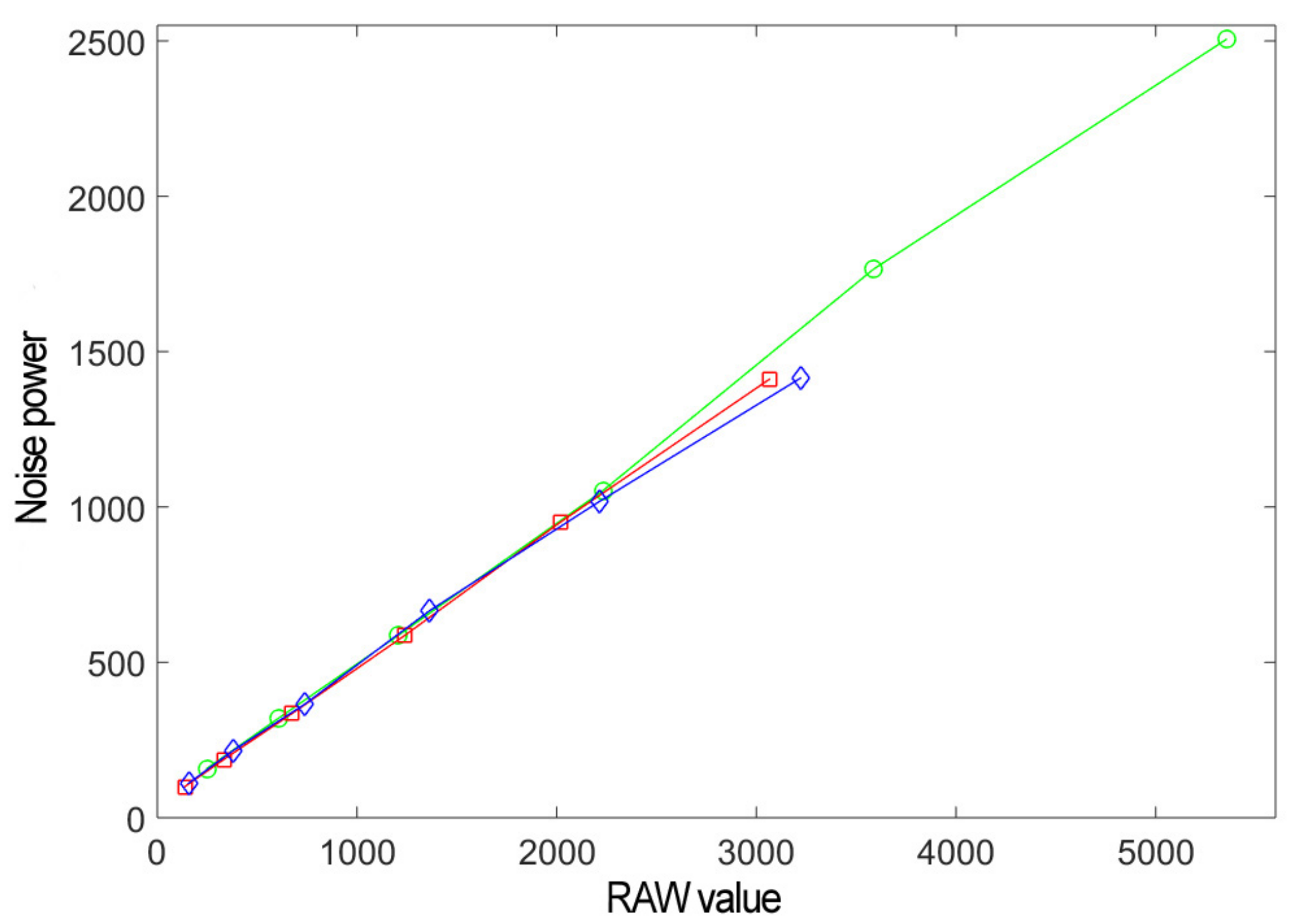
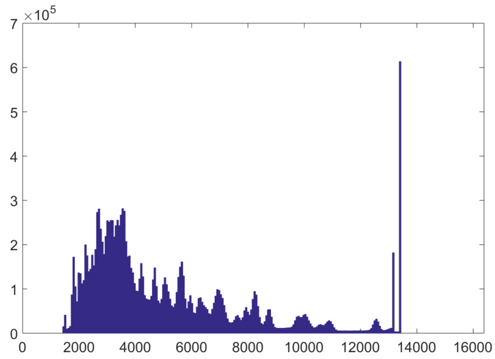
3.2. Experiment: Canon 50D Noise Model at ISO 100

To show an example, let us obtain the noise model of the Canon 50D camera at ISO 100. First, we measure the read noise as the standard deviation of a darkframe: it is $N_r=6.47$ DU. Then, we obtain the photon transfer curve (Equation (31)) to calculate the gain G at ISO 100. We use the six gray patches in the Colorchecker Classic chart to obtain the set of points $(S_i,N_i^2)$, $i=1,\dots ,K$. Since there are three channels and six patches per channel, we have $K=18$.

The blacklevel (1024 DU at ISO 100 for the Canon 50D) is subtracted from the RAW values and, then, the signal and square of the noise for each patch are calculated. We show the results in Figure 1.

We confirm the linearity of the three channels and that the green one is the most sensitive. For a detailed linearity analysis of an image sensor, see the work of Wang and Theuwissen [23], Wakashima et al. [24]; in addition, Wang et al. [25] presented a highly linear CMOS Image Sensor with a digitally assisted linearity calibration.

The least squares average straight line is:

$$N^2=G·S+N_r^2=0.447·S+44.5$$

(36)

The read noise of this camera fits the first model explained in Section 2.1. In the deepest shadows (small value of S), the square of the read noise dominates $44.5\gg 0.447·S$, whereas, in the highlights (large value of S), only photon noise is relevant, $0.447·S\gg 44.5$.

Reversing $G=0.447$, we obtain the so-called unit gain factor $k=2.2$; i.e., at ISO 100, the Canon 50D has a ratio of 2.2 photons per RAW unit DU. Another technical data associated to a pixel is its maximum value measured in electrons (full well capacity). Since it is a 14-bit camera (maximum RAW value $S=2^{14}-1=$ 16,383) and we know that the gain at ISO 100 is $k=2.2$ $e^{-}$/DU, the theoretical full well capacity is 16,383 · 2.2 = 36,043 $e^{-}$. Taking into account the blacklevel offset 1024, we have (16,383 − 1024) · 2.2 = 33,790 $e^{-}$. However, the value that saturates the Canon 50D is not the theoretical one but a smaller one. In Figure 2, we plot the histogram of a partially overexposed photo. The right-hand peak corresponds to the RAW value 13,433 DU, approximately 1/3 EV below the theoretical maximum 16,383 DU. Using this value, the full well capacity is (13,433 − 1024) · 2.2 = 27,300 $e^{-}$.

We can also use the tag called Whitelevel in the RAW metadata; in this case, it is 13,200 DU. The white level is the RAW value up to where the photon transfer curve is a straight line and the noise measurements are reliable. From this value, the calculated noise is underestimated because of saturation of the RAW value. Using Whitelevel, the result is (13,200 − 1024) · 2.2 = 26,785 $e^{-}$.

In practice, these small differences are not a problem for noise considerations, since the $SNR$ is always high enough in the highlights; the true problem is when the photographer tries to maximize the $SNR$ by exposing to the right and there is a risk that some channels are saturated without knowing it (first, the green channels). Unfortunately, cameras do not show the RAW histogram but the JPEG one when taking the photo, so there is risk of burning out the highlights. In our case, we use the value of 27,000 electrons, unless we indicate otherwise.

To know the full well capacity of a pixel is interesting, but it says little about a technology; a sensor with larger pixels and the same technology will have a higher full well capacity. Thus, the number of electrons per unit area is more informative. The Canon 50D carries an APS-C sensor (CMOS sensor of size 22.3 × 14.9 mm) of 4752 × 3168 pixels (15.1 Mp). Therefore, we have a pixel size (including the non-light gathering part) of $4752/22.3=3168/14.9=4.7$ $\mathsf{\mu }$m and a density of 27,000/4.7${}^2=1222$ $e^{-}/\mathsf{\mu }$m${}^2$ (electrons per micrometer squared).

4. Results

In this section, we show how the camera noise model is used to characterize the sensor noise performance. We show first the analysis of the Canon 50D in detail and next we compare different cameras to show how different technologies (noise models) behave. Thanks to the use of the photographic noise measurements, the obtained values are easily understandable for any photographer and we are sure that, when comparing different cameras, relevant factors such as pixel and sensor sizes or visual acuity are taken into account.

4.1. Canon 50D Analysis

As an example of a camera analysis, we complete the study of the Canon 50D obtaining the SNR curves at different ISOs. To see how low the read noise of the Canon50D is, we compare the results with the ideal SNR curves, i.e., if the read noise were zero. We provide a deep analysis of the results to emphasize the relationships between sensor technology (noise model) and photography parameters such as camera exposure settings.

4.1.1. Canon 50D: Signal to Noise Ratio Curves

We repeat the procedure explained in previous section to obtain the noise models at different ISOs. The results are:

$$\begin{array}{ccc}\hfill ISO100:N^2& =& 0.447·S+44.5\hfill \\ \hfill ISO200:N^2& =& 0.885·S+53.4\hfill \\ \hfill ISO400:N^2& =& 1.750·S+78.6\hfill \\ \hfill ISO800:N^2& =& 3.629·S+162.2\hfill \\ \hfill ISO1600:N^2& =& 7.074·S+420.2\hfill \\ \hfill ISO3200:N^2& =& 14.555·S+1667.1\hfill \end{array}$$

Theoretically, doubling the ISO doubles G, i.e., $G_{IS{O}_{2X}}=2·G_{IS{O}_X}$ (the same amount of photons doubles the RAW value). Empirical results are close to the theoretical values:

$$G/G_{IS{O}_{100}}=[1,1.9,3.9,8.1,15.8,32.5]\simeq [1,2,4,8,16,32]$$

(37)

For the read noise, the ISO dependency is not so simple since there is one part that depends on the ISO and another that does not. We analyze in depth this dependency below.

The $SNR$ in EVs scale is:

$$SN{R}_{EV}=S_{EV}-\frac{1}{2}{log}_2(G·2^{S_{EV}}+N_r^2)$$

(38)

Substituting the values of G and $N_r^2$ of Equation (37) into Equation (38), we obtain the SNR curves. The ideal sensor would be the one with zero read noise. The real (solid lines) and ideal (dashed lines) $SNR$ curves are plotted in Figure 3. Understanding Figure 3 is the key to understanding the relationship among exposure, “exposure”, noise and ISO for any sensor.

For small values of S (deep shadows), real $SNR$ curves are straight lines with +1 EV slope; for high signal values (highlights), slope is $1/2$ EV. In addition, we can see that all curves are parallel at highlights. The difference when changing ISO is not in the slopes, but in the y-intercept values (the SNR value for $S=0$ EV) and in the interval of S values where the slope of the SNR is 1 or $1/2$ (for which S value the line with slope 1 starts to bend).

For the same value of S, the higher is the ISO, the higher is the gain and therefore the fewer are the photons required to obtain the same RAW value, thus the exposure is lower and, accordingly, the $SNR$ is worse; i.e., the $SNR$ is reduced when raising the ISO.

For the highlights, where the signal-to-noise ratio is maximal and can be approximated by $SN{R}_{EV}=\frac{1}{2}{S}_{EV}-\frac{1}{2}{log}_{2}G$, the curves are parallel straight lines (all slopes $1/2$), with 0.5 EV distance between ISO X and ISO 2X curves; e.g., from ISO 100 to ISO 200, $\frac{1}{2}{log}_2(G_{IS{O}_{200}}/G_{IS{O}_{100}})=1/2$. The difference between $SNR$ values in the highlights between cameras is due to the different unit gain values: the higher is the k factor (the lower is the G), the higher is the $SNR$, since a large unit gain means a higher full well capacity. In the shadows, due to the dominant read noise, although the lines are parallel (all of slope 1), the difference between curves is not constant as happens in the highlights.

If a large value of full well capacity is a guarantee of a better $SNR$ in the highlights, a small read noise is a guarantee of a better $SNR$ in the shadows. A large value of unit gain implies a greater number of electrons per RAW unit, so the region where photon noise is the dominant one is reach faster.

In the ideal case, the curves are straight lines with a $1/2$ slope for any signal value S. The smaller is the distance from the real SNR to the theoretical maximum SNR value, the better is the sensor. In Figure 3, we observe that the real curves are separated very quickly from the ideal curves and that, for the deep shadows zone, the Canon 50D has $SNR$ values well below the theoretical limits (around 3 or 4 f-stops depending on the ISO). For example, the SNR curve for ISO 100 only fits the ideal curve for the highlights, starting around $S\simeq 11$ EV. That means that a sensor with a smaller read noise would improve the $SNR$ at almost any exposure value. It also tells us that, if we do not expose to the right, we would obtain a noisier image than we could otherwise.

For example, let us suppose we are photographing a dark scene (a black cat on a coal pile at night) at ISO 100 and we want the maximum brightness value to be $S=6$ EV. We set the exposure on the camera to get the correct exposure in the photo. In that case, we obtain $SNR=2.8$ EV (see the black line in Figure 3 for ISO 100 when $S=6$ EV). For darker areas than $S=4$ EV, the $SNR$ falls approximately at a rate of 1 EV per stop. Now, let us take another photo exposing to the right (there is no space on the right side of the RAW histogram). It means we have overexposed 8 stops in this second photo. When we see this photo on the computer, it looks like a white cat in the snow on a very sunny day. We correct the brightness of the photo with the computer underexposing the 8 extra stops so we have the final correct photo (to correct the “exposure” with the computer does not change the $SNR$). Both photos have the same final brightness, but they look very different. In the second photo, $SNR=7.58$ EV (value for $S=14$ EV in the curve for ISO 100 in Figure 3), a SNR 5 EV better than the first one. In the first photo, you see a noisy cat, while in the second one, it is a clean cat. The difference is even greater in the darkest pixels of the photo. For example, for the first photo, $SNR=1$ EV for $S=4$ EV (a lot of noise), while $SNR=6.58$ EV in the second photo (no visible noise). It means that, in the case you want to recover the shadows, you will have no problem in the second photo since SNR is large enough.

4.1.2. Canon 50D: $SNR$, Exposure and ISO

Doubling the ISO multiplies by two the RAW value, the “exposure” signal S. Thus, the RAW value S EV for a given ISO has the same exposure as the value $S+1$ EV for double ISO. For example, $S=2$ EV for ISO 100 has the same exposure as $S=3$ EV for ISO 200. This way, we can check in Figure 3 the ISO and exposure relationship. Figure 4 shows the $SNR$ curves for small S values (for clarity, we omit the ISO 400 curve).

For the ISO 100 curve (black line), $SNR=-0.76$ EV for pixels with signal $S=2$ EV ($S=4$ DU). If we repeat the photo with the same exposure settings (shutter speed and f-stop) but ISO 200, the corresponding point is $S=3$ EV, $SNR=0.04$ EV on the red line (ISO 200). The improvement is very remarkable, 0.8 EV, close to the theoretical 1 EV increase when exposure, not “exposure”, is doubled (note that black and red curves in Figure 4 are very similar). In the case of the ISO 800 curve (blue line), the point $S=4$ EV has the same exposure as $S=2$ EV for ISO 200. For ISO 200, $SNR=-0.91$ EV for $S=2$ EV. For ISO 800, $SNR=0.10$ for $S=4$ EV. In this case, the improvement is still greater. However, it is smaller than the improvement we would achieve if instead of raising the ISO two EV we increase the exposure by two EV (note that the distance between the blue and red curve for the same value of S is larger). Repeating the analysis for the ISO 800, 1600 and 3200 curves, we obtain $SNR=-1.73$ EV for $S=2$ EV (ISO 800 blue line), $SNR=-1.44$ EV for $S=3$ EV (ISO 1600 magenta line) and $SNR=-1.44$ EV for $S=4$ EV (ISO 3200 cyan line). That is, to raise ISO beyond ISO 800 keeping constant the exposure hardly improves the $SNR$, and nothing at all above ISO 1600; the Canon 50D becomes ISO invariant at ISO 1600 approximately.

To analyze the influence of exposure keeping ISO constant, look at the $SNR$ values in Figure 4 for the same ISO. For example, moving from $S=2$ EV to $S=3$ EV for ISO 200, SNR improves from $SNR=-0.91$ to $SNR=0.04$, confirming that the $SNR$ grows linearly with the exposure (a +1 EV exposure implies a +1 EV in the $SNR$). For the case of ISO 800, we have the points $S=2,SNR=-1.73$ EV and $S=4,SNR=0.10$ EV. The improvement is 1.83 EV, close to the theoretical 2 EV.

In summary, in the shadows, the Canon 50D pixel $SNR$ grows linearly with exposure for any ISO, and also grows if the exposure is constant and you increase ISO, especially for low ISOs; for example, from ISO 100 to ISO 200. However, there is an ISO where the $SNR$ stagnates and has no advantage continuing to raise the ISO; the only way to keep improving the $SNR$ is by increasing exposure.

We repeat the analysis for the highlights in Figure 5.

The photon noise is the dominant noise in the highlights. The $SNR$ curves become straight lines with slope $1/2$. For a given RAW value S, the lower is the ISO, the better is the $SNR$, since the exposure s is greater and we know that $SNR\simeq \sqrt{s}$.

For example, let us consider $S=10$, $SNR=5.52$ for ISO 100 (black line in Figure 5). If the exposure is increased by 1 EV, we have $SNR=6.04$ (around $1/2$ EV more as predicted by theory). It is the same for the other ISO curves; e.g., for the ISO 800 curve (blue line), $S=10,SNR=4.05$ and $S=13,SNR=5.57$, a theoretical +1.5 EV improvement. If we maintain the exposure and raise the ISO, the $SNR$ must remain constant, since $SNR\simeq \sqrt{s}$. The values obtained for ISO 200 and 800 are $S=11$ and $SNR=5.55$ (red curve, ISO 200) and $S=13$ and $SNR=5.57$ (blue curve, ISO 800). Figure 5 also shows the case when raising the ISO while keeping the exposure constant does not affect the $SNR$: $S=10,SNR=4.0$ (ISO 800 blue line), $S=11,SNR=4.0$ (ISO 1600 magenta line) and $S=12,SNR=4.0$ (ISO 3200 cyan line).

In summary, to raise the ISO does not improve the SNR in the highlights, increasing the risk of clipping the highlights, since the same exposure produces a higher “exposure” and the RAW histogram is moved to the right side (1 EV every time ISO is doubled). For example, for the Canon 50D at ISO 100, the well capacity is 27,000 electrons; at ISO 200, it is half, 13,500 electrons, and so on.

Finally, the difference in the $SNR$ when we raise the ISO for the same value of S in the highlights is given by $\frac{1}{2}{log}_2(G_2/G_1)$. Every time ISO is doubled, $SNR$ loses 0.5 EV, since the same “exposure” value with double ISO is equivalent to halving the exposure, so $SNR=\sqrt{s/2}$, i.e., the $SNR$ is reduced $\sqrt{2}=1/2$ EV. We show this case in Figure 5 for $S=11$ and ISO 100, 200 and 1600. The values are: $SNR=6.0$ (ISO 100), $SNR=5.5$ (ISO 200) and $SNR=4.0$ (ISO 1600).

4.1.3. Canon 50D: Read Noise Model and Exposure

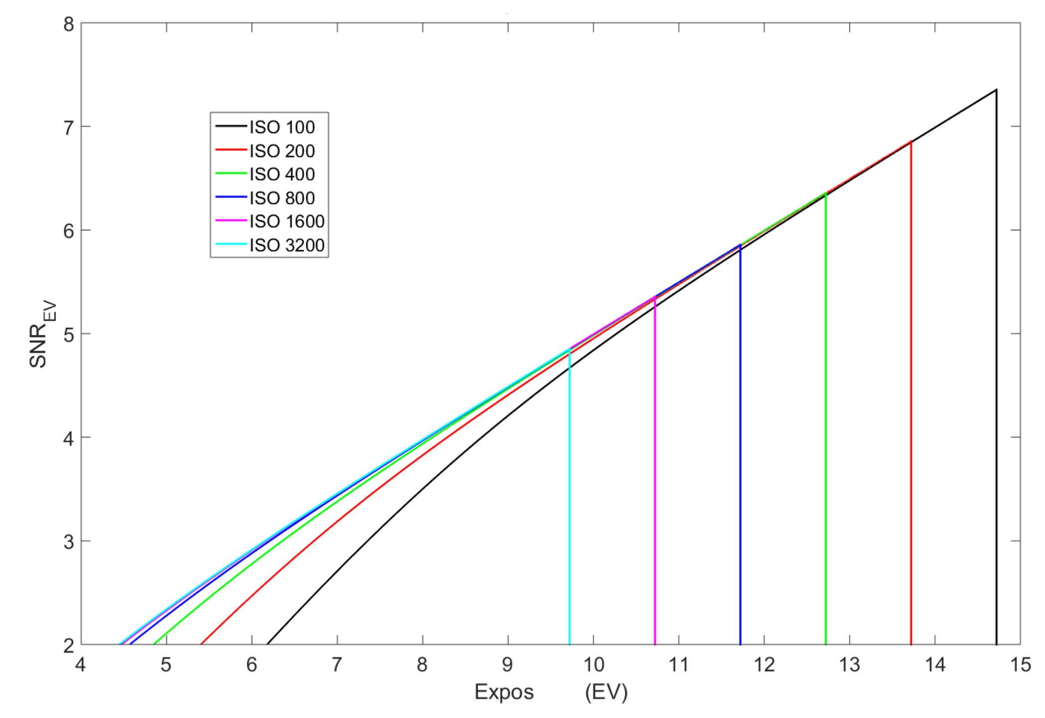
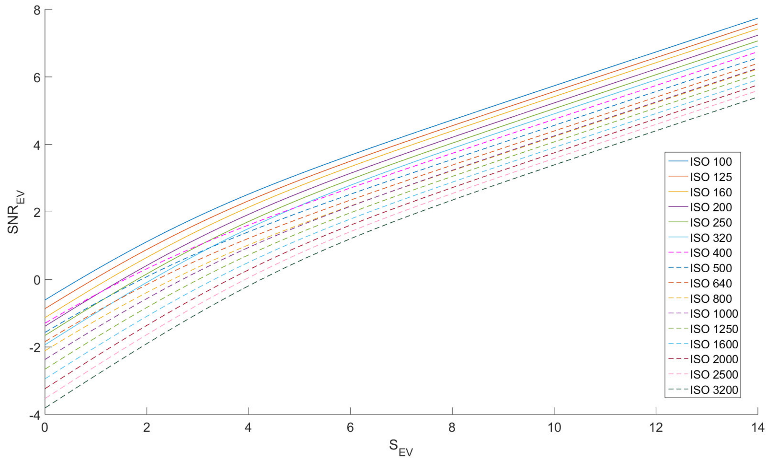
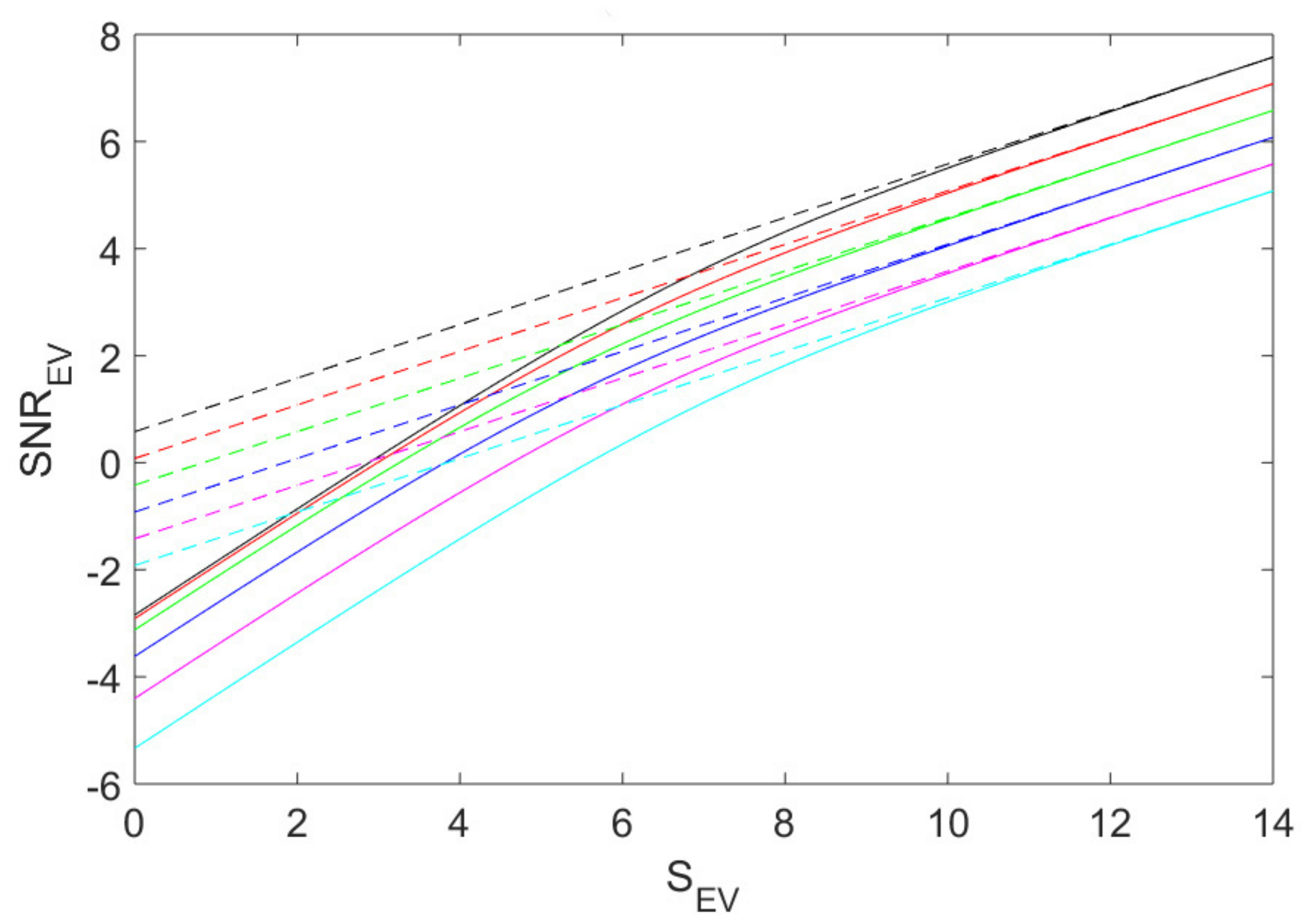
In previous sections we have analyzed the $SNR$ curves in the “exposure” or brightness domain. The Canon 50D read noise follows the Equation (2) model. The square of the total noise is $N^2=N_p^2+N_{r1}^2+N_{r2}^2=G^2·s+{(G·n_{r1})}^2+N_{r2}^2$. The read noise components are estimated using least squares [13]; at ISO 100, they are $n_{r1}=7.63$ and $N_{r2}=49.56$. Expressing G in terms of ISO and after some math, the resulting $SNR$ is:

$$SNR=\frac{s}{\sqrt{s+7.63+\frac{247.5}{{(ISO/100)}^2}}}$$

(39)

The $SNR$ in Equation (39) is very intuitive and easier to understand for a photographer since it is expressed in terms that he is familiar with, the exposure s (shutter speed and aperture) and ISO, rather than the $SNR$ expression in Equation (4) where camera settings are masked. It allows explaining in an understandable way to a photographer not familiar with math how to adjust camera settings in order to obtain the cleanest image possible (the best $SNR$ according to his photographic restrictions and requirements).

In Equation (39), it is clear that the best way to increase the $SNR$ is to increase s (more light equals to less visible noise), since, while the numerator grows at a rate of s, the denominator does at a rate less than $\sqrt{s}$. The saturation exposure is the limit (expose to the right, i.e., no gaps on the right side of the RAW histogram without clipping). The full well capacity for the 50D is around 27,000 $e^{-}$ at ISO 100 (at double the ISO, half as much light s is needed for the same RAW value S).

We have three noise sources: the photon noise $\sqrt{s}$ that increases with the exposure, the constant pre-amplifier read noise $n_{r1}=2.76$ $e^{-}$ and the post-amplifier read noise that depends on the ISO $n_{r2}=15.73/(ISO/100)$ $e^{-}$ (worst case for ISO 100). For the highlights, only photon noise is relevant. For example, for ISO 100, the total squared read noise is $n_r^2=255.13\ll s$ (s can take values up to 27,000). If ISO is raised, $\sqrt{s}$ and the $SNR$ are reduced since the maximum value of s decreases. The advantage of raising the ISO is in the deep shadows. The minimum noise value (ISO 100) is $n_r=\sqrt{7.63+247.5}=15.97$ $e^{-}$ $\simeq n_{r2}$. When ISO is raised, the input referred minimum value reduces. For example, at ISO 3200, $n_r=\sqrt{7.63+247.5/{\left(32\right)}^2}=2.80$ $e^{-}$ $\simeq n_{r1}$.

The $SNR$ curves for the Canon 50D as a function of exposure are given in Figure 6 (binary log-log scales; vertical lines correspond to the maximum exposure value for each ISO).

This figure is the most intuitive demonstration of the expose to the right rule in digital photography: $SNR$ is a monotonically increasing function of exposure. The highest value of $SNR$ is obtained for the maximum exposure value (black vertical line). It also demonstrates graphically the “expose” to the right rule for this camera: given an exposure value s, the highest ISO has the best $SNR$ in the shadows. The price to be paid for this improvement is in the highlights: vertical lines move to the left 1 EV every time the ISO is doubled (dynamic range is reduced 1 EV in the highlights). “Exposure” to the right difference is remarkable for low ISOs (see the large distance between the red and black curves for ISO 100 and 200 for small s values). However, it makes no difference at high ISOs (the magenta (ISO 1600) and cyan (ISO 3200) lines are overlapped). Thus, once the camera becomes ISO invariant, there is no reason to raise ISO, since it reduces the dynamic range with no shadows $SNR$ improvement.

Given a scene dynamic range, photographer can adjust the exposure settings using the info in Figure 6 and his artistic restrictions, e.g., to preserve the details in the shadows or not to burn out the white wedding dress details. For example, if photographing a sunset landscape with a high dynamic range, shoot at ISO 100. You will get the highest dynamic range of the sensor (if it is lower than the scene, you will have to take several photos, High Dynamic Range Photography HDR), but in the darkest areas you will get garbage (note that the zones of the scene that have an exposure of $s=4$ EV, ten stops less than the saturation value, will have a $SNR=0$ EV, i.e., visible noise for sure when lifting the shadows with the computer). If it is a low dynamic range scene, raise the ISO. Just from ISO 100 to ISO 200, the $SNR$ is improved +1 EV for many exposure values. From ISO 400, the gain is reduced and, from 800 to 1600, it becomes negligible.

4.2. $SNR$ and ISO for Dual Gain ISO Invariant Sensors

For a dual gain sensor, the $SNR$ curves are more complicated. In Figure 7 we have the Nikon D500 $SNR$ curves for ISOs between 100 and 3200 (solid lines low gain ISOs; dashed lines high gain ISOs). Notice that some curves intersect.

For medium-high signal levels, photon noise dominates, thus it does not matter what kind of sensor camera has. Whatever the ISO, all curves grow at a $\sqrt{s}$ rate and the lower is the ISO, the better is the $SNR$ for the same RAW value. The difference is in the low levels (shadows). Note that the $SNR$ is better at ISO 400 than at some lower ISOs.

For a non dual gain sensor such as in the Canon 50D, the $SNR$ doubles in the shadows when the exposure doubles. However, in a dual gain sensor, this behavior is only valid for the low gain mode (low ISOs). For high ISOs, the signal is already pre-amplified, thus receiving less amplification in the second gain stage. The overall effect is that a lower read noise is achieved in the deep shadows, but at the cost that the $SNR$ does not improve so fast with signal. That explains why the SNR curves in the shadow zone for ISO 400 or higher are not parallel to the ISO 320 or lower curves. For high signal values, all of them are parallel, because only photon noise is relevant.

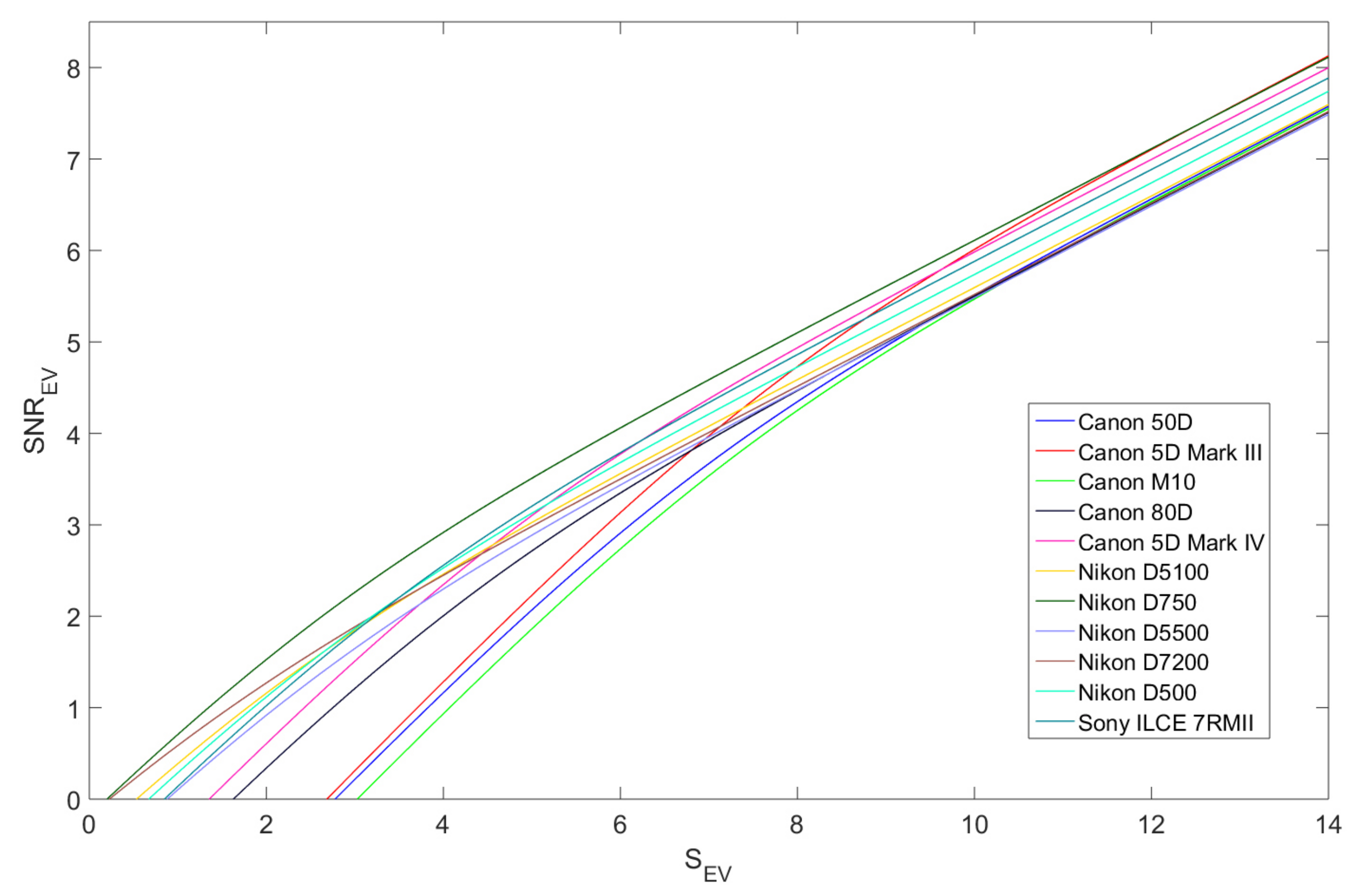
4.3. Comparative Performance Evaluation

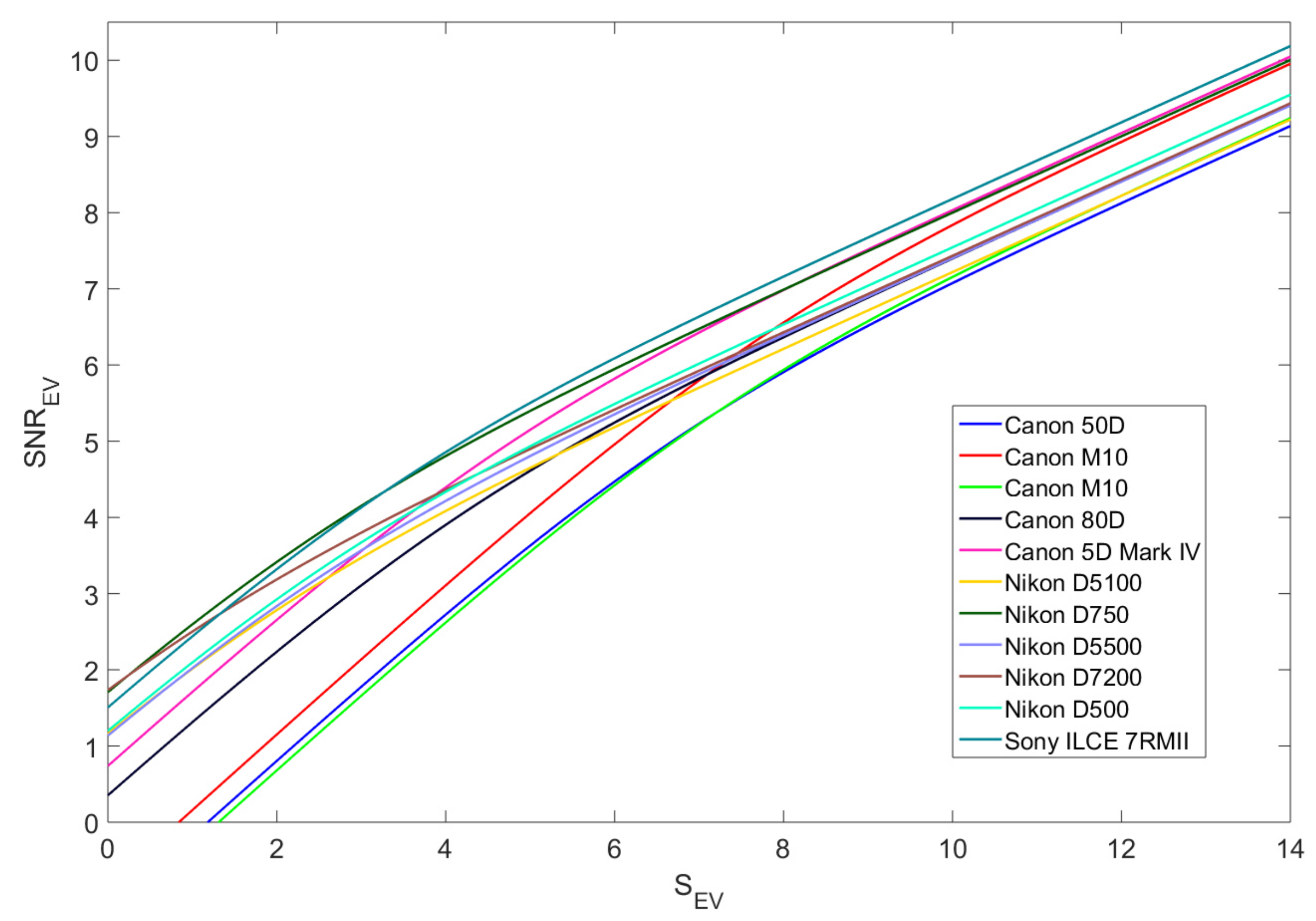
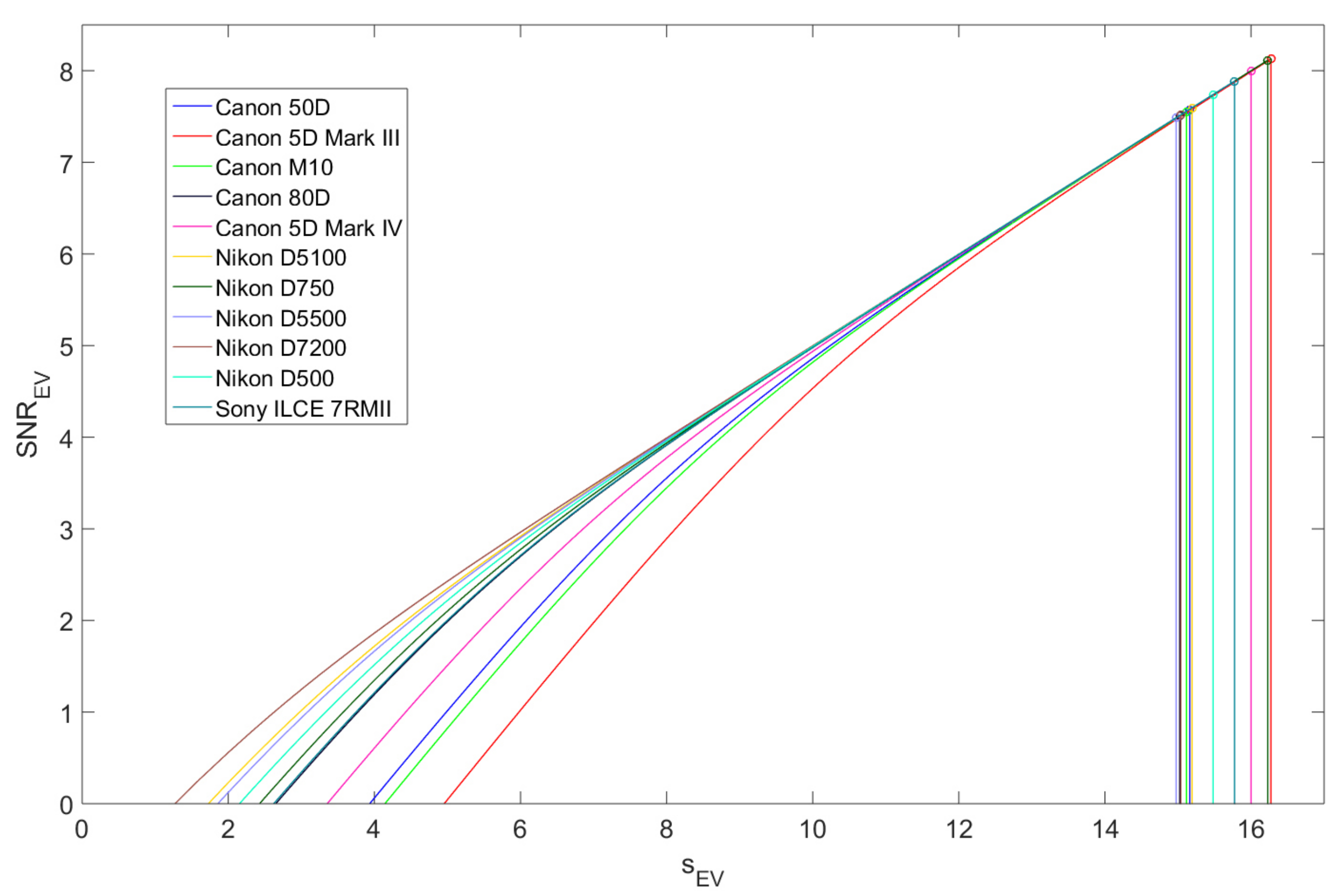
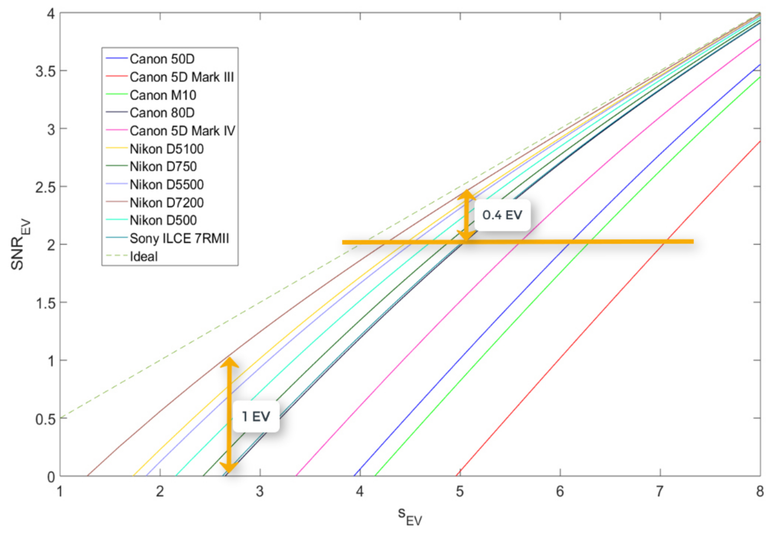
We analyzed different cameras in order to compare different technologies and verify how recent CMOS image sensors advances are transferred to real world cameras.

Table 1. Cameras analyzed and basic data.

Camera	Dimensions	Mp	Pixel Size	k
Canon 50D	$22.3\times 14.9$	15.1	4.7	2.23
Canon 5DMIII	$36\times 24$	22.3	6.3	4.83
Canon M10	$22.3\times 14.9$	18	4.3	2.17
Canon 80D	$22.3\times 14.9$	24	3.7	2.03
Canon 5DMIV	$36\times 24$	30.1	5.4	4.00
Nikon D5100	$23.6\times 15.6$	16.2	4.8	2.29
Nikon D750	$35.9\times 24$	24	6	4.69
Nikon D5500	$23.5\times 15.6$	24.2	3.9	1.97
Nikon D7200	$23.5\times 15.6$	24	3.9	2.05
Nikon D500	$23.5\times 15.7$	20.9	4.2	2.79
Sony 7RMII	$35.9\times 24$	42	4.5	3.42
Fuji XT-2	$23.6\times 15.6$	24	3.9	1.69

contains the list of cameras analyzed and basic data (k is the inverse of gain, i.e., electrons per unit RAW ($e^{-}/DU$) for base ISO).

4.3.1. Pixel $SNR$ Curves

We show in Figure 8 and Figure 9 the $SNR$ curves vs. “exposure” and exposure at ISO 100, respectively.

$SNR$ curves can be divided in three different signal sections: (i) where the read noise is the most important noise source (very small signal values); (ii) where photon noise starts to be relevant in the total noise (small signal values, depending on the particular camera read noise model); and (iii) where the photon noise limit is reached out (camera differences depend on G value).

In the highlights, where $SNR\simeq \frac{1}{\sqrt{G}}·\sqrt{S}=\sqrt{s}$, all lines are parallel ($1/2$ EV slope). The difference in Figure 8 is due to the $-\frac{1}{2}{log}_{2}G$ factor. It translates to a different well capacity in the normalized version in Figure 9. The smaller is the G value, the better is the $SNR$. In other words, the camera that needs more electrons per DU (greater value of k, see Table 1) has a greater full well capacity, and therefore will achieve a better $SNR$ in the highlights. A higher maximum $SNR$ value is not the reason because a large k is better; in the end, it does not matter if $SNR=7$ or 8 EV, since both photos look clean. The real reason a large k value is better is because it allows that the $SNR$ grows faster out of the photon noise region (compare the slopes for the different cameras at low signal values in both figures). However, even though some full frame cameras benefit from a larger pixel area, depending on the read noise value, this factor is relevant or not. For example, the Canon 5D MIII (red curves) has a large k (large well capacity and $SNR$ grows more quickly) but it is strongly penalized by a large read noise, resulting in a general poor pixel noise performance in comparison with other cameras at ISO 100.

Of course, since technology improves, the read noise is continuously being reduced and newer cameras show a performance close to the ideal photon noise regime (a $1/2$ EV straight line) even at very small signal values. In Figure 10, we show the model $SNR$ (solid lines) vs. the ideal $SNR$ (zero read noise) (dashed lines) for each camera.

An interesting pixel comparison in Figure 10 is between the Nikon D750 (dark green line) and D7200 (brown line). They have practically the same read noise at ISO 100, $N_r\simeq 1$ DU. However, the D750 pixel area is ${(6/4.9)}^2=1.5$ times greater than D7200. Assuming that both cameras have the same technology, that 50% extra surface means more electrons per RAW unit (check Table 1 for k for each camera; it is more than double for the D750). Although they have the same read noise, the D750 is better since the $SNR$ grows quickly and its full well capacity is larger. This fact generates many confusions when analyzing or comparing sensors in the photographer community. The fact that a pixel in two photos taken with the same exposure camera settings, one with the D750 and the other one with the D7200, looks equally bright in both photos (same “exposure” or RAW value) does not mean that the two pixels capture the same amount of photons. The D750 has more electrons, and therefore has a better $SNR$. An example of this confusion is the calculation of the pixel dynamic range. If we set the read noise as the minimum signal value, both cameras will have the same dynamic range, since they have the same read noise in RAW units. However, if we set the minimum signal level at $SNR=2$ EV, they no longer have the same dynamic range, since in Figure 10 it is clear that the D750 reaches the $SNR=2$ EV value before the D7200, i.e., $R{D}_2\left(D750\right)>R{D}_2\left(D7200\right)$. The cause is the greater sensitivity of the D750 pixel. That is why the $SNR$ curves are the important ones. Data such as the dynamic range are useful because they condense a lot of information into a single parameter, but sometimes they hide relevant information and can produce misunderstandings if it is not clear how it is calculated (the minimum signal definition).

The analysis can be also carried out in the electrons domain. To quantify the performance difference between pixels from different cameras at low charge values, set a signal level on the horizontal axis and measure the difference in the vertical axis between the cameras you want to compare. For example, in Figure 11, we compare the Canon 80D and the Nikon D7200 for both $SNR=0$ EV and $SNR=2$ EV. Note that the difference is reduced (from 1 EV to 0.4 EV) when minimum $SNR$ required is more demanding (from $SNR=0$ EV to $SNR=2$ EV).

We repeated the analysis at ISO 100 for the other ISOs. In Figure 12, we show the results obtained for ISO 200 (Fuji XT-2 appears for the first time since its base ISO is 200) and ISO 3200.

A self explanatory example about technology improvement is shown in Figure 12: the Canon 5D Mark III full frame pixel has worse $SNR$ in the shadows than many APS-C format cameras in the figure, including its four-year newer model the Canon 80D, despite having a larger pixel. However, at ISO 3200, the Canon 5D Mark III imposes its largest sensor size over all APS-C cameras in the figure. This is because, at high ISOs, the contribution of the post amplifier read noise is negligible and the important factor is the amount of light that pixel gathers, i.e., pixel size.

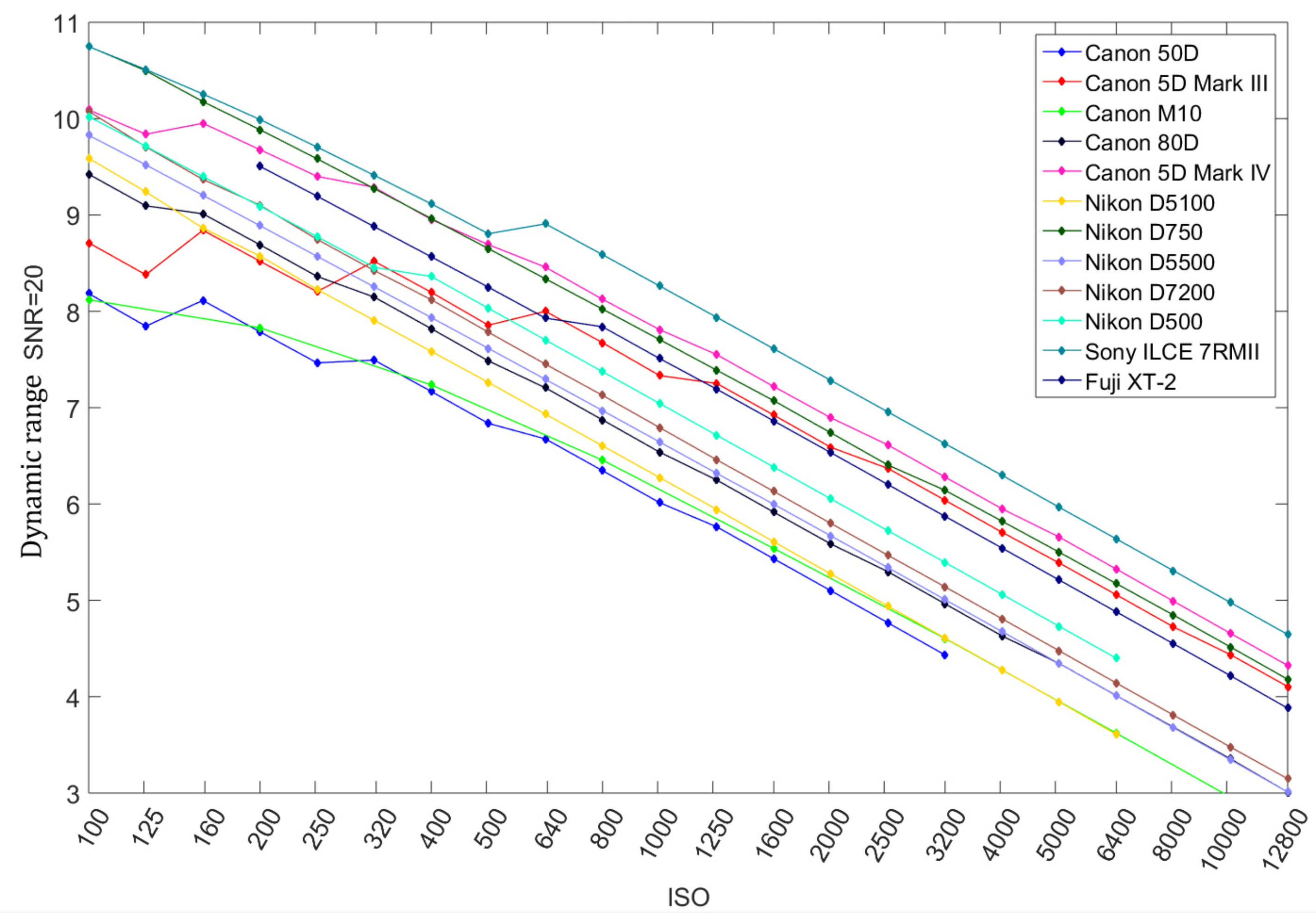
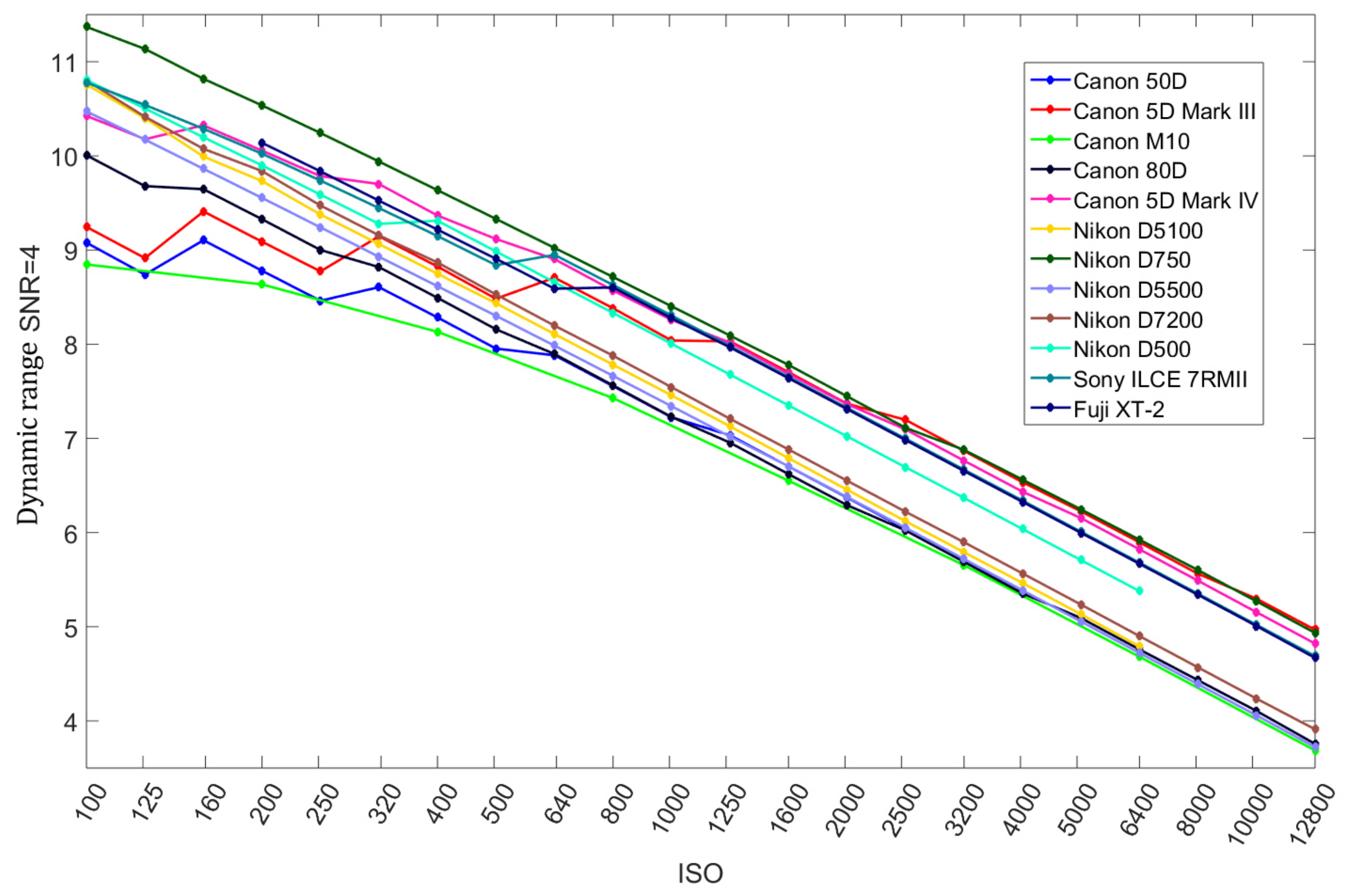
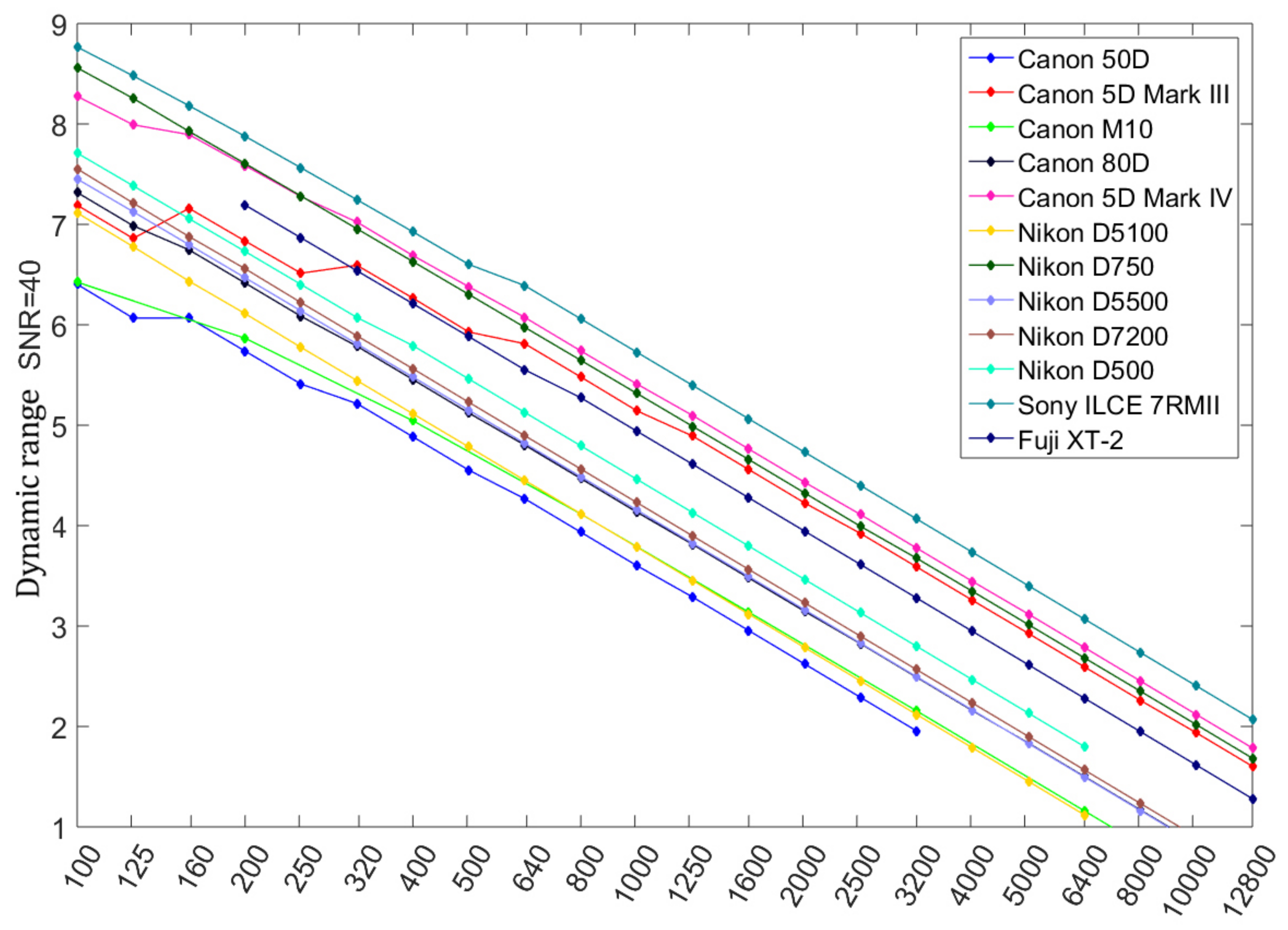
4.3.2. Pixel Dynamic Range

When the minimum signal is defined at $SNR=1=0$ EV (see Equation (14)), we have:

$$S_{mi{n}_0}=\frac{G+\sqrt{G^2+4·N_l^2}}{2}$$

(40)

The dynamic range for $SNR=0$ EV is:

$$R{D}_0=14-{log}_2{S}_{mi{n}_0}$$

(41)

Figure 13 shows $R{D}_0$ for each camera and ISO.

An important precaution when comparing $SNR$ curves at the same ISO and dynamic range values is to check if all cameras use the same ISO scale. The standards where the ISO scales are defined are beyond the scope of this paper, but, just by taking the same photo and comparing the shutter speed and f-number suggested by camera autoexposure system for a given ISO, we can test that the ISO scale is similar. All of these cameras obtained a similar exposure setting but the Fuji camera, with an approximately $0.5$ EV difference. In other words, when using ISO 200, the Fuji pixel receives a higher exposure, obtaining a better noise performance since more light is arriving. This was expected as the ISO scale for the Fuji camera starts at ISO 200 instead of more common ISO 100. This is the reason the dynamic range values for Fuji XT-2 in Figure 13 are much better than other APS-C format similar cameras.

In the case that the minimum acceptable $SNR$ is $SNR=4=2$ EV (a more demanding situation, e.g., if photo is being printed at a larger size or if the photographer’s criterion is more restrictive), we have:

$$S_{mi{n}_2}=8·G+4·\sqrt{4·G^2+N_l^2}$$

(42)

and its corresponding dynamic range definition:

$$R{D}_2=14-{log}_2{S}_{mi{n}_2}$$

(43)

In Figure 14, we show $R{D}_0$.

Figure 13 and Figure 14 results vary for two reasons. On the one hand, since $SNR=2$ EV is a more demanding criterion, dynamic ranges decrease in Figure 14. On the other hand, they do not decrease by the same amount for all cameras. Cameras that have a large k factor (the $SNR$ grows more quickly), the dynamic range is kept higher than cameras with a small k factor.

4.3.3. Photo Level Results

In this section, we obtain the definitive comparison, normalizing pixel results to a common scale where pixel and format size effects are taken into account. The photographic $SNR$ functions are obtained from the pixel $SNR$ using Equation (26).

In Figure 15, we show the results at ISO 100 when the circle of confusion is 25 $\mathsf{\mu }$m, and, in Figure 16, for ISO 200 and 3200. The original Fuji curves have been modified to take into account its different ISO scale.

In the highlights, the full frame cameras are approximately 2/3 EV better than APS-C, as theory predicts due to different sensor sizes. In the read noise domain (low signal values), some APS-C cameras outperform some full frame camera, such as the old Canon 5D MIII. It is in the deepest shadows where a very low read noise really matters. Of course, the full frame ability to gather more light allows the $SNR$ to grow more quickly than the APS-C, but, while the read noise is the dominant one, the difference is very small. Although comparing absolute $SNR$ values is the way we compare the noise performance of different cameras, it is important to point out that a better $SNR$ is only useful if the $SNR$ value is above the established minimum noise quality requirements. It becomes irrelevant if it is higher than the $SNR$ where noise is not visible at all.

The photographic dynamic range for all cameras is obtained using a full frame circle of confusion of 25 $\mathsf{\mu }$m and $SN{R}_{photo}=20$ (see Equations (28) and (30)). In Figure 17, we show the results (in this case, no ISO normalization has been applied to the Fuji XT-2 in order to preserve its nominal ISO).

Alternatively, the photographic dynamic range can be obtained graphically from the $SNR$ curves: draw a horizontal line in the $SNR$ curves at the desired $SN{R}_{photo}$ value; the minimum signal value for each camera is the value where that line and the corresponding $SNR$ curve are intersected.

The more demanding are the sharpness and noise criteria (smaller circle of confusion and larger $SN{R}_{photo}$), the lower is the dynamic range. In Figure 18, we have the results when the full frame circle of confusion is reduced to $C=20$ $\mathsf{\mu }$m and the $SNR$ is increased to $SNR=40$. The new dynamic range is lower than in Figure 17 and high gain mode benefits in dual gain sensors almost vanishes.

5. Discussion and Conclusions: How to Expose in Digital Photography

We have shown how the noise analysis of a pixel in any image sensor can be translated to interesting noise measures in photography. In particular, we have explained how to calculate the scene dynamic range that a camera is able to capture in a single photo with an acceptable noise quality (the photographic dynamic range). We have seen that there is not a unique value, since it depends on the amount of noise that a viewer can tolerate in a photo, i.e., what he understands as acceptable in noise terms. We have shown how to quantify this subjective criterion through the minimum $SNR$ value (higher for very demanding observers or observation conditions) and how to normalize different sensor sizes with the circle of confusion value (higher for larger image formats).

We have seen how different available technologies are responsible of different $SNR$ curves patterns. However, all of them are benefited when the light gathered is increased. Therefore, the expose to the right technique, where the RAW histogram is moved to the right as far as possible before saturating the pixel, is the best a photographer can do to obtain the cleanest image. However, we have seen that this technique can have some practical problems and restrictions, such as aesthetics requirements (risk of blur and depth of field required).

In cameras where the downstream noise is relevant, when exposure cannot be increased and there are gaps on the right side of the histogram, the best is to “expose” to the right by raising the ISO until before clipping the highlights and before the pre-amplifier read noise becomes the dominant read noise term. If downstream read noise is negligible not only at high ISOs but at all ISOs, “expose” to the right makes no sense since $SNR$ is not affected by ISO and we can adjust brightness in camera or in computer with no big difference.

However, in many cameras today, where the sensor has two gain modes and read noise is drastically reduced at some intermediate ISO, the optimal camera exposure settings becomes more complicated and the ISO that maximizes the $SNR$ must be obtained from the $SNR$ curves depending on the scene dynamic range. If the dual gain sensor is also ISO invariant for each ISO interval, as is usual, the decision is reduced to knowing which gain mode must be selected. For example, if gain mode is changed at ISO 400, the photographer must decide whether to use ISO 100 (low gain mode) or ISO 400 (high gain mode). If it is a high dynamic range scene, use ISO 100; if not, ISO 400 is a better option if highlights are not burned out.

No matter the technology, in photon noise regime, all cameras have the same behavior. To achieve this ideal limit as quickly as possible, the largest number of electrons per DU as possible is best. This is the main advantage of a bigger sensor format. However, this goal is opposed to the demands of higher resolution sensors (smaller pixels). Therefore, manufacturers must improve technology before a new camera is released on the market to guarantee that pixel noise performance is similar (by increasing the quantum efficiency, microlenses, stacked and backilluminated designs, and manufacturing) while photographic $SNR$ performance is usually improved. Overall, 24 Mp seems the standard resolution for today’s consumer cameras in the mid price range, with higher resolution models that benefit from image sensors technology developments for phone cameras. In the future, ILC camera makers should be more focused in improving the processing abilities and camera functionalities since phone cameras are minimizing their intrinsic unsolvable physical limitation (a much smaller sensor) in very clever ways, specially thanks to computational photography techniques.

References

1. Camera Imaging Products Association: Digital Cameras Report. Available online: http://cipa.jp/stats/dc_e.html (accessed on 1 September 2019).
2. Gye, L. Picture This: the Impact of Mobile Camera Phones on Personal Photographic Practices. Continuum 2007, 21, 279–288. [Google Scholar] [CrossRef]
3. Fontaine, R. The state of the art of smartphone imagers. In Proceedings of the International Image Sensor Conference, Snowbird, UT, USA, 23–27 June 2019; p. R6. Available online: https://www.imagesensors.org/PastWorkshops/2019Workshop/2019Papers/R01.pdf (accessed on 10 September 2019).
4. Bhandari, A.; Raskar, R. Signal Processing for Time-of-Flight Imaging Sensors: An introduction to inverse problems in computational 3-D imaging. IEEE Signal Process. Mag. 2016, 33, 45–58. [Google Scholar] [CrossRef]
5. Wang, J.; Zhang, C.; Hao, P. New color filter arrays of high light sensitivity and high demosaicking performance. In Proceedings of the 2011 18th IEEE International Conference on Image Processing, Brussels, Belgium, 11–14 September 2011; pp. 3153–3156. [Google Scholar] [CrossRef]
6. Chan, C.C.; Chen, H.H. Improving the Reliability of Phase Detection Autofocus. Electron. Imaging 2018, 2018, 241-1–241-5. [Google Scholar] [CrossRef]
7. Kirkpatrick, K. The edge of Computational Photography. Commun. ACM 2019, 62, 14–16. [Google Scholar] [CrossRef]
8. Koppal, S.J. A Survey of Computational Photography in the Small: Creating intelligent cameras for the next wave of miniature devices. IEEE Signal Process. Mag. 2016, 33, 16–22. [Google Scholar] [CrossRef]
9. Knowledge Sourcing Intelligence LLP. CMOS Image Sensor Market: Forecasts from 2019 to 2024. Technical Report. May 2019. Available online: https://www.knowledge-sourcing.com/report/cmos-Image-sensor-market (accessed on 5 September 2019).
10. Photonstophotos.net. Available online: http://photonstophotos.net (accessed on 3 September 2019).
11. Dxomark. Available online: http://dxomark.com (accessed on 3 September 2019).
12. Boukhayma, A.; Peizerat, A.; Enz, C. Temporal Readout Noise Analysis and Reduction Techniques for Low-Light CMOS Image Sensors. IEEE Trans. Electron Devices 2016, 63, 72–78. [Google Scholar] [CrossRef]
13. Igual, J. Noise in CMOS Image Sensors: A Photographic Analysis of Noise Models in Consumer Cameras. Sensors 2019. submitted. [Google Scholar]
14. Vargas-Sierra, S.; Liñán-Cembrano, G.; Rodríguez-Vázquez, Á. A 151 dB High Dynamic Range CMOS Image Sensor Chip Architecture With Tone Mapping Compression Embedded In-Pixel. IEEE Sens. J. 2015, 15, 180–195. [Google Scholar] [CrossRef]
15. Photography—Electronic Still-Picture Imaging—Noise Measurements; International Organization for Standardization: Geneva, Switzerland, 2017.
16. Photography—Digital Still Cameras—Determination of Exposure Index, ISO Speed Ratings, Standard Output Sensitivity, and Recommended Exposure Index; International Organization for Standardization: Geneva, Switzerland, 2019.
17. Baer, R. ISO Sensitivity. In Proceedings of the IEEE 2005 ISSCC Circuit Design Forum: Characterization of Solid-State Image Sensors, San Francisco, CA, USA, 6–10 February 2005. [Google Scholar]
18. Hassan, N.B.; Huang, Y.; Shou, Z.; Ghassemlooy, Z.; Sturniolo, A.; Zvanovec, S.; Luo, P.; Le-Minh, H. Impact of Camera Lens Aperture and the Light Source Size on Optical Camera Communications. In Proceedings of the 2018 11th International Symposium on Communication Systems, Networks Digital Signal Processing (CSNDSP), Budapest, Hungary, 18–20 July 2018; pp. 1–5. [Google Scholar] [CrossRef]
19. Hirsch, J.; Curcio, C.A. The spatial resolution capacity of human foveal retina. Vis. Res. 1989, 29, 1095–1101. [Google Scholar] [CrossRef]
20. Deering, M.F. The limits of human vision. In Proceedings of the 2nd International Immersive Projection Technology Workshop, Ames, IA, USA, 11–12 May 1998; Volume 2. [Google Scholar]
21. Janesick, J.R. Photon Transfer; SPIE Optical Engineering Press: Bellingham, WA, USA, 2007; p. 280. [Google Scholar]
22. Xrite. ColorChecker Classic Chart. Available online: https://xritephoto.com/colorchecker-classic (accessed on 25 August 2019).
23. Wang, F.; Theuwissen, A.J.P. Linearity analysis of a CMOS image sensor. Electron. Imaging 2017, 11, 84–90. [Google Scholar] [CrossRef]
24. Wakashima, S.; Kusuhara, F.; Kuroda, R.; Sugawa, S. Analysis of pixel gain and linearity of CMOS image sensor using floating capacitor load readout operation. In Proceedings of the SPIE—The International Society for Optical Engineering, San Francisco, CA, USA, 20 March 2015; Volume 9403. [Google Scholar] [CrossRef]
25. Wang, F.; Han, L.; Theuwissen, A.J.P. Development and Evaluation of a Highly Linear CMOS Image Sensor with a Digitally Assisted Linearity Calibration. IEEE J. Solid-State Circuits 2018, 53, 2970–2981. [Google Scholar] [CrossRef]
Figure 1. Noise power N 2 vs. Signal S for a Canon 50D with I S O = 100 . Red squares, red channel; green circles, green G1 channel; blue triangles, blue channel.
Electronics 08 01284 g001
Figure 2. Histogram of an overexposed photo (white pixels). Maximum value 13,433 DU.
Electronics 08 01284 g002
Figure 3. Ideal (dashed lines) and real (solid lines) SNR curves for a Canon 50D. Black, ISO 100; red, ISO 200; green, ISO 400; blue, ISO 800; magenta, ISO 1600; cyan, ISO 3200.
Electronics 08 01284 g003
Figure 4. Detail of shadows area in Figure 3. Black, ISO 100; red, ISO 200; blue, ISO 800; magenta, ISO 1600; cyan, ISO 3200.
Electronics 08 01284 g004
Figure 5. Detail of highlights in Figure 3.
Electronics 08 01284 g005
Figure 6. S N R curves vs. Exposure to photographic S N R .
Electronics 08 01284 g006
Figure 7. SNR curves.
Electronics 08 01284 g007
Figure 8. Pixel S N R vs. RAW value for ISO 100.
Electronics 08 01284 g008
Figure 9. Pixel S N R vs. number of electrons for ISO 100.
Electronics 08 01284 g009
Figure 10. Pixel (solid line) and ideal (dashed line) S N R vs. RAW value for ISO 100.
Electronics 08 01284 g010
Figure 11. Comparison of pixel S N R for low signal values.
Electronics 08 01284 g011
Figure 12. Pixel S N R vs. RAW value for ISO 200 (top) and 3200 (bottom).
Electronics 08 01284 g012
Figure 13. Pixel Dynamic Range for S N R = 0 EV.
Electronics 08 01284 g013
Figure 14. Pixel Dynamic Range for S N R = 2 EV.
Electronics 08 01284 g014
Figure 15. Photographic S N R curves for ISO 100.
Electronics 08 01284 g015
Figure 16. Photographic S N R curves for ISO 200 and 3200.
Electronics 08 01284 g016
Figure 17. Photographic dynamic range vs. ISO for S N R = 20 and circle of confusion C = 25 μ m (full frame).
Electronics 08 01284 g017
Figure 18. Photographic dynamic range for C = 20 μ m and S N R p h o t o = 40 .
Electronics 08 01284 g018