An ANN-Based Temperature Controller for a Plastic Injection Moulding System


Abstract
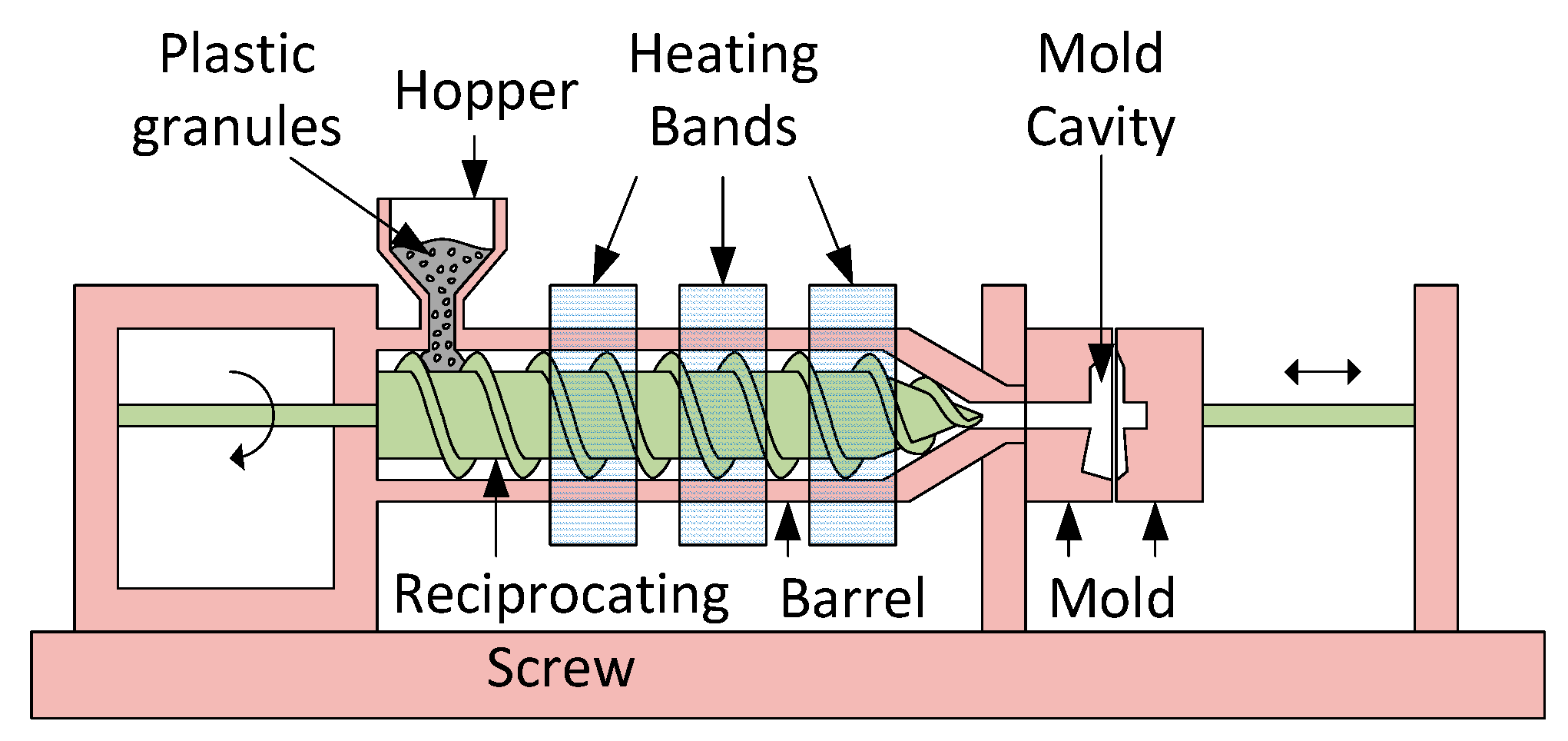
:1. Introduction
2. ANN Controller Design
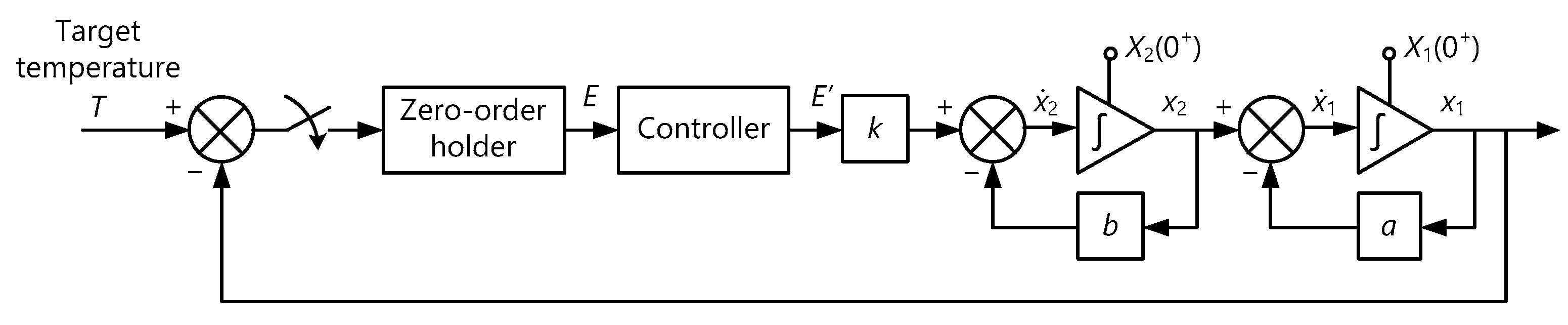
2.1. Reference Digital Controller Design
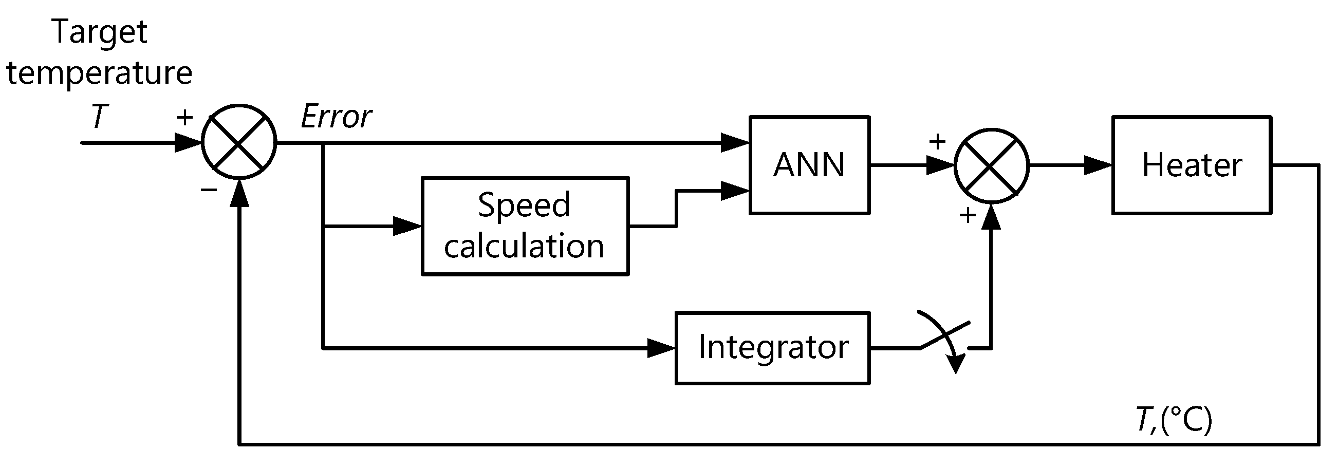
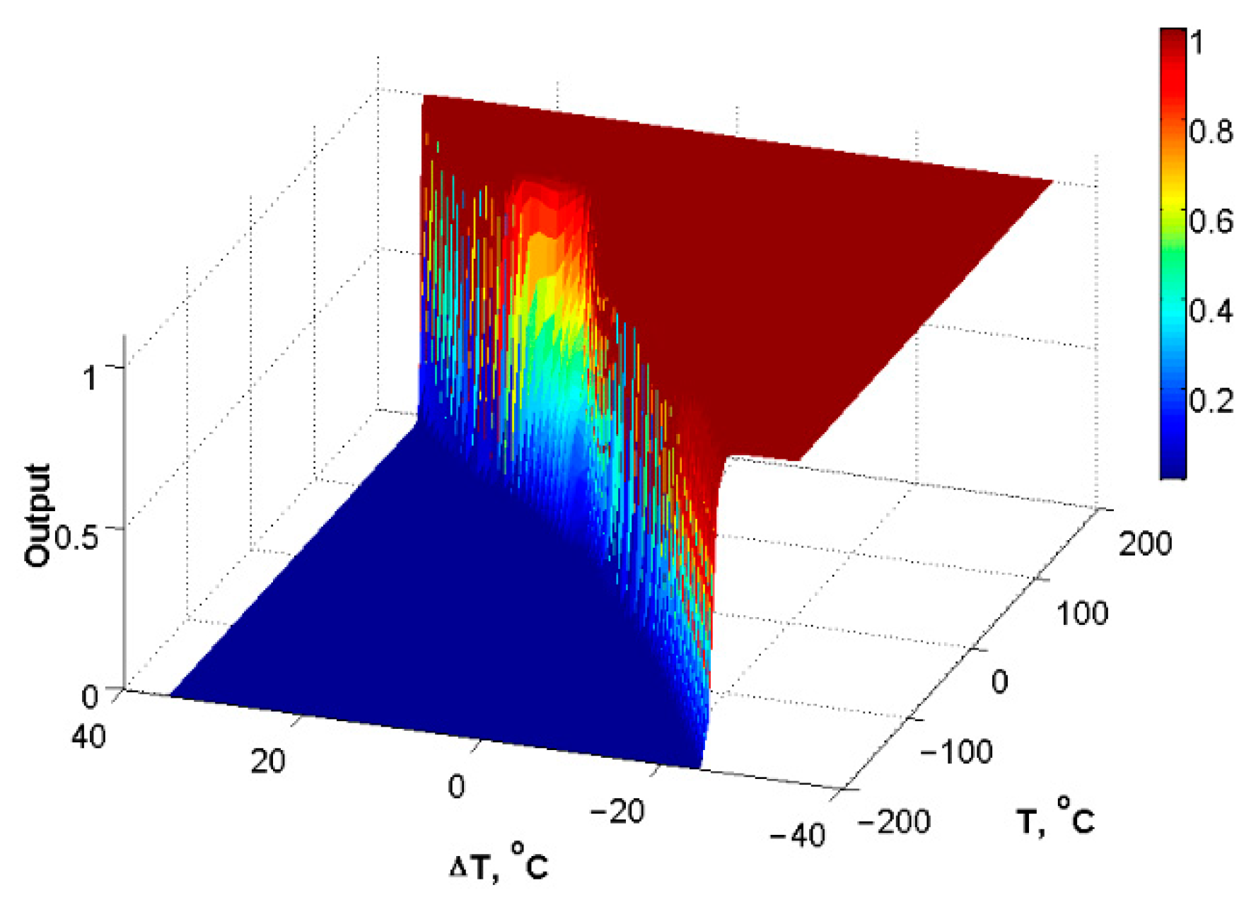
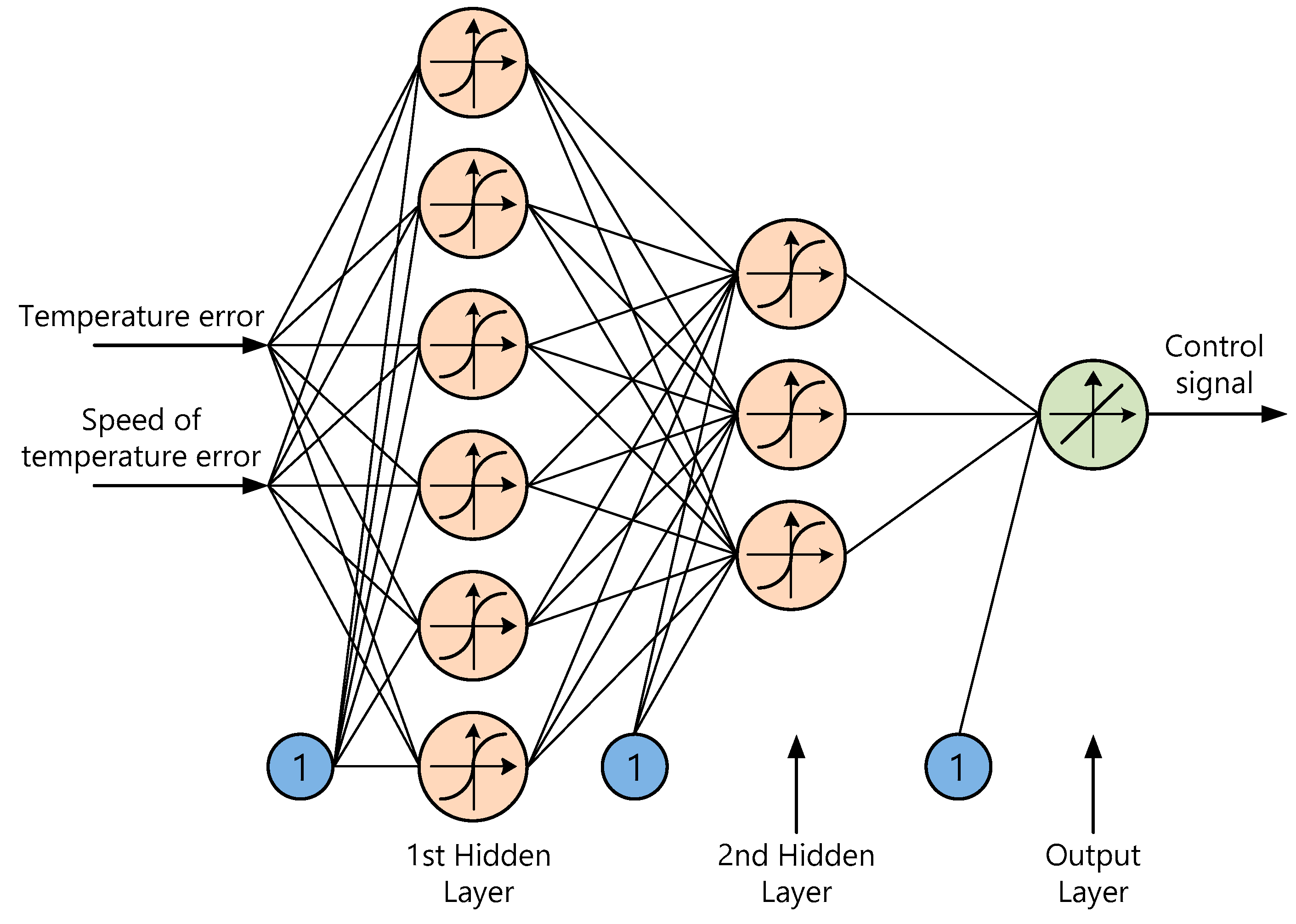
2.2. ANN Structure and Training
- Firstly, the maximum and minimum values of temperature should be selected;
- Then, the duration of both control steps is calculated using Equation (21) for the maximum given temperature;
- The plant response is calculated using transfer Equation (5) for each sampling period of the system. The error is calculated as a difference between the given and current temperatures. The speed of the error varying is calculated as a difference between the current and previous errors (the distance between error values used for speed calculation could be bigger than one sampling period, it depends on the sampling rate and plant dynamic properties);
- The values of errors and speed are stored in two-dimensional input array. The values of control signal, which are “1” for the first control step and “0” for the second, are stored in the output array;
- The target temperature is decremented in the given amount of degrees and process repeats from stage 2 of this algorithm, but on stage 4 the data is placed at the end of the input and output arrays;
- The algorithm stops when the minimum temperature chosen at the first stage is achieved.
3. Matlab Simulation and Experimental Validation
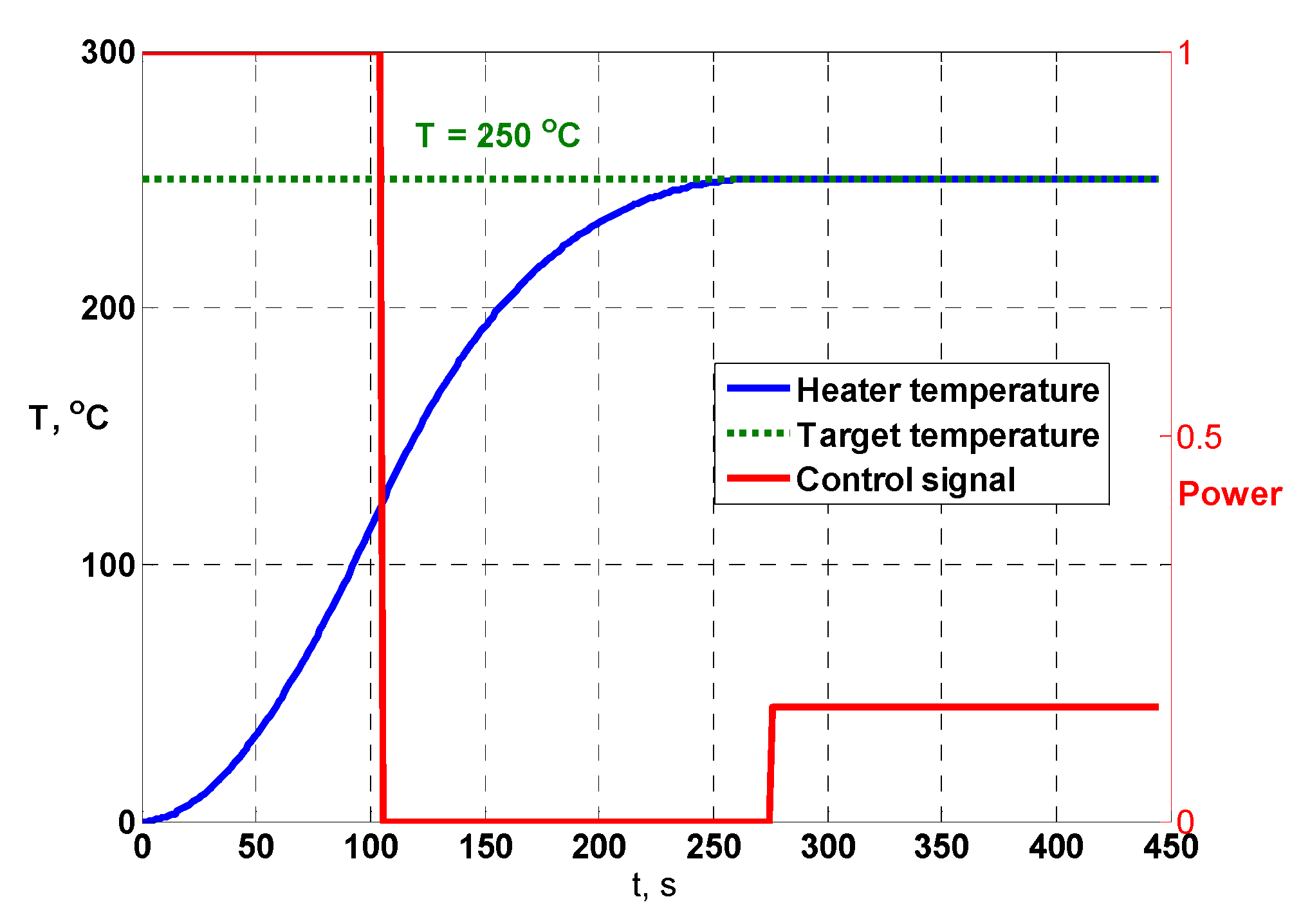
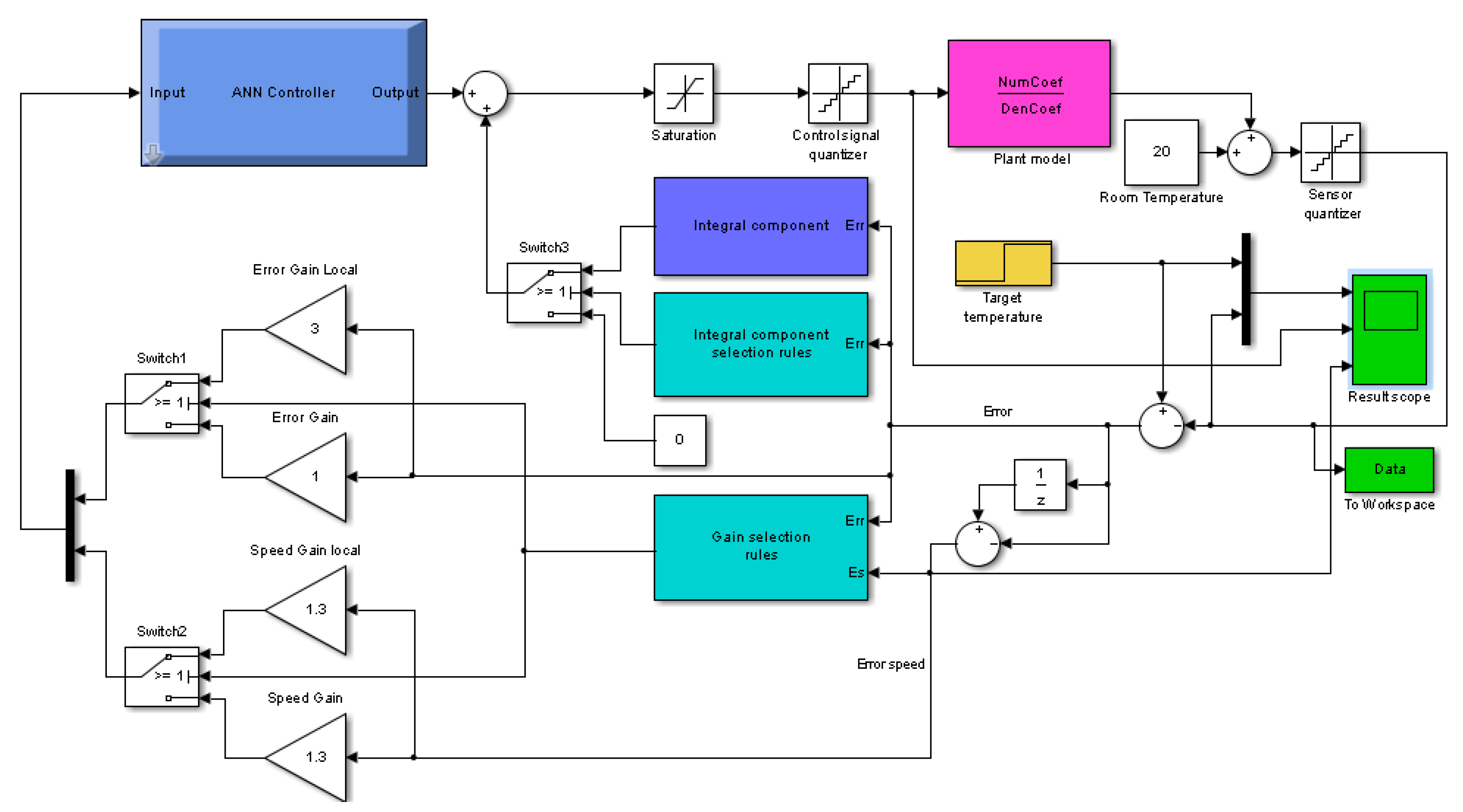
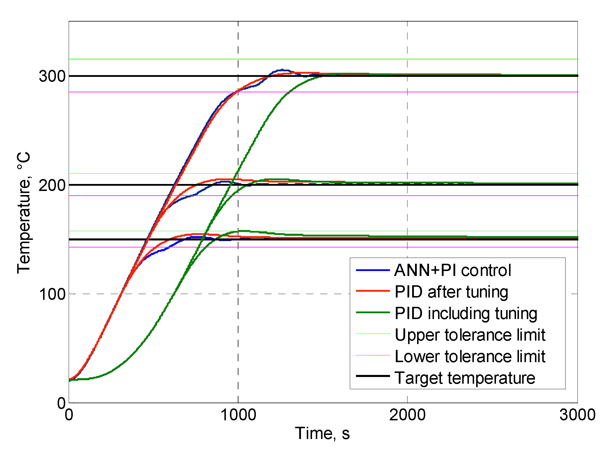
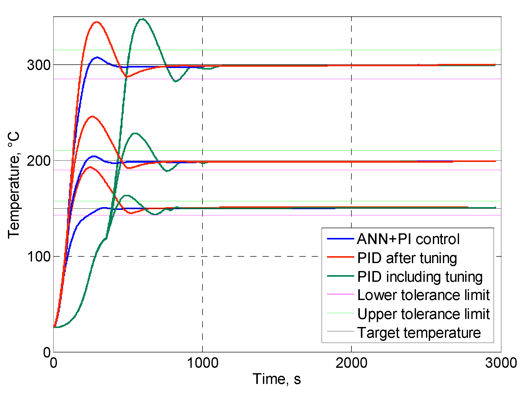
3.1. Matlab Simulation
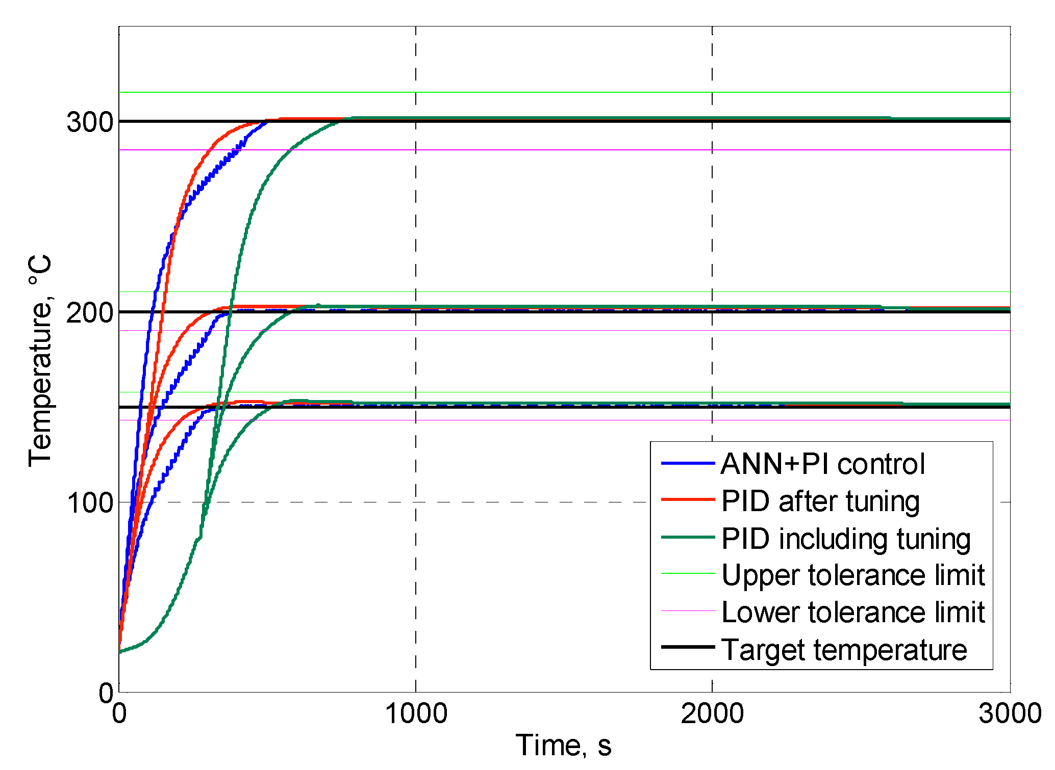
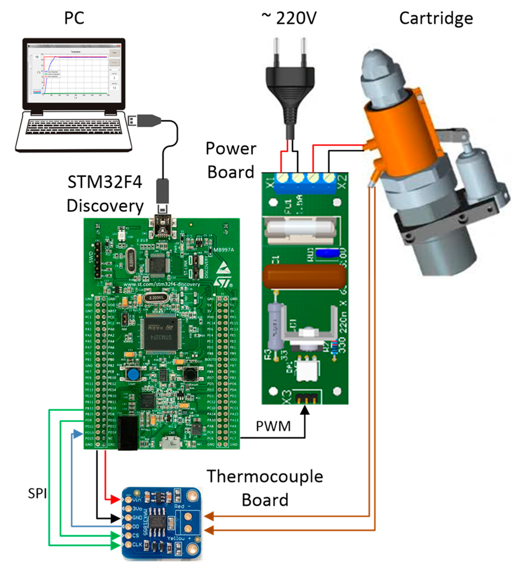
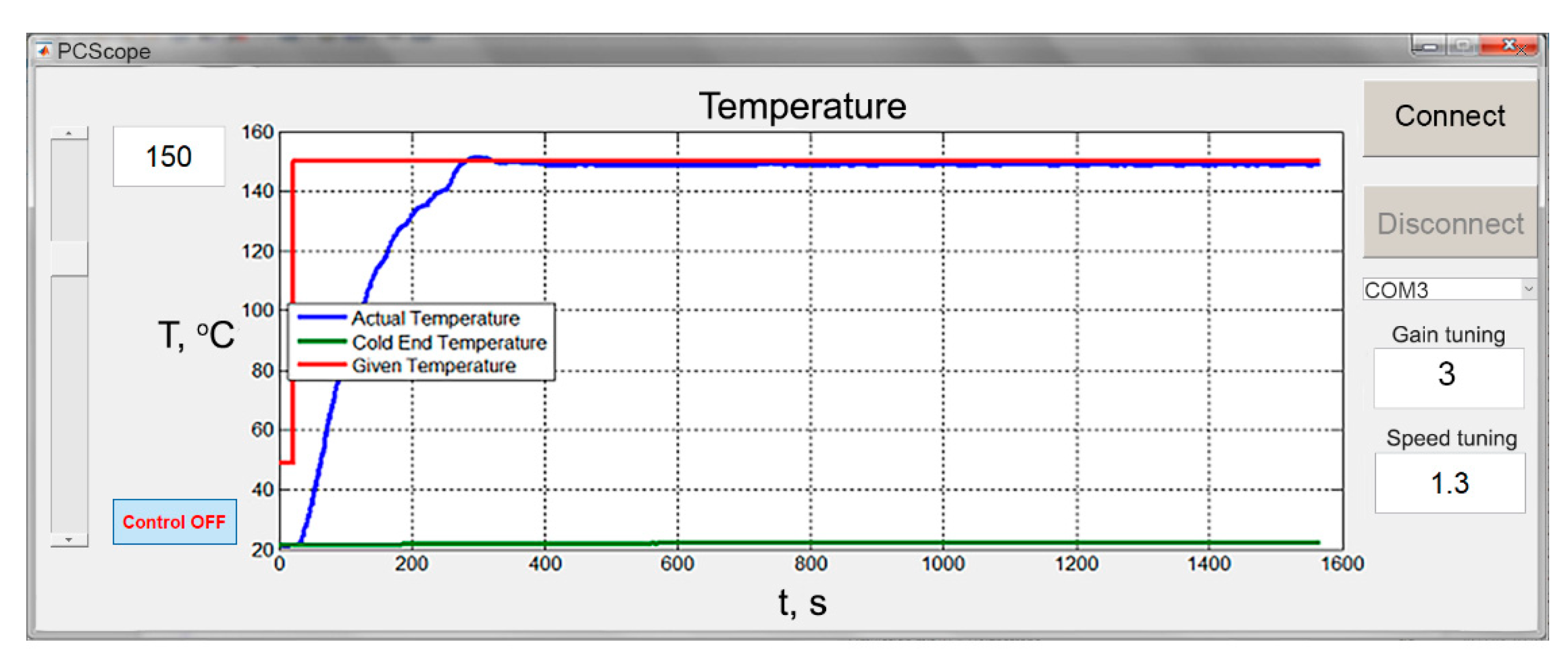
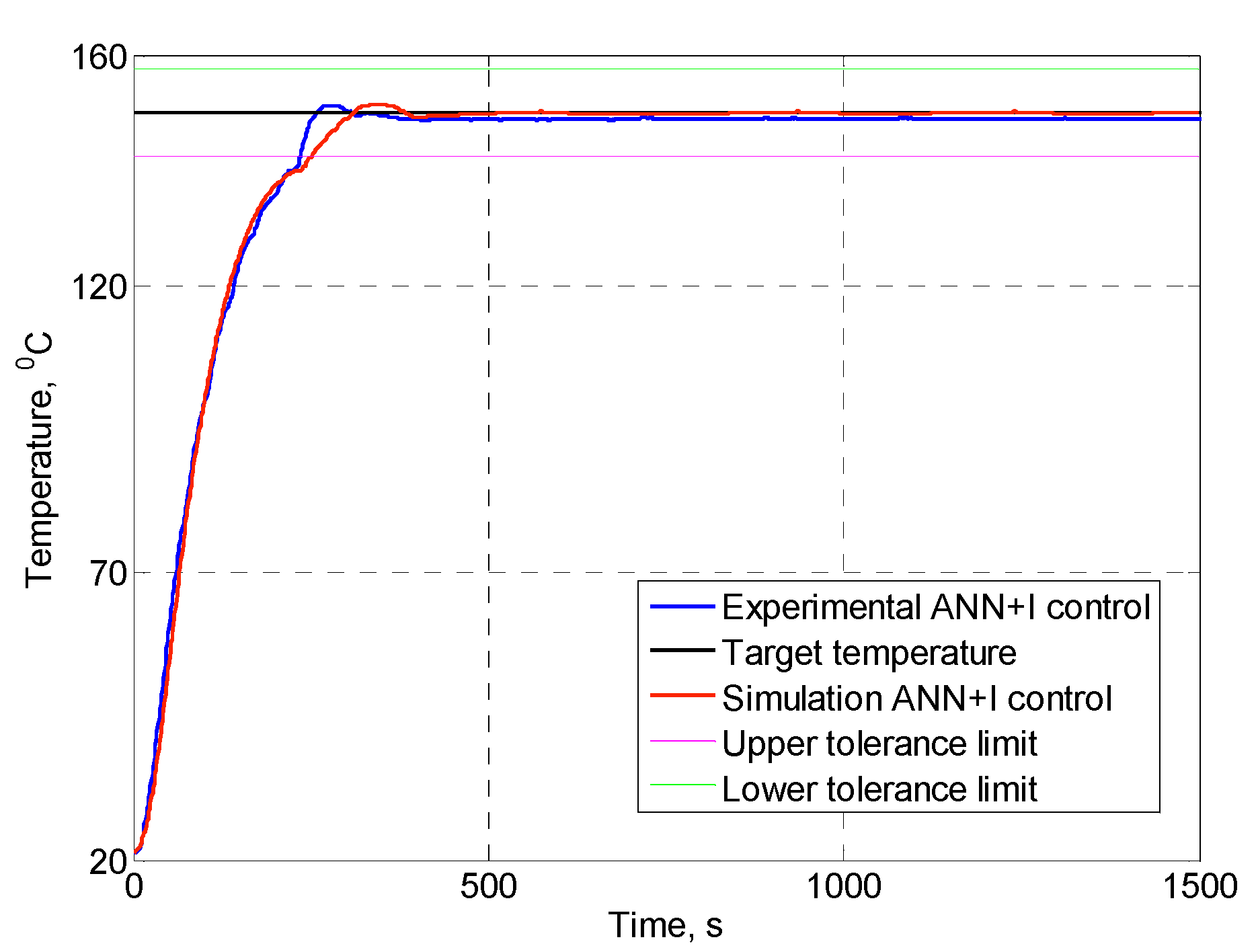
3.2. Experimental Validation
4. Conclusions
Author Contributions
Funding
Conflicts of Interest
References
- Diduch, C.; Dubay, R.; Li, W.G. Temperature control of injection molding. Part I: Modeling and identification. Polym. Eng. Sci. 2004, 44, 2308–2317. [Google Scholar] [CrossRef]
- Spina, R.; Spekowius, M.; Dahlmann, R.; Hopmann, C. Analysis of polymer crystallization and residual stresses in injection molded parts. Int. J. Precis. Eng. Manuf. 2014, 15, 89–96. [Google Scholar] [CrossRef]
- Khomenko, M.; Velihorskyi, O.; Chakirov, R.; Vagapov, Y. Parameters identification of injection plastic moulding heaters. In Proceedings of the 2016 IEEE 36th International Conference on Electronics and Nanotechnology (ELNANO), Kiev, Ukraine, 16 June 2016; pp. 1–6. [Google Scholar]
- Chen, Z.; Turng, L.-S. A review of current developments in process and quality control for injection molding. Adv. Polym. Technol. 2005, 24, 165–182. [Google Scholar] [CrossRef]
- Yao, K.; Gao, F.; Allgower, F. Barrel temperature control during operation transition in injection molding. Control Eng. Pract. 2008, 16, 1259–1264. [Google Scholar] [CrossRef]
- Dubay, R.; Hu, B.; Hernandez, J.M.; Charest, M. Controlling process parameters during plastication in plastic injection molding using model predictive control. Adv. Polym. Technol. 2014, 33. [Google Scholar] [CrossRef]
- Park, H.S.; Phuong, D.X.; Kumar, S. AI based injection molding process for consistent product quality. Procedia Manuf. 2019, 28, 102–106. [Google Scholar] [CrossRef]
- Munoz-Barron, B.; Morales-Velazquez, L.; Romero-Troncoso, R.J.; Rodriguez-Donate, C.; Trejo-Hernandez, M.; Benitez-Rangel, J.P.; Osornio-Ri, R.A. FPGA-based multiprocessor system for injection molding control. Sensors 2012, 12, 14068–14083. [Google Scholar] [CrossRef] [PubMed]
- Chen, S.; Lai, W. Control system software design of injection molding machine based on neural network. In Proceedings of the 2011 Second International Conference on Mechanic Automation and Control Engineering, Hohhot, China, 18 August 2011; pp. 1119–1122. [Google Scholar]
- Lu, C.H.; Tsai, C.C.; Liu, C.M.; Charng, Y.H. Predictive control based on recurrent neural network and application to plastic injection molding processes. In Proceedings of the IECON 2007—33rd Annual Conference of the IEEE Industrial Electronics Society, Taipei, Taiwan, 5–8 November 2007; pp. 792–797. [Google Scholar]
- Selvakarthi, D.; Prasad, S.J.S.; Meenakumari, R.; Balakrishnan, P.A. Optimized temperature controller for plastic injection molding system. In Proceedings of the 2014 International Conference on Green Computing Communication and Electrical Engineering (ICGCCEE), Coimbatore, India, 6–8 March 2014; pp. 1–5. [Google Scholar]
- Tian, D.Z. Main steam temperature control based on GA-BP optimised fuzzy neural network. Int. J. Eng. Syst. Model. Simul. 2017, 9, 150–160. [Google Scholar]
- Ravi, S.; Balakrishnan, P.A. Modelling and control of an anfis temperature controller for plastic extrusion process. In Proceedings of the 2010 International Conference on Communication Control and Computing Technologies, Ramanathapuram, India, 7–9 October 2010; pp. 314–320. [Google Scholar]
- Tou, J.T. Modern Control Theory; McGraw-Hill: New York, NY, USA, 1964. [Google Scholar]
- Khomenko, M.; Voytenko, V.; Vagapov, Y. Neural network-based optimal control of a dc motor positioning system. Int. J. Autom. Control 2013, 7, 83–104. [Google Scholar] [CrossRef]
- Cirstea, M.N.; Dinu, A.; Khor, J.G.; McCormick, M. Neural and Fuzzy Logic Control of Drives and Power Systems; Elsevier Ltd.: Newnes, Australia, 2002. [Google Scholar]
- Haykin, S. Neural Networks: A Comprehensive Foundation, 2nd ed.; Prentice-Hall: Upper Saddle River, NJ, USA, 1999. [Google Scholar]
- Syafaruddin, S.; Hiyama, T.; Karatepe, E. Investigation of ANN performance for tracking the optimum points of PV module under partially shaded conditions. In Proceedings of the 9th International Power and Energy Conference, Singapore, 27–29 October 2010; pp. 1186–1191. [Google Scholar]
- Prokhorov, D.V. Training recurrent neurocontrollers for real-time applications. Ieee Trans. Neural Netw. 2007, 18, 1003–1015. [Google Scholar] [CrossRef] [PubMed]
- Veligorskyi, O.; Chakirov, R.; Khomenko, M.; Vagapov, Y. Artificial neural network motor control for full-electric injection moulding machine. In Proceedings of the IEEE International Conference on Industrial Technology (ICIT), Melbourne, Australia, 13–15 February 2019; pp. 1–5. [Google Scholar]
- Rios-Gutierrez, F.; Makableh, Y.F. Efficient position control of dc servomotor using backpropagation neural network. In Proceedings of the 7th International Conference on Natural Computation, Shanghai, China, 26–28 July 2011; pp. 653–657. [Google Scholar]


| Ttarget,°C | 150 | 200 | 300 | ||||||
|---|---|---|---|---|---|---|---|---|---|
| Control | (I) | (II) | (III) | (I) | (II) | (III) | (I) | (II) | (III) |
| Bar | 872 | 604 | 693 | 1062 | 762 | 853 | 1513 | 1213 | 1186 |
| Nozzle | 523 | 299 | 364 | 590 | 321 | 393 | 753 | 500 | 506 |
| Cartridge | 423 | 126 | 327 | 458 | 148 | 227 | 500 | 192 | 244 |
| Ttarget,°C | 150 | 200 | 300 | ||||||
|---|---|---|---|---|---|---|---|---|---|
| Control | (I) | (II) | (III) | (I) | (II) | (III) | (I) | (II) | (III) |
| Bar | 4.80 | 3.00 | 1.20 | 2.40 | 2.40 | 1.25 | 0.63 | 0.83 | 1.67 |
| Nozzle | 2.07 | 1.53 | 0.20 | 1.40 | 1.40 | 0.15 | 0.67 | 0.33 | 0.10 |
| Cartridge | 8.80 | 28.2 | 0.27 | 13.9 | 22.7 | 1.9 | 15.7 | 14.7 | 2.37 |
© 2019 by the authors. Licensee MDPI, Basel, Switzerland. This article is an open access article distributed under the terms and conditions of the Creative Commons Attribution (CC BY) license (http://creativecommons.org/licenses/by/4.0/).
Share and Cite
Khomenko, M.; Veligorskyi, O.; Chakirov, R.; Vagapov, Y. An ANN-Based Temperature Controller for a Plastic Injection Moulding System. Electronics 2019, 8, 1272. https://doi.org/10.3390/electronics8111272
Khomenko M, Veligorskyi O, Chakirov R, Vagapov Y. An ANN-Based Temperature Controller for a Plastic Injection Moulding System. Electronics. 2019; 8(11):1272. https://doi.org/10.3390/electronics8111272
Chicago/Turabian StyleKhomenko, Maksym, Oleksandr Veligorskyi, Roustiam Chakirov, and Yuriy Vagapov. 2019. "An ANN-Based Temperature Controller for a Plastic Injection Moulding System" Electronics 8, no. 11: 1272. https://doi.org/10.3390/electronics8111272
APA StyleKhomenko, M., Veligorskyi, O., Chakirov, R., & Vagapov, Y. (2019). An ANN-Based Temperature Controller for a Plastic Injection Moulding System. Electronics, 8(11), 1272. https://doi.org/10.3390/electronics8111272