Author Contributions
Conceptualization, M.K., C.A.D., A.S.C. and M.A.A.L.; methodology, E.S., M.K., A.S.C., C.A.D. and M.A.A.L.; software, E.S., M.K. and M.A.A.L.; validation, C.A.D., A.S.C. and A.Y.; formal analysis, C.A.D., A.S.C. and A.Y.; investigation, E.S. M.K. and M.A.A.L.; resources, C.A.D. and A.S.C.; data curation, E.S.; writing–original draft preparation, C.A.D. and A.S.C.; writing–review and editing, E.S. and M.K.; supervision, C.A.D. and A.S.C.; project administration, C.A.D. and A.S.C.; funding acquisition, E.S., M.K., A.S.C., C.A.D., M.A.A.L., and A.Y.
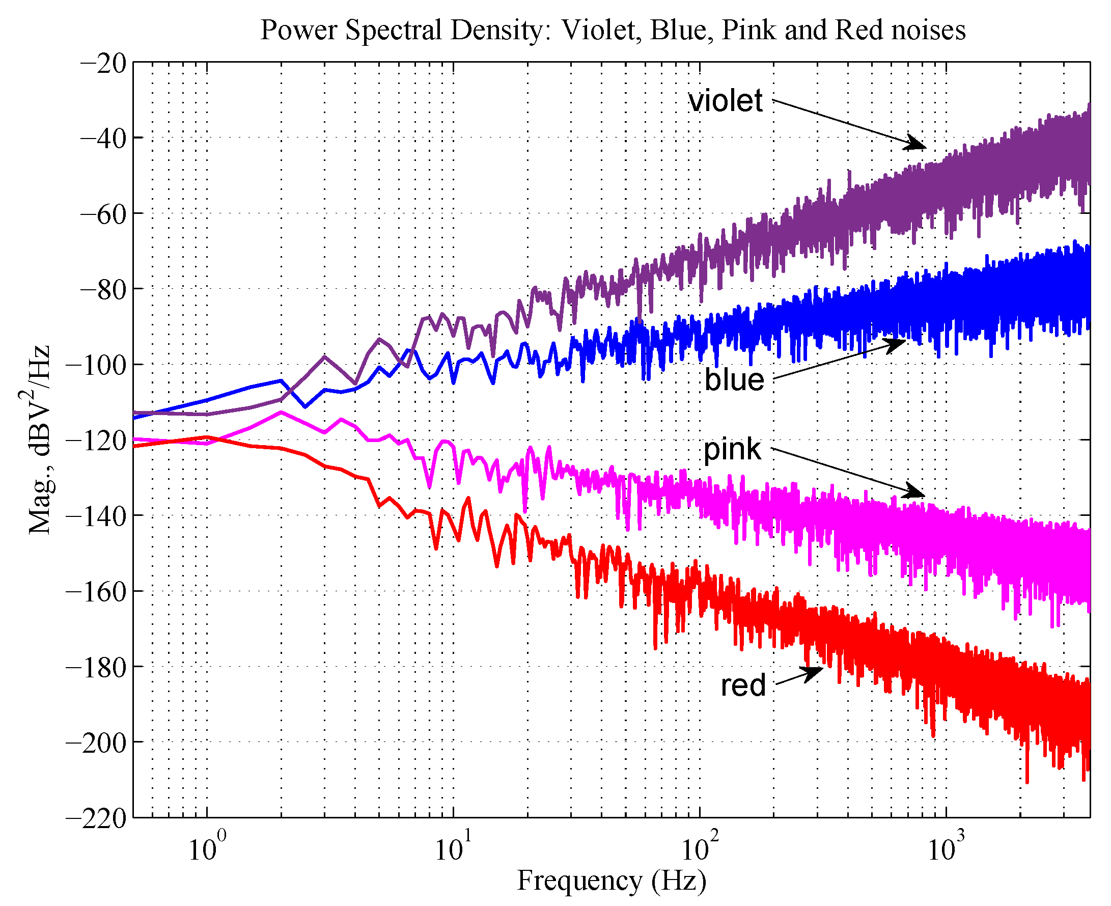
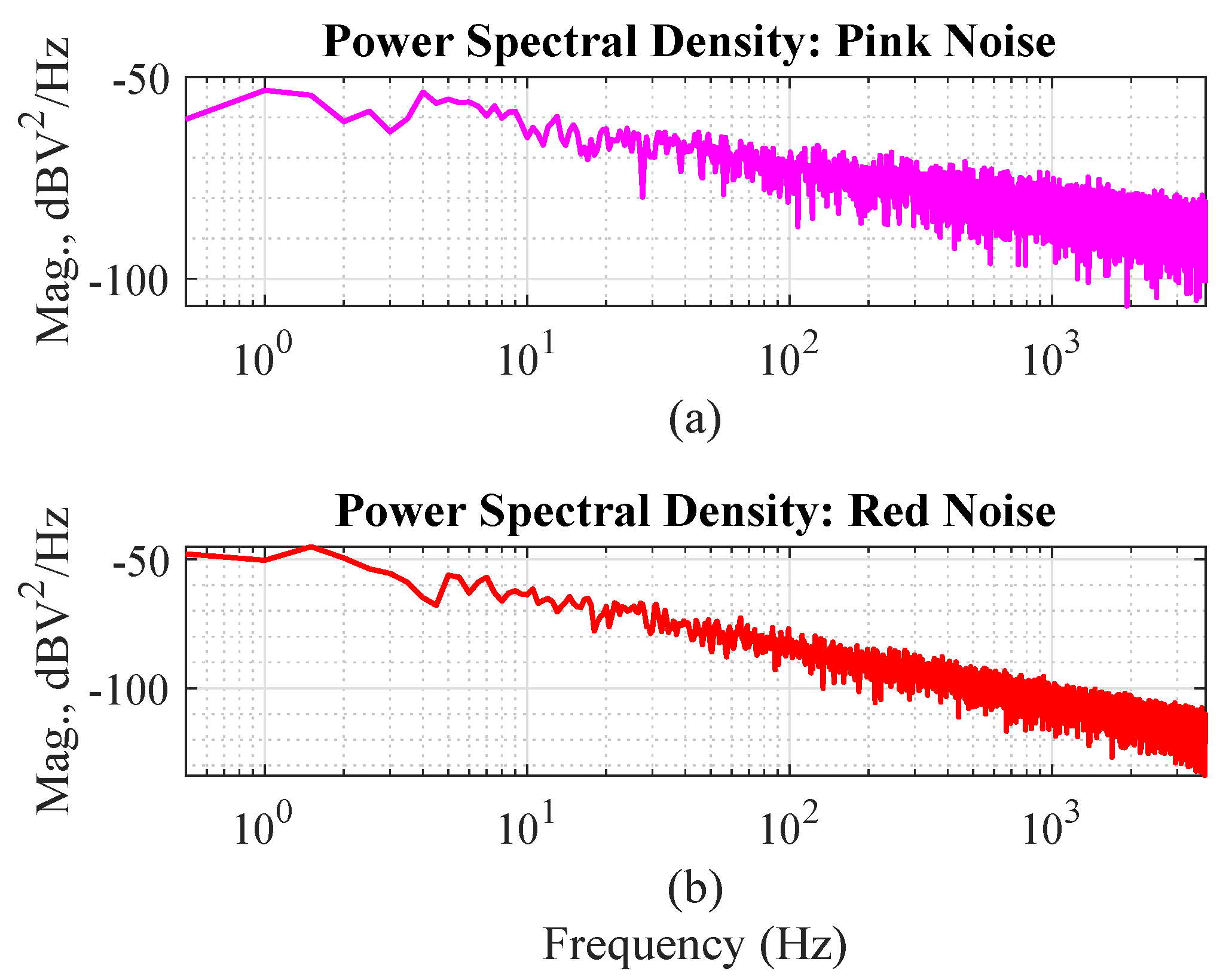
Figure 1.
Power spectral density of violet, blue, pink, and red noises.
Figure 1.
Power spectral density of violet, blue, pink, and red noises.
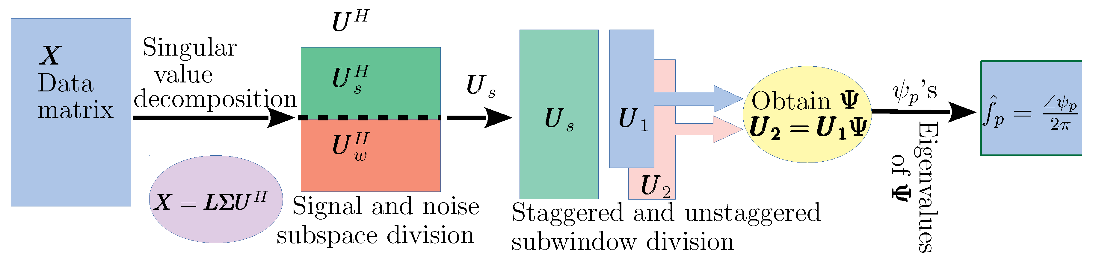
Figure 2.
Demonstrating the block diagram of the ESPRIT algorithm.
Figure 2.
Demonstrating the block diagram of the ESPRIT algorithm.
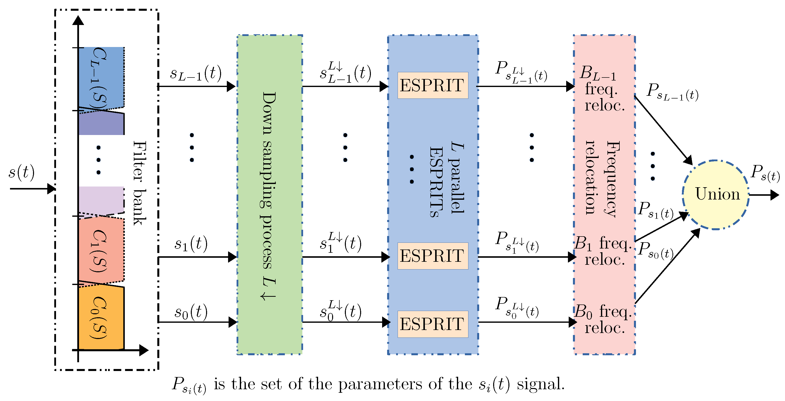
Figure 3.
The filter bank associated ESPRIT block diagram.
Figure 3.
The filter bank associated ESPRIT block diagram.
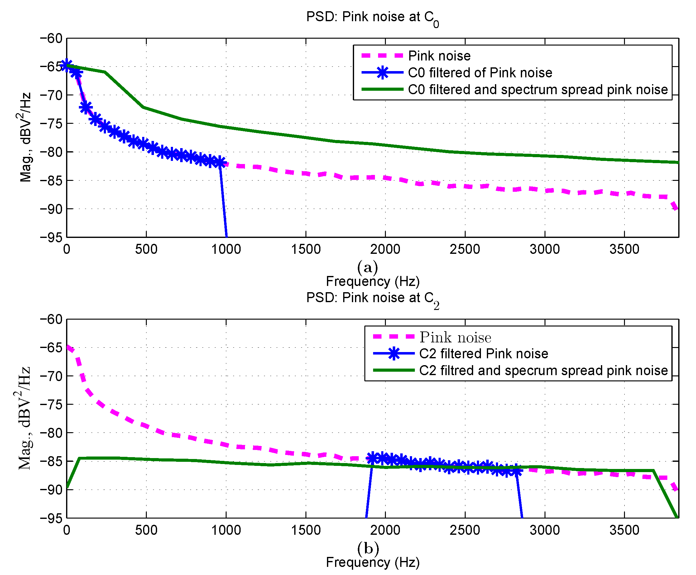
Figure 4.
The stretching effect of the filter bank (FB) followed by spectrum spread inherent to FB-ESPRIT on the pink noise sub-band spectrum; (a) the subband , and (b) the subband after spread spectrum effect.
Figure 4.
The stretching effect of the filter bank (FB) followed by spectrum spread inherent to FB-ESPRIT on the pink noise sub-band spectrum; (a) the subband , and (b) the subband after spread spectrum effect.
Figure 5.
Power spectral density with of the additive (a) pink noise and (b) red noise of dB.
Figure 5.
Power spectral density with of the additive (a) pink noise and (b) red noise of dB.
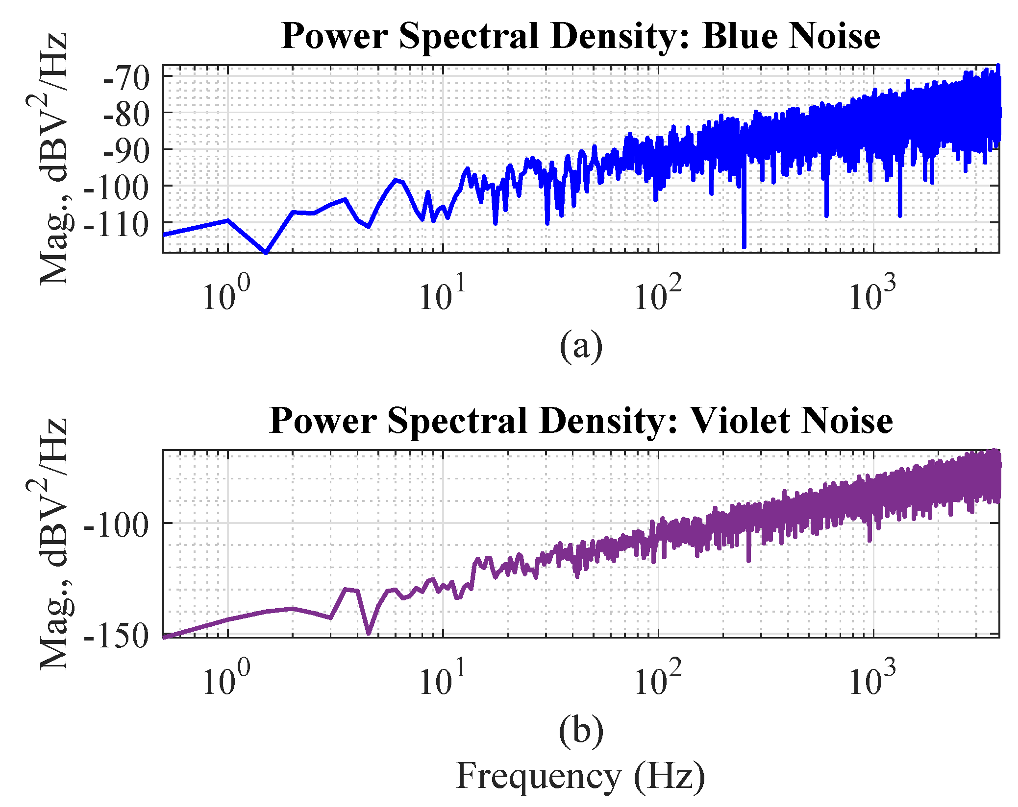
Figure 6.
Power spectral density with of the additive (a) blue noise and (b) violet noise of dB.
Figure 6.
Power spectral density with of the additive (a) blue noise and (b) violet noise of dB.
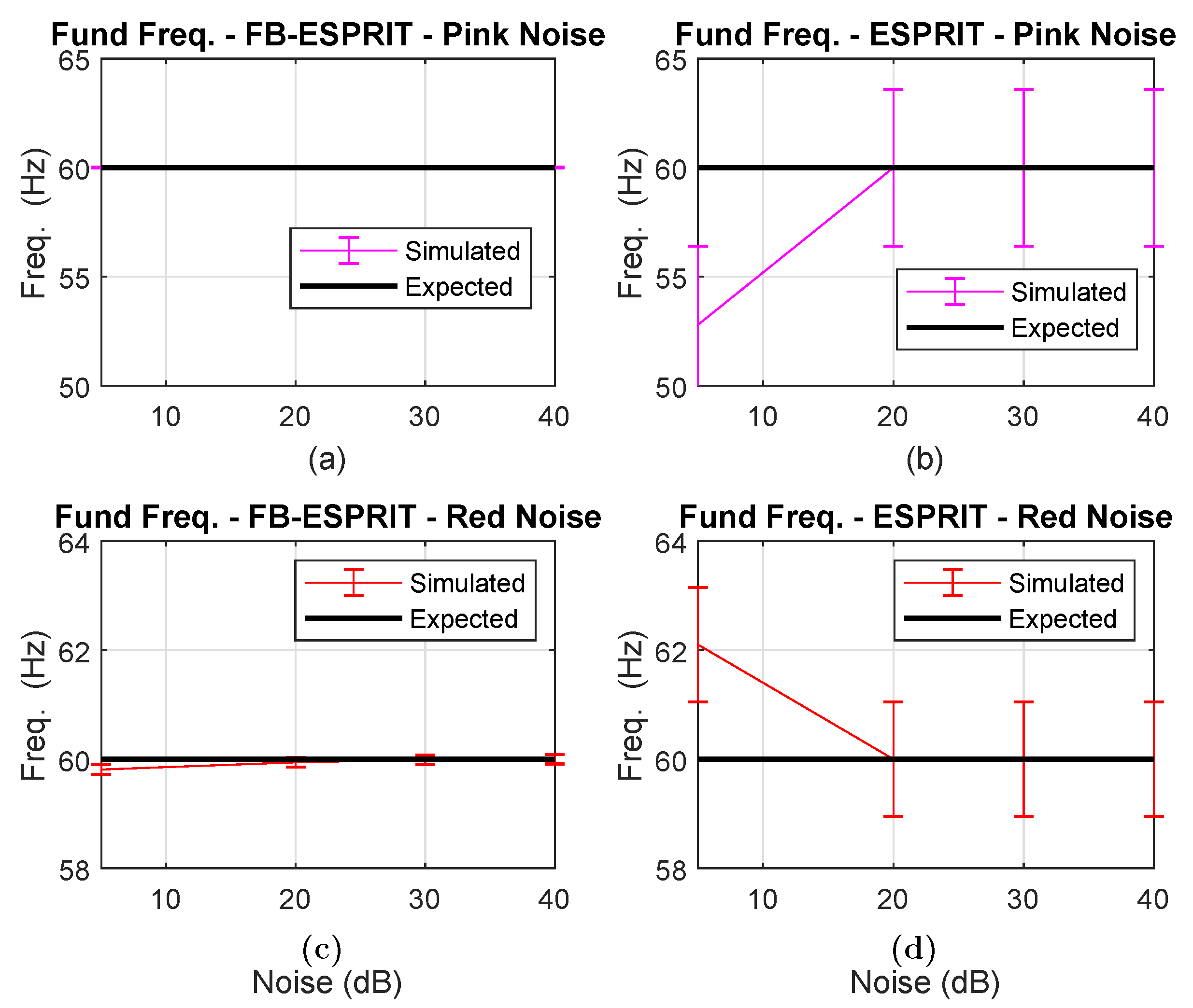
Figure 7.
Estimation of fundamental frequency (Fund Freq.) when is contaminated with pink and red noises; (a) by FB-ESPRIT under pink noise, (b) by ESPRIT under pink noise, (c) by FB-ESPRIT under red noise, and (d) by ESPRIT under red noise.
Figure 7.
Estimation of fundamental frequency (Fund Freq.) when is contaminated with pink and red noises; (a) by FB-ESPRIT under pink noise, (b) by ESPRIT under pink noise, (c) by FB-ESPRIT under red noise, and (d) by ESPRIT under red noise.
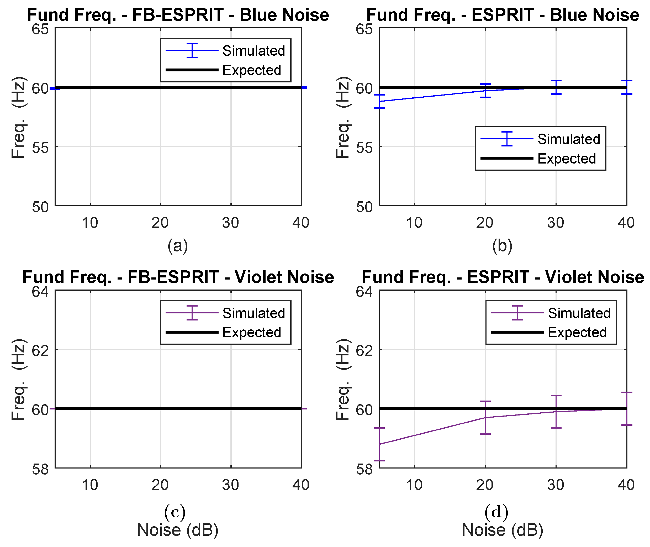
Figure 8.
Estimation of fundamental frequency (Fund Freq.) when is contaminated with blue and violet noises; (a) by FB-ESPRIT under blue noise, (b) by ESPRIT under blue noise, (c) by FB-ESPRIT under violet noise, and (d) by ESPRIT under violet noise.
Figure 8.
Estimation of fundamental frequency (Fund Freq.) when is contaminated with blue and violet noises; (a) by FB-ESPRIT under blue noise, (b) by ESPRIT under blue noise, (c) by FB-ESPRIT under violet noise, and (d) by ESPRIT under violet noise.
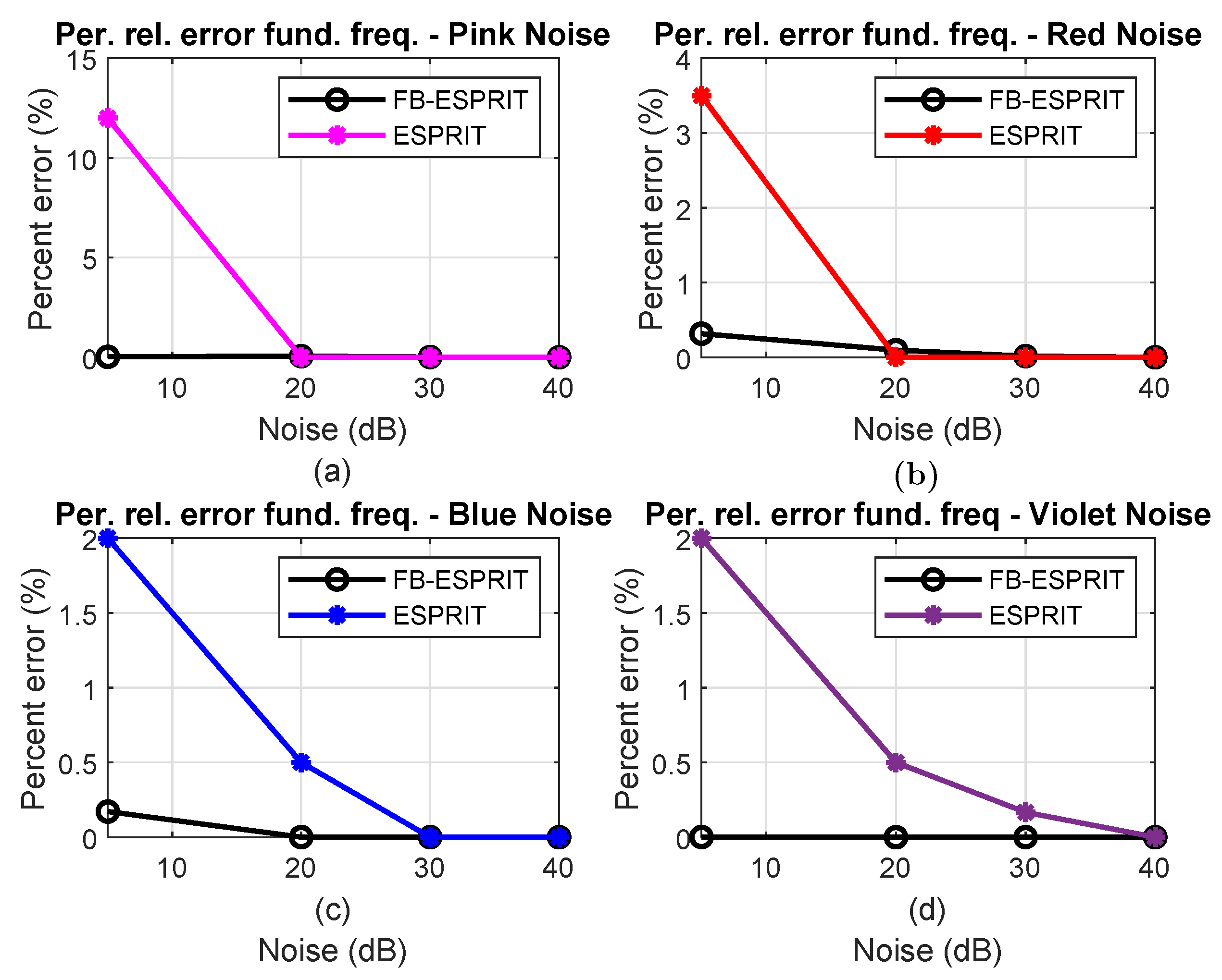
Figure 9.
Percentage of relative (Per. rel.) error (%) of 60 Hz fundamental frequency (fund. freq.) estimation: (a) signal contaminated with pink noise, (b) signal contaminated with red noise, (c) signal contaminated with blue noise, and (d) signal contaminated with violet noise.
Figure 9.
Percentage of relative (Per. rel.) error (%) of 60 Hz fundamental frequency (fund. freq.) estimation: (a) signal contaminated with pink noise, (b) signal contaminated with red noise, (c) signal contaminated with blue noise, and (d) signal contaminated with violet noise.
Figure 10.
Percentage of relative (Per. rel.) error (%) of 60 Hz fundamental component amplitude (fund. amp.): (a) signal contaminated with pink noise; (b) signal contaminated with red noise; (c) signal contaminated with blue noise; (d) signal contaminated with violet noise.
Figure 10.
Percentage of relative (Per. rel.) error (%) of 60 Hz fundamental component amplitude (fund. amp.): (a) signal contaminated with pink noise; (b) signal contaminated with red noise; (c) signal contaminated with blue noise; (d) signal contaminated with violet noise.
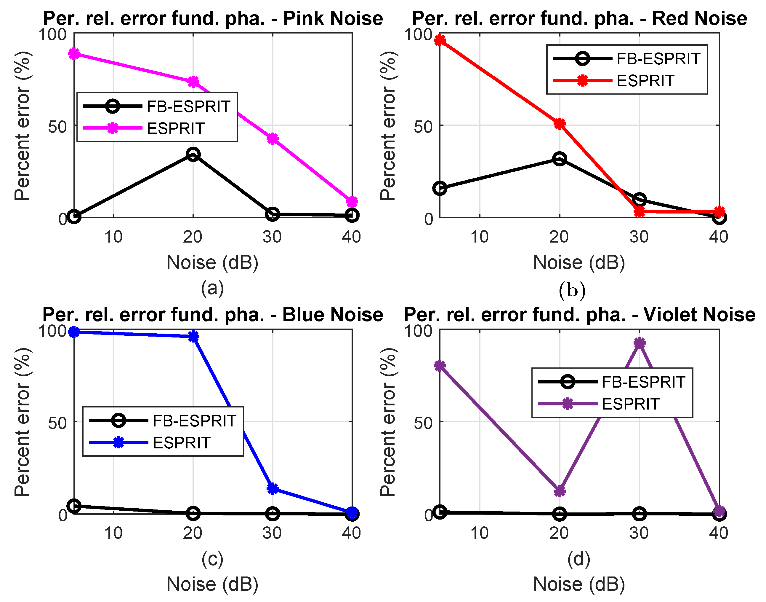
Figure 11.
Percentage relative (Per. rel.) error (%) of 60 Hz fundamental component phase: (a) signal contaminated with pink noise, (b) signal contaminated with red noise, (c) signal contaminated with blue noise, (d) signal contaminated with violet noise.
Figure 11.
Percentage relative (Per. rel.) error (%) of 60 Hz fundamental component phase: (a) signal contaminated with pink noise, (b) signal contaminated with red noise, (c) signal contaminated with blue noise, (d) signal contaminated with violet noise.
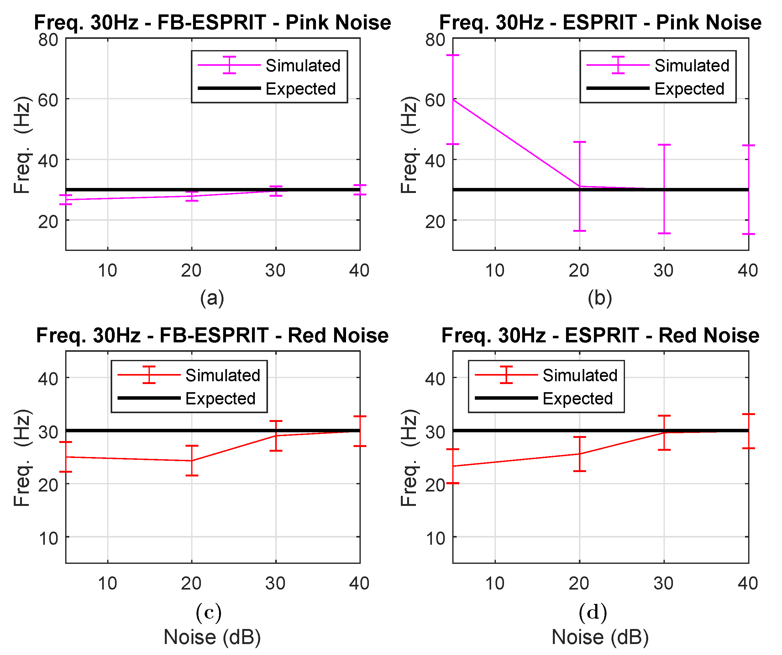
Figure 12.
Estimation of the 30 Hz sub-harmonic frequency of the signal contaminated with pink and red noises, indicating statistical deviations for variation from 5 to 40 dB: (a) by FB-ESPRIT under pink noise, (b) by ESPRIT under pink noise, (c) by FB-ESPRIT under red noise, and (d) by ESPRIT under red noise.
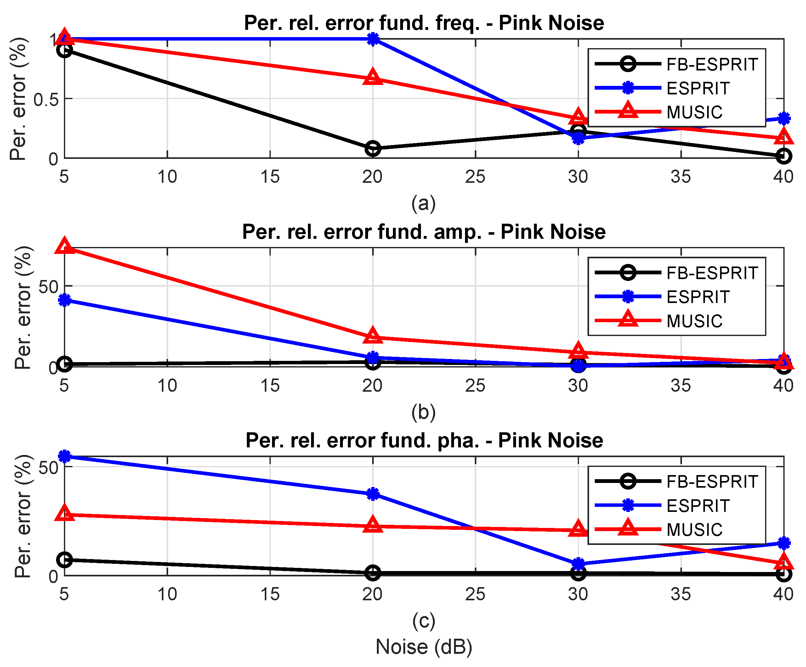
Figure 13.
Percentage error (%) of the 60 Hz fundamental component when the signal is contaminated with pink noise: (a) frequency parameters; (b) amplitude parameters; (c) phase parameters.
Figure 13.
Percentage error (%) of the 60 Hz fundamental component when the signal is contaminated with pink noise: (a) frequency parameters; (b) amplitude parameters; (c) phase parameters.
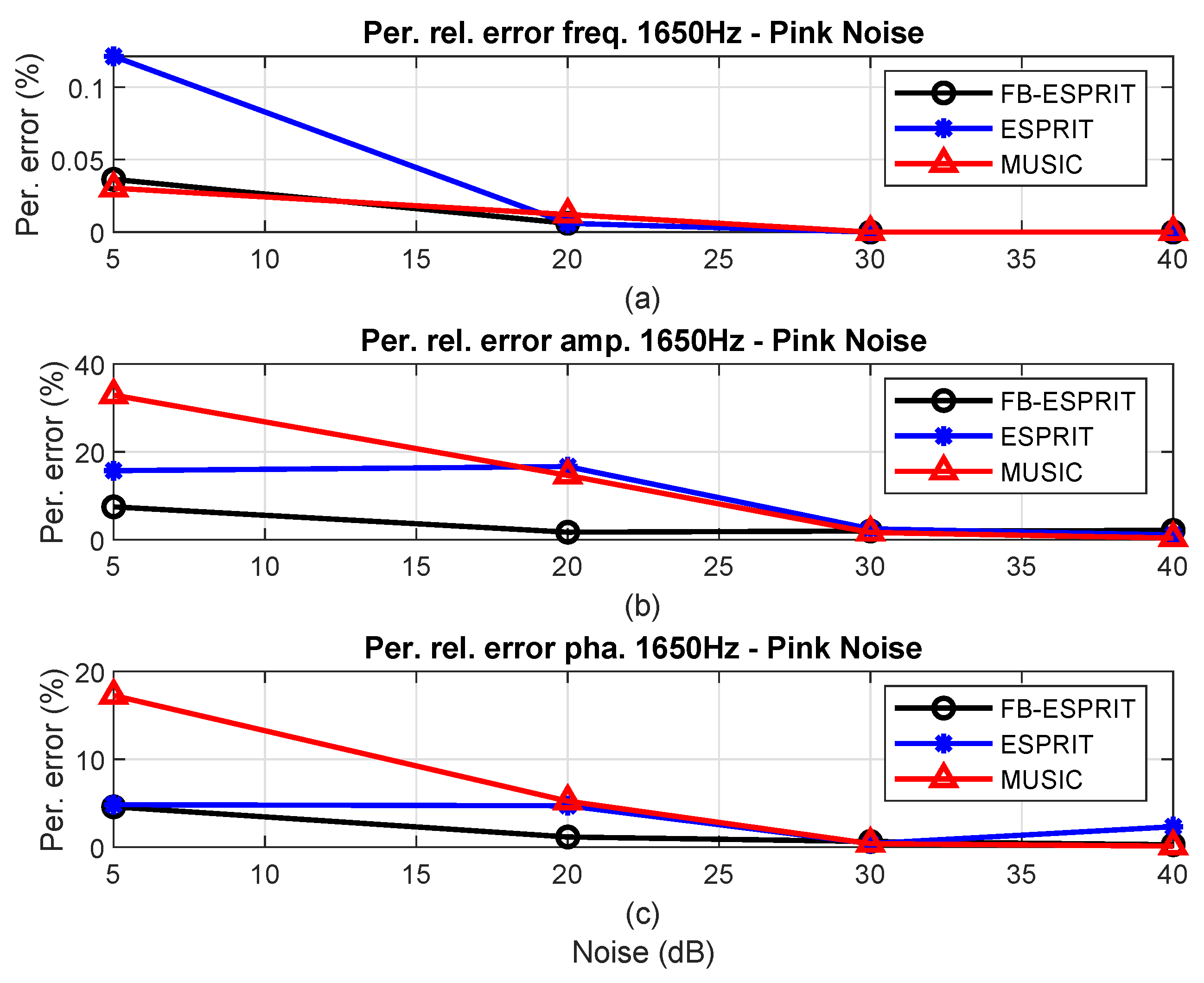
Figure 14.
Percentage error (%) of the 1650 Hz component when signal is contaminated with pink noise: (a) frequency parameters; (b) amplitude parameters; (c) phase parameters.
Figure 14.
Percentage error (%) of the 1650 Hz component when signal is contaminated with pink noise: (a) frequency parameters; (b) amplitude parameters; (c) phase parameters.
Figure 15.
Percentage error (%) of the 2610 Hz component when signal is contaminated with pink noise: (a) frequency parameters; (b) amplitude parameters; (c) phase parameters.
Figure 15.
Percentage error (%) of the 2610 Hz component when signal is contaminated with pink noise: (a) frequency parameters; (b) amplitude parameters; (c) phase parameters.
Figure 16.
Photo-voltaic power plant of the solar laboratory at Federal University of Juiz de Fora (UFJF), Brazil.
Figure 16.
Photo-voltaic power plant of the solar laboratory at Federal University of Juiz de Fora (UFJF), Brazil.
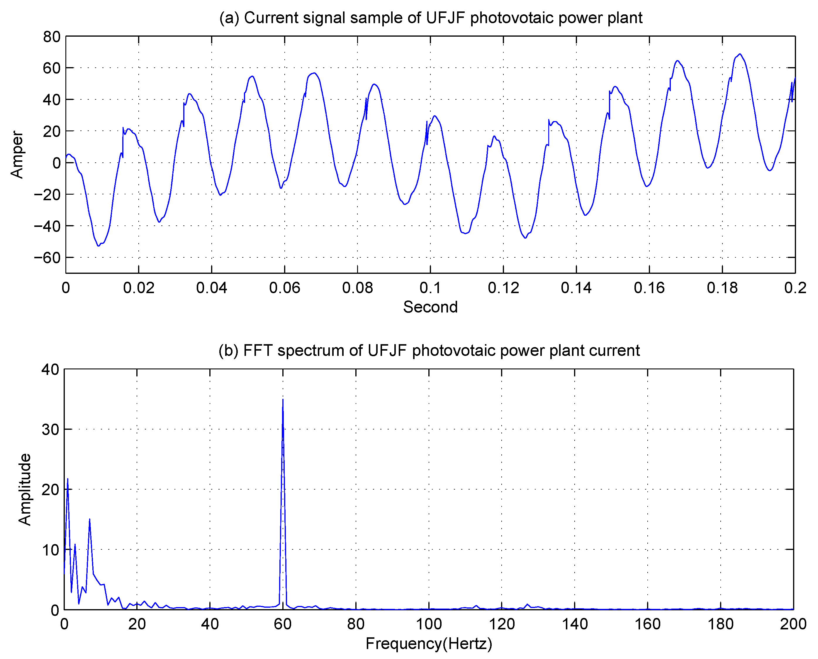
Figure 17.
(a) Two hundred milliseconds of the PV signal measured from the UFJF PV power plant and its (b) FFT spectrum with colored interference in the frequency range of [0–20] Hz.
Figure 17.
(a) Two hundred milliseconds of the PV signal measured from the UFJF PV power plant and its (b) FFT spectrum with colored interference in the frequency range of [0–20] Hz.
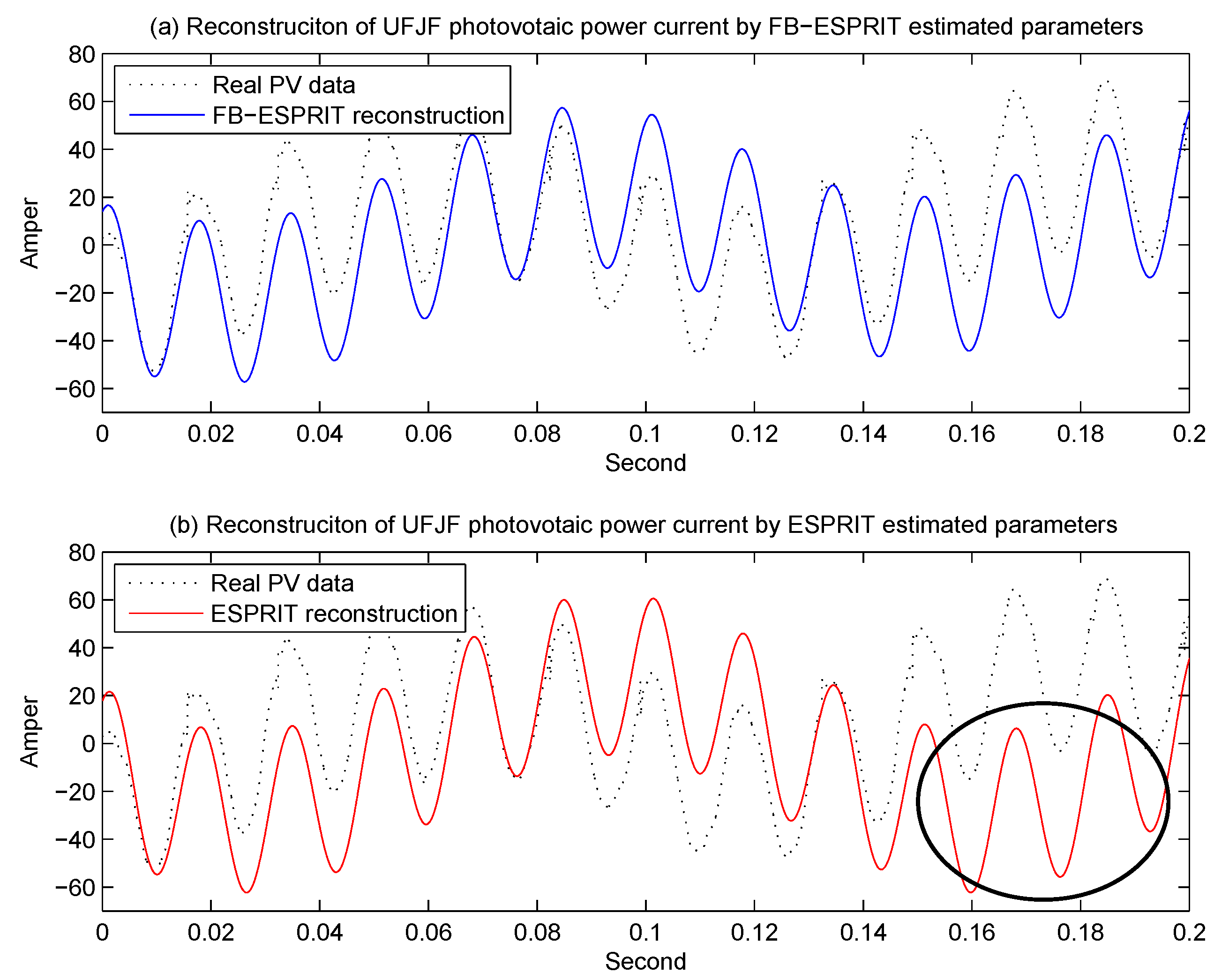
Figure 18.
Original power signal (dashed-black) and the reconstructed signals using the parameters estimated by (a) FB-ESPRIT (solid-blue) and (b) ESPRIT (solid-red).
Figure 18.
Original power signal (dashed-black) and the reconstructed signals using the parameters estimated by (a) FB-ESPRIT (solid-blue) and (b) ESPRIT (solid-red).
Table 1.
Classification of noise according to the power spectral density.
Table 1.
Classification of noise according to the power spectral density.
| Relationship to PSD | Generic Name | Example of Noise |
|---|
| Constant | White Noise | Thermal |
| Proportional to | Pink Noise | Flicker |
| Proportional to | Brown or Red Noise | Popcorn |
| Proportional to f | Blue Noise | x |
| Proportional to | Violet Noise | x |
| Proportional to | No Generic Name | Galactic Noise |
| Irregular form | No Generic Name | Atmospheric Noise |
Table 2.
Mean of signal parameters estimated in 1000 runs for the FB-ESPRIT method and the conventional ESPRIT at different SNR levels (5, 20, 30, 40 dB) of pink noise.
Table 2.
Mean of signal parameters estimated in 1000 runs for the FB-ESPRIT method and the conventional ESPRIT at different SNR levels (5, 20, 30, 40 dB) of pink noise.
| SNR | 5 dB | 20 dB | 30 dB | 40 dB |
|---|
| Estimator | FB-ESP. | ESPRIT | FB-ESP. | ESPRIT | FB-ESP. | ESPRIT | FB-ESP. | ESPRIT |
|---|
| Fund. F. : 60 Hz | 60.02 | 52.80 | 59.96 | 60.00 | 59.99 | 60.00 | 60.00 | 60.00 |
| Int. F. : 30 Hz | 26.71 | 87.70 | 27.87 | 31.10 | 29.56 | 30.20 | 29.97 | 30.00 |
| Har. F.: 1650 | 1649.90 | 1649.00 | 1650.00 | 1650.00 | 1650.00 | 1650.00 | 1650.00 | 1650.00 |
| Har. F.: 2610 | 2610.60 | 2608.90 | 2610.00 | 2610.00 | 2610.00 | 2610.00 | 2610.00 | 2610.00 |
| Har. F.: 3300 | 3299.70 | 227.10 | 3300.00 | 3300.00 | 3300.00 | 3300.00 | 3300.00 | 3300.00 |
| Fund. 60 A.: 1 | 1.06 | 0.70 | 0.96 | 0.91 | 0.99 | 1.10 | 1.01 | 1.07 |
| Int. 30 A.: | 0.18 | 0.08 | 0.20 | 0.34 | 0.20 | 0.40 | 0.20 | 0.21 |
| Har. 1650 A.: | 0.29 | 0.05 | 0.29 | 0.30 | 0.29 | 0.30 | 0.29 | 0.30 |
| Har. 2610 A.: | 0.20 | 0.16 | 0.20 | 0.21 | 0.20 | 0.20 | 0.20 | 0.20 |
| Har. 3300 A.: | 0.09 | 0.08 | 0.10 | 0.11 | 0.10 | 0.10 | 0.10 | 0.10 |
| Fund. 60 : | 15.09 | 1.68 | 20.15 | 3.95 | 15.28 | 8.58 | 15.20 | 13.72 |
| Sub. 30 : | 23.95 | 26.91 | 26.73 | 52.20 | 27.32 | 39.18 | 26.77 | 0,10 |
| Int. 1650 : | 43.05 | 53.06 | 49.90 | 81.98 | 46.96 | 47.00 | 44.88 | 45.21 |
| Har. 2610 : | 57.14 | 55.79 | 64.61 | 61.17 | 56.54 | 61.04 | 61.61 | 60.12 |
| Har. 3300 : | 68.47 | 86.77 | 68.80 | 66.44 | 69.12 | 70.04 | 67.92 | 68.24 |
Table 3.
Percentage error (%) of signal parameters’ estimated with 1000 runs for the FB-ESPRIT method and the conventional ESPRIT method at different SNR levels (5, 20, 30, 40 dB) of pink noise.
Table 3.
Percentage error (%) of signal parameters’ estimated with 1000 runs for the FB-ESPRIT method and the conventional ESPRIT method at different SNR levels (5, 20, 30, 40 dB) of pink noise.
| SNR | 5 dB | 20 dB | 30 dB | 40 dB |
|---|
| Estimator | FB-ESP. | ESPRIT | FB-ESP. | ESPRIT | FB-ESP. | ESPRIT | FB-ESP. | ESPRIT |
|---|
| Fund. F: 60 Hz | 0.03 | 12.00 | 0.06 | 0.00 | 0.01 | 0.00 | 0.00 | 0.00 |
| Int. F.: 30 Hz | 10.97 | 99.00 | 7.09 | 3.67 | 1.45 | 0.67 | 0.09 | 0.00 |
| Har. F.: 1650 | 0.01 | 0.06 | 0.00 | 0.00 | 0.00 | 0.00 | 0.00 | 0.00 |
| Har. F.: 2610 | 0.02 | 0.04 | 0.00 | 0.00 | 0.00 | 0.00 | 0.00 | 0.00 |
| Har. F.: 3300 | 0.01 | 93.12 | 0.00 | 0.00 | 0.00 | 0.00 | 0.00 | 0.00 |
| midrule Fund. 60 A.: 1 | 5.57 | 29.94 | 4.31 | 8.86 | 0.52 | 6.96 | 0.59 | 7.40 |
| Int. 30 A.: | 12.40 | 58.00 | 1.15 | 70.95 | 0.45 | 97.75 | 0.75 | 6.50 |
| Har. 1650 A.: | 3.70 | 83.10 | 2.87 | 1.60 | 2.17 | 0.83 | 2.77 | 0.43 |
| Har. 2610 A.: | 1.80 | 20.95 | 0.45 | 5.00 | 1.15 | 0.15 | 0.20 | 2.60 |
| Har. 3300 A.: | 7.70 | 15.20 | 1.10 | 7.70 | 1.10 | 1.30 | 0.60 | 0.70 |
| Fund. 60 : | 0.58 | 88.81 | 34.31 | 73.65 | 1.89 | 42.77 | 1.31 | 8.56 |
| Sub. 30 : | 4.18 | 7.62 | 6.91 | 96.78 | 9.29 | 56.73 | 7.09 | 99.60 |
| Int. 1650 : | 4.34 | 17.91 | 10.89 | 82.18 | 4.35 | 4.44 | 0.,27 | 0.47 |
| Har. 2610 : | 4.77 | 7.01 | 7.68 | 1.96 | 5.76 | 1.73 | 2.69 | 0.19 |
| Har. 3300 : | 0.69 | 27.60 | 1.17 | 2.30 | 1.65 | 3.01 | 0.12 | 0.35 |
Table 4.
Percent error (%) in signal parameters’ estimation in 1000 runs by FB-ESPRIT and the conventional ESPRIT method at different SNR levels (5, 20, 30, 40 dB) under contamination of red noise.
Table 4.
Percent error (%) in signal parameters’ estimation in 1000 runs by FB-ESPRIT and the conventional ESPRIT method at different SNR levels (5, 20, 30, 40 dB) under contamination of red noise.
| SNR | 5 dB | 20 dB | 30 dB | 40 dB |
|---|
| Estimator | FB-ESP. | ESPRIT | FB-ESP. | ESPRIT | FB-ESP. | ESPRIT | FB-ESP. | ESPRIT |
|---|
| Fund. F: 60 Hz | 0.32 | 3.50 | 0.09 | 0.00 | 0.02 | 0.00 | 0.00 | 0.00 |
| Int. F. : 30 Hz | 16.55 | 22.33 | 18.93 | 14.67 | 3.22 | 1.33 | 0.32 | 0.33 |
| Har. F.: 1650 | 0.00 | 0.01 | 0.00 | 0.00 | 0.00 | 0.00 | 0.00 | 0.00 |
| Har. F.: 2610 | 0.00 | 0.01 | 0.00 | 0.00 | 0.00 | 0.00 | 0.00 | 0.00 |
| Har. F.: 3300 | 0.00 | 81.18 | 0.00 | 0.00 | 0.00 | 0.00 | 0.00 | 0.00 |
| Fund. 60 A.: 1 | 0.62 | 62.29 | 1.21 | 7.40 | 0.63 | 1.23 | 0.09 | 0.17 |
| Int. 30 A.: | 19.20 | 82.80 | 0.25 | 78.95 | 0.70 | 11.15 | 3.40 | 5.00 |
| Har. 1650 A.: | 2.37 | 1.30 | 2.87 | 0.17 | 2.73 | 0.03 | 2.73 | 0.03 |
| Har. 2610 A.: | 0.50 | 0.55 | 0.10 | 0.20 | 0.15 | 0.10 | 0.15 | 0.15 |
| Har. 3300 A.: | 8.70 | 46.00 | 0.80 | 36.90 | 0.80 | 0.10 | 0.70 | 0.00 |
| Fund. 60 : | 15.91 | 96.05 | 31.83 | 50.83 | 9.68 | 3.23 | 0.10 | 3.11 |
| Sub. 30 : | 38.16 | 100.40 | 4.63 | 98.35 | 1.86 | 96.46 | 0.02 | 49.58 |
| Int. 1650 : | 5.56 | 46.01 | 0.67 | 0.94 | 0.80 | 0.19 | 0.84 | 0.03 |
| Har. 2610 : | 5.44 | 4.07 | 2.03 | 0.65 | 0.15 | 0.12 | 0.31 | 0.02 |
| Har. 3300 : | 1.13 | 0.27 | 0.29 | 2.05 | 0.02 | 0.13 | 0.03 | 0.02 |
Table 5.
Percent error (%) in signal parameters’ estimation in 1000 runs by FB-ESPRIT and the conventional ESPRIT method at different SNR levels (5, 20, 30, 40 dB) under contamination of blue noise.
Table 5.
Percent error (%) in signal parameters’ estimation in 1000 runs by FB-ESPRIT and the conventional ESPRIT method at different SNR levels (5, 20, 30, 40 dB) under contamination of blue noise.
| SNR | 5 dB | 20 dB | 30 dB | 40 dB |
|---|
| Estimator | FB-ESP. | ESPRIT | FB-ESP. | ESPRIT | FB-ESP. | ESPRIT | FB-ESP. | ESPRIT |
|---|
| Fund. F.: 60 Hz | 0.17 | 2.00 | 0.00 | 0.50 | 0.00 | 0.00 | 0.00 | 0.00 |
| Int. F. : 30 Hz | 49.53 | NA | 0.01 | NA | 0.00 | 2.00 | 0.00 | 0.00 |
| Har. F.: 1650 | 0.00 | 0.08 | 0.00 | 0.01 | 0.00 | 0.00 | 0.00 | 0.00 |
| Har. F.: 2610 | 0.00 | 0.11 | 0.00 | 0.00 | 0.00 | 0.00 | 0.00 | 0.00 |
| Har. F.: 3300 | 0.00 | 0.43 | 0.00 | 0.01 | 0.00 | 0.00 | 0.00 | 0.00 |
| Fund. 60 A.: 1 | 1.91 | 90.09 | 0.13 | 8.14 | 0.06 | 15.42 | 0.00 | 2.00 |
| Int. 30 A.: | 19.25 | NA | 0.65 | NA | 0.25 | 96.75 | 0.05 | 3.15 |
| Har. 1650 A.: | 3.57 | 88.60 | 1.50 | 1.97 | 2.80 | 1.13 | 2.83 | 0.50 |
| Har. 2610 A.: | 0.20 | 83.40 | 4.30 | 4.35 | 0.55 | 3.90 | 0,70 | 0.75 |
| Har. 3300 A.: | 0.80 | 63.10 | 10.80 | 20.30 | 0.40 | 3.70 | 0.30 | 0.20 |
| Fund. 60 : | 4.32 | 98.57 | 0.30 | 96.13 | 0.10 | 13.72 | 0.02 | 0.77 |
| Sub. 30 : | 22.00 | NA | 1.32 | NA | 0.53 | 28.29 | 0.16 | 28.21 |
| Int. 1650 : | 1.52 | 85.83 | 18.81 | 10.31 | 6.80 | 3.67 | 1.79 | 0.30 |
| Har. 2610 : | 0.35 | 33.10 | 17.43 | 0.54 | 2.13 | 4.36 | 0.12 | 0.39 |
| Har. 3300 : | 0.84 | 32.20 | 2.34 | 40.64 | 1.13 | 0.33 | 0.22 | 1.28 |
Table 6.
Percent error (%) of signal parameters estimated in 1000 runs of the FB-ESPRIT method and the conventional ESPRIT method at different SNR levels (5, 20, 30, 40 dB) while the signal is contaminated with violet noise.
Table 6.
Percent error (%) of signal parameters estimated in 1000 runs of the FB-ESPRIT method and the conventional ESPRIT method at different SNR levels (5, 20, 30, 40 dB) while the signal is contaminated with violet noise.
| SNR | 5 dB | 20 dB | 30 dB | 40 dB |
|---|
| Estimator | FB-ESP. | ESPRIT | FB-ESP. | ESPRIT | FB-ESP. | ESPRIT | FB-ESP. | ESPRIT |
|---|
| Fund. F.: 60 Hz | 0.00 | 2.00 | 0.00 | 0.50 | 0.00 | 0.17 | 0.00 | 0.00 |
| Int. F. : 30 Hz | 0.06 | NA | 0.01 | NA | 0.00 | 11.33 | 0.00 | 0.33 |
| Har. F.: 1650 | 0.01 | 0.14 | 0.00 | 0.01 | 0.00 | 0.00 | 0.00 | 0.00 |
| Har. F.: 2610 | 0.11 | 0.22 | 0.00 | 0.01 | 0.00 | 0.00 | 0.00 | 0.00 |
| Har. F.: 3300 | 0.24 | 1.05 | 0.00 | 0.02 | 0.00 | 0.00 | 0.00 | 0.00 |
| Fund. 60 A.: 1 | 0.44 | 83.96 | 0.01 | 6.96 | 0.02 | 31.43 | 0.03 | 0.64 |
| Int. 30 A.: | 4.25 | NA | 0.01 | NA | 0.10 | 95.00 | 0.10 | 14.55 |
| Har. 1650 A.: | 6.40 | 70.00 | 4.70 | 5.10 | 2.10 | 0.10 | 2.80 | 0.30 |
| Har. 2610 A.: | 17.65 | 81.90 | 9.60 | 12.55 | 0.60 | 2.70 | 0.30 | 0.15 |
| Har. 3300 A.: | 34.90 | 68.50 | 17.10 | 41.20 | 1.00 | 5.30 | 0.80 | 2.20 |
| Fund. 60 : | 1.11 | 80.21 | 0.02 | 12.37 | 0.09 | 92.63 | 0.04 | 1.59 |
| Sub. 30 : | 4.68 | NA | 1.88 | NA | 0.29 | 0.39 | 0.12 | 32.64 |
| Int. 1650 : | 12.89 | 20.71 | 6.39 | 27.65 | 0.23 | 4.63 | 0.01 | 0.17 |
| Har. 2610 : | 3.12 | 8.59 | 0.53 | 1.39 | 0.39 | 3.91 | 0.98 | 0.33 |
| Har. 3300 : | 3.99 | 6.88 | 1.98 | 59.39 | 0.20 | 63.20 | 0.35 | 2.28 |
Table 7.
Mean signal parameters estimated in 1000 runs by FB-ESPRIT, ESPRIT, and MUSIC at different levels of SNR (5, 20, 30, 40 dB) under contamination by pink noise.
Table 7.
Mean signal parameters estimated in 1000 runs by FB-ESPRIT, ESPRIT, and MUSIC at different levels of SNR (5, 20, 30, 40 dB) under contamination by pink noise.
| SNR | 5 dB | 20 dB | 30 dB | 40 dB |
|---|
| Estimator | FB-ESP. | ESPRIT | MUSIC | FB-ESP. | ESPRIT | MUSIC | FB-ESP. | ESPRIT | MUSIC | FB-ESP. | ESPRIT | MUSIC |
|---|
| Fund. F.: 60 Hz | 60.55 | 59.40 | 59.40 | 59.95 | 60.60 | 59.60 | 59.86 | 60.10 | 59.80 | 60.01 | 60.20 | 59.90 |
| Int. F.: 45 Hz | 36.97 | NA | NA | 44.74 | 43.00 | NA | 44.93 | 43.60 | 46.30 | 44.95 | 40.10 | 45.20 |
| Int. F.: 1650 Hz | 1650.60 | 1648.00 | 1649.50 | 1649.90 | 1649.90 | 1649.80 | 1650.00 | 1650.00 | 1650.00 | 1650.00 | 1650.00 | 1650.00 |
| Int. F.: 2610 | 2610.10 | 2610.50 | 2610.70 | 2610.30 | 2610.20 | 2610.00 | 2609.90 | 2610.00 | 2610.00 | 2610.00 | 2609.90 | 2610.00 |
| Har. F.: 3000 | 3003.10 | NA | NA | 2999.90 | 3000.00 | 3000.20 | 3000.10 | 3000.10 | 3000.00 | 3000.00 | 2999.80 | 3000.00 |
| Har. F.: 3780 | 3779.40 | NA | NA | 3780.10 | 3780.10 | 3779.60 | 3780.00 | 3780.10 | 3779.90 | 3780.00 | 3780.00 | 3780.00 |
| Fund. 60 A.: 1 | 1.02 | 1.41 | 1.74 | 1.03 | 0.94 | 1.18 | 0.99 | 1.00 | 1.09 | 1.00 | 1.04 | 1.02 |
| Int. 45 A.: | 0.18 | NA | NA | 0.21 | 0.16 | NA | 0.21 | 0.21 | 0.39 | 0.20 | 0.18 | 0.24 |
| Int. 1650 A.: | 0,28 | 0.35 | 0.40 | 0.29 | 0.35 | 0.34 | 0.29 | 0.29 | 0.30 | 0.29 | 0.30 | 0.30 |
| Int. 2610 A.: | 0.21 | 0.30 | 0.36 | 0.20 | 0.21 | 0.32 | 0.20 | 0.20 | 0.20 | 0.20 | 0.19 | 0.20 |
| Har. 3000 A.: | 0.11 | NA | NA | 0.10 | 0.11 | 0.21 | 0.10 | 0.10 | 0.10 | 0.10 | 0.11 | 0.10 |
| Har. 3780 A.: | 0.11 | NA | NA | 0.10 | 0.09 | 0.12 | 0.10 | 0.10 | 0.10 | 0.10 | 0.10 | 0.11 |
| Fund. 60 : | 23.20 | 11.31 | 31.98 | 25.30 | 15.64 | 30.65 | 24.70 | 23.68 | 30.18 | 24.82 | 21.27 | 26.39 |
| Int. 45 : | 32.10 | NA | NA | 28.00 | 55.70 | NA | 29.42 | 50.56 | 10.21 | 30.48 | 70.56 | 26.92 |
| Int. 1650 : | 47.07 | 47.18 | 52.77 | 45.52 | 47.12 | 42.64 | 45.29 | 44.81 | 44.82 | 44.87 | 43.95 | 45.06 |
| Int. 2610 : | 64.71 | 74.78 | 54.40 | 61.54 | 62.73 | 52.15 | 59.82 | 58.27 | 60.36 | 61.51 | 59.82 | 59.97 |
| Har. 3000 : | 65.48 | NA | NA | 70.13 | 72.25 | 95.80 | 67.86 | 66.74 | 66.20 | 67.99 | 77.56 | 69.06 |
| Har. 3780 : | 47.65 | NA | NA | 49.56 | 58.67 | 46.32 | 49.72 | 48.91 | 51.53 | 50.79 | 48.79 | 48.89 |
Table 8.
Mean percent error (%) of signal parameters estimated in 1000 runs by FB-ESPRIT, ESPRIT, and MUSIC at different levels of SNR (5, 20, 30, 40 dB) under contamination by pink noise.
Table 8.
Mean percent error (%) of signal parameters estimated in 1000 runs by FB-ESPRIT, ESPRIT, and MUSIC at different levels of SNR (5, 20, 30, 40 dB) under contamination by pink noise.
| SNR | 5 dB | 20 dB | 30 dB | 40 dB |
|---|
| Estimator | FB-ESP. | ESPRIT | MUSIC | FB-ESP. | ESPRIT | MUSIC | FB-ESP. | ESPRIT | MUSIC | FB-ESP. | ESPRIT | MUSIC |
|---|
| Fund. F.: 60 Hz | 0.91 | 1.00 | 1.00 | 0.08 | 1.00 | 0.67 | 0.23 | 0.17 | 0.33 | 0.02 | 0.33 | 0.17 |
| Int. F.: 45 Hz | 17.85 | NA | NA | 0.57 | 4.44 | NA | 0.15 | 3.11 | 2.89 | 0.11 | 10.89 | 0.44 |
| Int. F.: 1650 Hz | 0.04 | 0.12 | 0.03 | 0.01 | 0.01 | 0.01 | 0.00 | 0.00 | 0.00 | 0.00 | 0.00 | 0.00 |
| Int. F.: 2610 | 0.00 | 0.02 | 0.03 | 0.01 | 0.01 | 0.00 | 0.00 | 0.00 | 0.00 | 0.00 | 0.00 | 0.00 |
| Har. F.: 3000 | 0.10 | NA | NA | 0.00 | 0.00 | 0.01 | 0.00 | 0.00 | 0.00 | 0.00 | 0.01 | 0.00 |
| Har. F.: 3780 | 0.02 | NA | NA | 0.00 | 0.00 | 0.01 | 0.00 | 0.00 | 0.00 | 0.00 | 0.00 | 0.00 |
| Fund. 60 A.: 1 | 1.70 | 41.22 | 73.56 | 2.95 | 5.65 | 18.15 | 1.29 | 0.42 | 8.92 | 0.37 | 4.09 | 2.35 |
| Int. 45 A.: | 11.50 | NA | NA | 4.25 | 18.45 | NA | 4.40 | 6.40 | 97.05 | 1.95 | 12.10 | 21.60 |
| Int. 1650 A.: | 7.47 | 15.70 | 32.90 | 1.70 | 16.63 | 14.63 | 2.00 | 2.47 | 1.63 | 2.10 | 1.07 | 0.37 |
| Int. 2610 A.: | 7.35 | 51.70 | 78.20 | 1.50 | 3.15 | 59.10 | 0.45 | 0.20 | 2.45 | 0.15 | 5.85 | 0.70 |
| Har. 3000 A.: | 10.20 | NA | NA | 1.90 | 9.70 | 105.60 | 0.40 | 0.50 | 3.50 | 2.40 | 6.00 | 1.00 |
| Har. 3780 A.: | 7.00 | NA | NA | 3.40 | 5.10 | 16.60 | 4.70 | 0.20 | 2.20 | 3.70 | 3.00 | 6.00 |
| Fund. 60 : | 7.21 | 54.74 | 27.91 | 1.20 | 37.45 | 22.59 | 1.18 | 5.28 | 20.73 | 0.73 | 14.90 | 5.58 |
| Int. 45 : | 6.99 | NA | NA | 6.65 | 85.66 | NA | 192 | 68.54 | 65.98 | 1.61 | 135.21 | 10.26 |
| Int. 1650 : | 4.60 | 4.84 | 17.27 | 1.17 | 4.72 | 5.24 | 0.65 | 0.42 | 0.41 | 0.28 | 2.33 | 0.12 |
| Int. 2610 : | 7.85 | 24.63 | 9.34 | 2.56 | 4.56 | 13.09 | 0.30 | 2.89 | 0.60 | 2.51 | 0.29 | 0.05 |
| Har. 3000 : | 3.70 | NA | NA | 3.13 | 6.25 | 40.88 | 0.20 | 1.85 | 2.65 | 0.01 | 14.06 | 1.55 |
| Har. 3780 : | 4.70 | NA | NA | 0.89 | 17.34 | 7.35 | 0.56 | 2.18 | 3.07 | 1.58 | 2.42 | 2.22 |
Table 9.
Percent error (%) in the estimation of the parameters of signal contaminated by pink, red, blue, and violet noises with an SNR of 5 dB in 1000 runs of FB-ESPRIT, ESPRIT, and MUSIC.
Table 9.
Percent error (%) in the estimation of the parameters of signal contaminated by pink, red, blue, and violet noises with an SNR of 5 dB in 1000 runs of FB-ESPRIT, ESPRIT, and MUSIC.
| NOISE | Pink | Red | Blue | Violet |
|---|
| SNR | 5 dB | 5 dB | 5 dB | 5 dB |
|---|
| Estimator | FB-ESP. | ESPRIT | MUSIC | FB-ESP. | ESPRIT | MUSIC | FB-ESP. | ESPRIT | MUSIC | ESP.-BF | ESPRIT | MUSIC |
|---|
| Fund. F.: 60 Hz | 0.91 | 1.00 | 1.00 | 0.92 | 0.17 | 5.00 | 1.01 | 1.00 | 5.00 | 0.01 | 1.00 | 5.00 |
| Int. F.: 45 Hz | 17.85 | NA | NA | 39.20 | NA | 5.67 | 2.37 | NA | 1.17 | 0.82 | NA | 1.17 |
| Int. F.: 1650 Hz | 0.04 | 0.12 | 0.03 | 0.01 | 0.01 | NA | 0.04 | 0.05 | NA | 0.03 | 0.10 | NA |
| Int. F.: 2610 | 0.00 | 0.02 | 0.03 | 0.02 | 0.01 | 0.00 | 0.45 | 0.17 | 0.06 | 0.05 | 0.08 | 0.02 |
| Har. F.: 3000 | 0.10 | NA | NA | 0.02 | NA | 0.01 | 0.23 | NA | 0.04 | 0.06 | 1.50 | 0.11 |
| Har. F.: 3780 | 0.02 | NA | NA | 0.00 | NA | NA | 0.02 | NA | 0.17 | 1.11 | 0.04 | NA |
| Fund. 60 A.: 1 | 1.70 | 41.22 | 73.56 | 2.04 | 87.68 | 0.06 | 2.65 | 2.28 | 0.00 | 1.21 | 5.17 | 0.23 |
| Int. 45 A.: | 11.50 | NA | NA | 11.20 | NA | 141.30 | 15.75 | NA | 7.31 | 2.65 | NA | 6.75 |
| Int. 1650 A.: | 7.47 | 15.70 | 32.90 | 0.53 | 4.27 | NA | 4.60 | 13.80 | NA | 4.00 | 7.27 | NA |
| Int. 2610 A.: | 7.35 | 51.70 | 78.20 | 2.55 | 0.55 | 6.50 | 11.80 | 3.00 | 88.17 | 1.20 | 32.85 | 39.67 |
| Har. 3000 A.: | 10.20 | NA | NA | 2.40 | NA | 20.20 | 7.00 | NA | 76.85 | 1.10 | 15.70 | 74.90 |
| Har. 3780 A.: | 7.00 | NA | NA | 3.10 | NA | NA | 6.80 | NA | 184.90 | 8.00 | 7.00 | NA |
| Fund. 60 : | 7.21 | 54.74 | 27.91 | 9.50 | 35.11 | 88.80 | 2.60 | 33.36 | 131.10 | 0.27 | 20.53 | 154.10 |
| Int. 45 : | 6.99 | NA | NA | 11.55 | NA | 5.15 | 4.70 | NA | 38.11 | 4.22 | NA | 8.79 |
| Int. 1650 : | 4.60 | 4.84 | 17.27 | 0.90 | 9.89 | NA | 1.21 | 24.19 | NA | 9.48 | 28.29 | NA |
| Int. 2610 : | 7.85 | 24.63 | 9.34 | 11.73 | 12.31 | 3.50 | 7.12 | 38.83 | 72.12 | 4.49 | 4.32 | 23.56 |
| Har. 3000 : | 3.70 | NA | NA | 1.09 | NA | 7.65 | 0.04 | NA | 41.62 | 5.97 | 52.29 | 33.40 |
| Har. 3780 : | 4.70 | NA | NA | 0.59 | NA | NA | 7.84 | NA | 19.58 | 2.44 | 1.54 | NA |
Table 10.
Estimated parameters of the UFJF PV power plant current signal components by (a) ESPRIT and (b) FB-ESPRIT.
Table 10.
Estimated parameters of the UFJF PV power plant current signal components by (a) ESPRIT and (b) FB-ESPRIT.
| (a) By ESPRIT |
|---|
| Components | Frequency | Amplitude | Phase |
| #1 | 7.3850 Hz | 28.7338 | −159.2012 |
| #2 | 60.0511 Hz | 33.6139 | 25.9615 |
| (b) By FB-ESPRIT |
| Components | Frequency | Amplitude | Phase |
| #1 | 1.0317 Hz | 20.1455 | −26.5236 |
| #2 | 3.8457 Hz | 2.0252 | 97.0703 |
| #3 | 7.0823 Hz | 18.3540 | −129.7700 |
| #4 | 10.1324 Hz | 5.1732 | 117.0557 |
| #5 | 59.9769 Hz | 33.7309 | 34.0749 |


 ,
, 


