Implementation of SOH Estimator in Automotive BMSs Using Recursive Least-Squares

Abstract

This paper presents a computationally efficient state-of-health (SOH) estimator that is readily applicable to automotive battery management systems (BMSs). The proposed scheme uses a recursive estimator to improve the original scheme based on a batch estimator. In the batch process, state estimation requires significantly longer CPU time than data measurement, and the original scheme may fail to satisfy real-time guarantees. To prevent this problem, we apply recursive least-squares. By replacing the batch process to solve the normal equation with a recursive update, the proposed scheme can spread CPU utilization and reduce memory footprint. The benefits of the recursive estimator are quantitatively validated by comparing its CPU time and memory footprint with those of the batch estimator. A similar level of SOH estimation accuracy is achievable with over 60% less memory usage, and the CPU time stabilizes around 5 ms. This enables implementation of the proposed scheme in automotive BMSs.

1. Introduction

It is established that lithium-ion batteries (LIBs) have been the predominantly used type for vehicle electrification. Battery electric vehicles (BEVs) powered by LIBs were first produced in-series and sold to the public, six to seven years back. By the end of 2018, the cumulative global sales of BEVs had reached four million units. In 2011, global EV sales were approximately 50,000 units, and seven years later, they increased over 80-fold. This high volume of BEV sales is primarily owing to the continuous increase in the energy density of LIBs. For example, the second generation (2018 model year) of Nissan Leaf features a 40 kWh battery pack with a range of 243 km on a single charge. The pack is made of 192 cells, with an energy density of 224 Wh/kg (460 Wh/l) per cell. This is equivalent to an increase in energy density by over 40% because the cell energy density of the first generation (2011 model year) is 157 Wh/kg (317 Wh/l) [1].

However, LIBs are subject to energy and power loss as they age. Compared to power loss, capacity loss is conveniently noticed by BEV owners because it is directly related to distance-to-empty. There are no specific data on the number of units that start to exhibit a shorter range because of lower capacity. However, it probably becomes more common from earlier deliveries. The aging mechanisms of LIBs in service are complicated to characterize. This is attributable mostly to the interplay of different operational factors. Nonetheless, their aging level is more or less straightforwardly indicated by a battery performance metric: the state-of-health (SOH). With regard to energy, the SOH typically represents the present capacity with respect to the nominal capacity. The capacity of LIBs can be measured conveniently with battery testers in a process of constant current charging at a specified rate until the voltage reaches an end-of-charge voltage; constant voltage charging until the current drops to a specified level, resting for 2 h; and constant current discharging at a specified rate down to a cut-off voltage. This method is available for battery manufacturers to nameplate the nominal capacity immediately before shipping. However, it is not practical for battery management systems (BMSs) to capture changes in the present capacity of LIBs under load. Diverse approaches have been developed and demonstrated, with the aim of achieving on-line monitoring of SOH [2,3,4,5,6,7,8,9,10,11,12,13].

At present, SOH estimation is gaining increased attention with applications in repurposing LIBs retired from BEVs. The time to retire LIBs in service is not specified. Nonetheless, we could refer to its end-of-life (EOL) to decide. The EOL is mostly defined by the SOH. Consider the state-of-the-art BEVs as an example. Their EOL is typically set as 70% SOH. The LIB at EOL implies a 30% shorter range of BEVs as well as potentially less dependable battery systems. For example, their cells are unbalanced irreversibly. Hence, it is not favorable to continue using the LIB close to its EOL. The number of LIBs that remained operational beyond their EOL is modest. However, it should be more common in the near future. The most recent research conducted by the German Renewable Energy Federation forecasts that the cumulative capacity of expired LIBs will hit 230 GWh by 2025, which will increase by over four times to 1000 GWh by 2030 [14]. This forecast is based on a battery size of 40 kWh, repurpose rate of 80%, and replacement timescale of seven years, in conjunction with Bloomberg Finance’s prediction of 6.7 million cumulative sales of EVs by 2020 and 88 million by 2030. Considering this prospect, identifying methods to repurpose expired LIBs is becoming more urgent than ever. The best method of repurposing expired LIBs can be first selected from among several options by assessing their SOH. For example, battery packs with high SOH levels could be reused directly as spare parts to replace damaged ones in automotive applications. Battery packs with mediocre SOH levels could also be reused in stationary applications, which are generally less demanding than automotive ones. The battery packs exhibiting SOH levels below their EOL may have to be recycled by being dismantled into modules or cells. As mentioned above, all the decision-making from retiring to repurposing LIBs relies essentially on their SOH.

Therefore, we continue to pay attention to an efficient and robust SOH estimation scheme, particularly considering the unpredictable quantity and quality of LIBs of BEVs to be repurposed. We proposed an efficient and robust SOH estimation scheme in [15], and subsequently improved the original scheme in [16]. The improved scheme is capable of addressing a high severity of failure in on-line monitoring of the SOH, e.g., a battery or its BMS replacement in service. This paper is intended as a sequel to our previous work in [15]. The original scheme is primarily made of a battery model and its state estimator. In the battery model, changes in the shape of the charge curve with respect to the SOH are efficiently described by means of the data-driven metamodel [15,16,17]. In the state estimator, the SOH (a state in the battery model) is estimated using weighted least-squares (WLS). The WLS enables us to provide more weights to more reliable data points on the charge curve. This makes our state estimator robust against the charge curve, whose shape is partly distorted by varying the operational factors before charging. Consequently, the original scheme becomes adequately efficient for computationally light BMSs and adequately robust to tolerate various real-world conditions that LIBs for BEVs undergo.

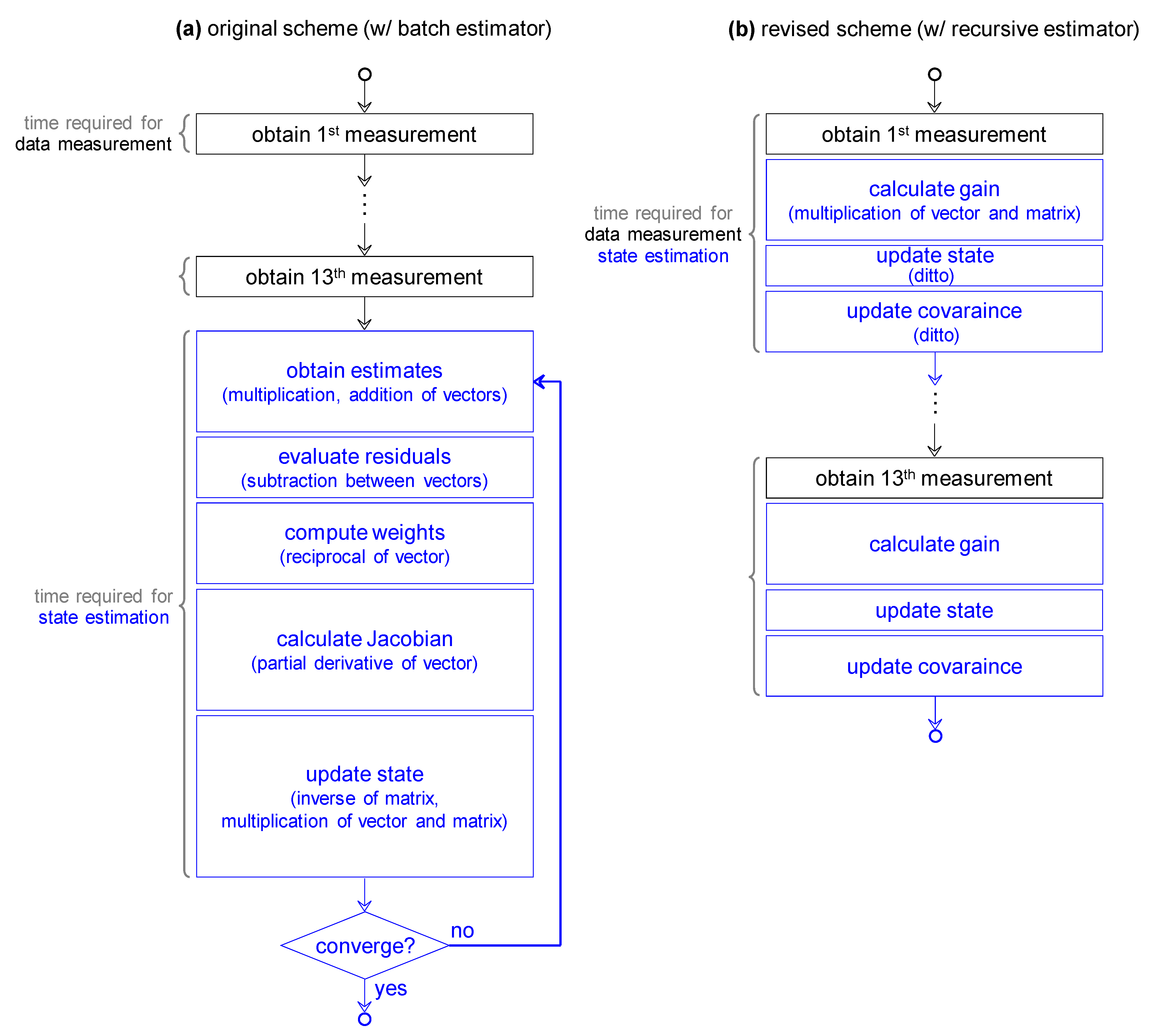
In this study, we improve the original scheme further in another aspect: its state estimator is replaced with recursive least-squares (RLS). For on-line state estimation, a recursive process such as the RLS is typically more favorable than a batch process. The advantages of the RLS are magnified when implemented in BMSs with limited computational resources. In general, matrix inversions are required to solve a cost function. However, it is no longer required for a recursive process. The matrix inversions are CPU intensive operations. Therefore, eliminating them will aid in reducing CPU time. Considering BMS implementation, spreading the CPU utilization, rather than reducing CPU time, is more meaningful. This is because BMSs, particularly for use in BEVs, require hard real-time guarantees. State estimators are commonly composed of data measurement and state estimation. Batch estimators run them in series, whereas recursive estimators do so in parallel. It is apparent that the state estimation will consume significantly longer CPU time than the data measurement. Accordingly, it is challenging for batch estimators to level off CPU utilization, whereas recursive estimators can do it straightforwardly. This is considered a benefit of the RLS, specifically for CPU utilization (see Figure 1). With regard to memory footprint, multiple and long vectors are not necessary for a recursive process. In contrast, a batch process typically requires the vectors of measurements, estimates, residuals, and Jacobian. Specifically for the WLS, the vectors of weights are added to them. As previously stated, different weights need to be applied to each of the data points because they are not equally reliable for the SOH estimation. This requirement could be realized simply by using a forgetting factor in the RLS. Thus, we expect to achieve higher applicability of the SOH estimator to computationally inexpensive BMSs, by means of the RLS.

2. Reviewing the Original Scheme

Before addressing a recursive estimator, we briefly revisit the original scheme based on a batch estimator. In the process of the original scheme, we utilize several types of batch estimators. Thereby, we could estimate the state and parameters of the battery model (see

Table 1. Comparison of batch estimators used in the original scheme.

Type of Estimator	Estimate	Notes
Linear Least-squares	Parameters in the battery model	State (SOH) is measured and provided.
Non-linear Least-Squares	State (SOH) in the battery model	Parameters are estimated and provided.
Weighted Least-Squares	ditto	Each measurement is unequally weighted according to its confidence.

).

2.1. Linear Least-Squares

As presented in Table 1, linear least-squares is applied to estimate parameters in the battery model. In this paper, we will call it ordinary least-squares (OLS) in contrast with weighted least-squares (WLS). As discussed earlier, the original scheme exploits changes in the shape of the charge curve with respect to the SOH. This complex relationship can be captured conveniently with the battery model through metamodeling. A series of reformulations of the charge curve finally yields the battery model in the form of the times elapsed to reach target voltages with respect to the SOH. Accordingly, the battery model is reformulated in the form of a second-degree polynomial as

$$t_k={\displaystyle \sum }_{p=0}^2{a}_{k,p}\times SO{H}^p=a_{k,1}+a_{k,2}\times SOH+a_{k,3}\times SO{H}^2$$

(1)

where the values of the parameters $a_{k,p}$ $\left(k=1–n, p=1–3\right)$ are determined by the corresponding target voltages $V_k$ $\left(k=1–n\right)$. Equation (1) can be expanded as

$$\left(\begin{array}{c}\begin{array}{c}{t}_1\\ t_2\end{array}\\ ⋮\\ t_n\end{array}\right)=\left(\begin{array}{c}\begin{array}{c}{a}_{1,1}\\ a_{2,1}\end{array}\\ ⋮\\ a_{n,1}\end{array}\right)+\left(\begin{array}{c}\begin{array}{c}{a}_{1,2}\\ a_{2,2}\end{array}\\ ⋮\\ a_{n,2}\end{array}\right)\times SOH+\left(\begin{array}{c}\begin{array}{c}{a}_{1,3}\\ a_{2,3}\end{array}\\ ⋮\\ a_{n,3}\end{array}\right)\times SO{H}^2$$

(2)

where $n=13$ as the target voltage increases from 3650 to 3950 mV at 25 mV intervals. For example, the time required to reach the first target voltage $V_1$ (3650 mV) is predicted as $t_1=a_{1,1}+a_{1,2}\times SOH+a_{1,3}\times SO{H}^2$. Hence, the values of the parameters $a_{1,p}$ corresponded to their target voltage $V_1$. Similarly, the time required to reach the final target voltage $V_{13}$ (3950 mV) is $t_{13}=a_{13,1}+a_{13,2}\times SOH+a_{13,3}\times SO{H}^2$. This can be also expressed as

$$t_{13}=\left(\begin{array}{ccc}1& SOH& SO{H}^2\end{array}\right)\left(\begin{array}{c}{a}_{13,1}\\ a_{13,2}\\ a_{13,3}\end{array}\right)$$

(3)

If formally organized, suppose ${\left(a_{k,1},a_{k,2},a_{k,3}\right)}^T=H_k$ is a constant yet unknown parameter vector; $\left(1,SOH,SO{H}^2\right)=\left(x_1,x_2,x_3\right)=x$ is a known state vector; and $t_k=y_k$ is a noisy measurement. As the parameters of the reformulate model are linear, $y$ can be a linear combination of $x$ with the addition of certain measurement noise ν. Accordingly, Equation (3) can be generalized as

$$y_k=x{H}_k+{\nu }_k$$

(4)

This section describes determination of the best estimate ${\tilde{H}}_k$ of $H_k$ by using the linear OLS. Given the state vector $x$, the difference between the measured values and predicted values, namely, the prediction error, is described as

$$ϵ={\displaystyle \sum }_{k=1}^n\left(y_k-x{\tilde{H}}_k\right)$$

(5)

From the perspective of least-squares, the value of ${\tilde{H}}_k$ that minimizes the cost function is obtained by

$$cost\left({\tilde{H}}_k\right)={\mathit{ϵ}}^T\mathit{ϵ}={\displaystyle \sum }_{k=1}^n{\left(y_k-x{\tilde{H}}_k\right)}^2$$

(6)

The minimum of Equation (6) can be determined by setting the derivative of the cost function with respect to ${\tilde{H}}_k$ as zero

$$\frac{\partial cost\left({\tilde{H}}_k\right)}{\partial {\tilde{H}}_k}=-2x^T\left(y_k-x{\tilde{H}}_k\right)=0$$

(7)

The solution of Equation (7) results in a normal equation that enables us to estimate ${\tilde{H}}_k$

$$\left(x^{T}x\right){\tilde{H}}_k={\displaystyle \sum }_{k=1}^n{x}^T{y}_k$$

(8)

Provided $x^{T}x$ is non-singular and invertible, the solution takes the form

$${\tilde{H}}_k={\left(x^{T}x\right)}^{-1}{\displaystyle \sum }_{k=1}^n{x}^T{y}_k$$

(9)

where the measurement $y_k$ is obtained from battery cells at different SOHs ranging from 100 to 70%, which corresponds to the state $x$. As shown in Figures 7 and 10 in [15], the shape of the charge curve is affected by the SOH as well as other operational factors before charging, including the duty cycle, rest time, SOC, and temperature. Thus, the values of the contributing factors other than SOH are carefully selected and fixed while measuring the training data. Thereby, they represent various real-world conditions that LIBs for BEVs undergo (see

Table 2. Test conditions for measuring the training data.

Duty Cycle	Rest Time	SOC	Temperature	C-Rate
FTP	1 min	40%	25 °C	1.45C (equivalent to 50 kW charging)

).

The resulting parameter vector ${\tilde{H}}_k$ by means of the linear OLS is tabulated in

Table 3. Estimated parameters in the battery model.

${\mathit{V}}_{\mathit{k}}$	${\mathit{a}}_{\mathit{k},1}$	${\mathit{a}}_{\mathit{k},2}$	${\mathit{a}}_{\mathit{k},3}$
3650	−1.542	9.934 × 102	1.125
3675	−4.000	1.000 × 103	−1.291 × 10−10
3700	5.430 × 10	8.258 × 102	1.317 × 102
3725	9.359 × 10	6.697 × 102	2.843 × 102
3750	2.111 × 102	2.751 × 102	6.296 × 102
3775	2.278 × 102	1.477 × 102	8.197 × 102
3800	1.612 × 102	2.745 × 102	8.357 × 102
3825	1.311 × 102	3.226 × 102	8.923 × 102
3850	1.013 × 102	3.797 × 102	9.414 × 102
3875	1.086 × 10	6.121 × 102	8.704 × 102
3900	−1.183 × 102	9.740 × 102	7.018 × 102
3925	−2.112 × 102	1.252 × 103	5.789 × 102
3950	−2.848 × 102	1.495 × 103	4.689 × 102

.

2.2. Non-Linear Least-Squares

The parameters in the reformulated model are determined by employing the linear OLS. Thus, our battery model becomes ready for use. Because the battery model is non-linear in its state, i.e., $\mathrm{SOH}$, Equation (1) can be expressed with a non-linear function of $h$ as

$$t_k=h\left(a_{kp}, SOH\right)$$

(10)

The previous section described the determination of the values of the parameters $a_{k,p}$ $\left(k=1–n, p=1–3\right)$ (see Table 3). Because they are determined by the corresponding target voltages $V_k$ $\left(k=1–n\right)$, Equation (10) can be rewritten as

$$t_k=h\left(V_k, SOH\right)$$

(11)

If formally stated, suppose $SOH=\tilde{x}$ is an unknown state; and $t_k=y_k$ is a noisy measurement at the corresponding voltages $V_k$. Equation (11) can be generalized as

$$y_k=h\left(\tilde{x}\right)+{\nu }_k$$

(12)

This section describes our determination of the best estimate $\tilde{x}$ of $x$ by using the non-linear OLS. For such non-linear systems, the normal equation in Equation (9) needs to be modified as

$$∆\tilde{x}={\left(J^{T}J\right)}^{-1}{\displaystyle \sum }_{k=1}^n{J}^T∆y_k$$

(13)

where the state $\tilde{x}$ is estimated by successive approximation, $\tilde{x}=\tilde{x}+∆\tilde{x}$. The Jacobian matrix $J$ in Equation (13) is defined as

$$J=\frac{\partial h\left(\tilde{x}\right)}{\partial \tilde{x}}$$

(14)

where $J$ is in the form of a single column vector because the state $x$ is a scalar value. The measurement $y_k$ in Equation (13) is acquired from battery packs in use for a fleet of BEVs. This is distinct from the training data whose preparation was described in the previous section. Now, we validate the parameterized model and its state estimator, i.e., the non-linear OLS. To achieve this, such noisy measurements are necessary, which will reflect randomly specified real-world conditions. We call it test data, in contrast to the training data. As shown in Figure 12 in [15], our validation concludes that the OLS is not reliable against the test data as it fails to satisfy the requirements, including that of an estimation error less than 3%. This is primarily owing to the measurements with significant noise, which correspond to the shape of the charge curve distorted by the uncontrolled operational factors before charging. It is also illustrated that the early part of the charge curve is more vulnerable to being noisy. This can be interpreted as the early part being less reliable than the later part. In order to provide higher weights to more reliable data points on the later part of the charge curve, we introduce the WLS in the next section.

2.3. Weighted Least-Squares

The battery model is equivalent to Equation (1). However, in this section, we assume the measurements to be unequally reliable. This is reflected in test data. Suppose the noise for each measurement ${\nu }_k$ $\left(k=1–n\right)$ has zero mean and is independent of each other. Then, the covariance matrix for all the measurement noise can be represented as

$$R=E\left(\nu {\nu }^T\right)=diag\left({\sigma }_1^2,{\sigma }_2^2,\cdots ,{\sigma }_n^2\right)$$

(15)

The prediction error is considered as before. Thus, the residual vector is $\mathit{ϵ}={\left({\epsilon }_1,{\epsilon }_2,\cdots ,{\epsilon }_n\right)}^T$. For the WLS, the cost function to be minimized is the summation of squared residuals weighted divided by the error variance:

$$cost\left(\tilde{\mathit{x}}\right)={\mathit{ϵ}}^T{R}^{-1}\mathit{ϵ}=\frac{{ϵ}_1^2}{{\sigma }_1^2}+\frac{{ϵ}_2^2}{{\sigma }_2^2}+\cdots +\frac{{ϵ}_n^2}{{\sigma }_n^2}$$

(16)

At a minimum, the partial derivative of the cost function should vanish, so that

$$\frac{\partial cost\left(\tilde{\mathit{x}}\right)}{\partial \tilde{\mathit{x}}}=-2{\mathit{y}}^T{R}^{-1}H+2{\tilde{\mathit{x}}}^T{H}^T{R}^{-1}H=0$$

(17)

Equation (17) is solved to obtain the normal equation that enables us to estimate the state $\tilde{x}$ against the unequally reliable measurement $y$:

$$\tilde{x}={\left(H^T{R}^{-1}H\right)}^{-1}{H}^T{R}^{-1}y$$

(18)

Replacing $R^{-1}$ with the weight vector $W$ yields

$$\tilde{x}={\left(H^{T}WH\right)}^{-1}{H}^{T}Wy$$

(19)

Again, for similar non-linear systems, the normal equation in Equation (19) is modified as

$$∆\tilde{x}={\left(J^{T}WJ\right)}^{-1}{J}^{T}W∆y$$

(20)

As shown in Figure 12 in [15], our validation concludes that the WLS is reliable against the test data as it is capable of satisfying the requirements including an estimation error less than 3%. By providing more weights to the later part of the charge curve, where the data points are more reliable that those in the early part, the estimation error is reduced by 7.8% point.

3. Problem Statement

With reference to the implementation of the WLS to BMSs, we could identify scope for further improvement. This is motivated primarily by our need for an alternative state estimator that exhibits higher BMS-applicability than the WLS, while being as reliable as the WLS.

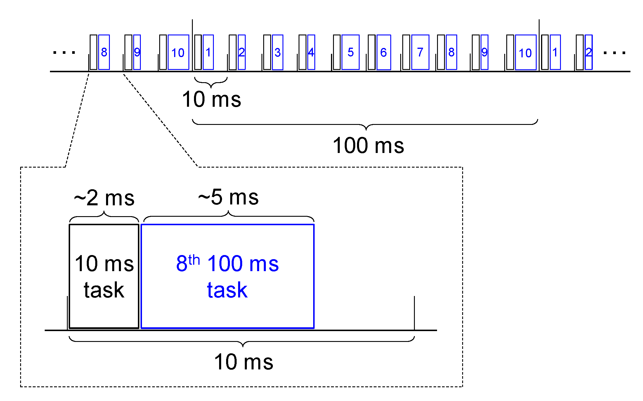
For on-line state estimation, a recursive process tends to be preferred over a batch process. This is true also for SOH estimation. For the BMS, SOH estimation is one of its multiple tasks. Therefore, the implemented SOH estimator is required to run in conjunction with other tasks within a common timeframe. To process multiple tasks using a single-core processor, a scheduler is necessary to decide the task to be executed next. A scheduler in the BMS assigns a timeslot to each task in equal portion and in circular order, thereby processing multiple tasks without priority. We generally call it a round-robin scheduler. A default timeframe common to all the tasks is set to 10 ms. Tasks that need to be executed at higher frequency are assigned at every 10 ms timeslot. The 10 ms tasks primarily include cell monitoring. For example, the voltages from every 96 cells are measured at every 10 ms interval. The current is measured similarly. Such cell monitoring generally consumes less than 2 ms out of the 10 ms timeslot. Tasks that may run at lower frequencies are assigned once every ten 10 ms timeslots. This operates in conjunction with the 100 ms timeslot. The 100 ms tasks involve, for example, battery state estimation. SOH estimation belongs to this category. The SOC and internal resistance are also predicted at every 100 ms interval. Taking into account the relatively slow dynamics of battery states, the 100 ms intervals are considered timely. Within the 10 ms timeslot, the 100 ms tasks are assigned after the 10 ms tasks. This implies that the 100 ms tasks should be performed during the time remaining within the 10 ms timeslot, which is at most approximately 5 ms with a time margin of safety (see Figure 2). If the 100 ms tasks run out of time, the task to be run next lags behind schedule. Thus, a scheduler in the BMS fails to satisfy real-time guarantees. The problem we are concerned with is the vulnerability of batch estimators to this failure.

As previously noted, the implemented SOH estimator comprises two steps: data measurement and state estimation. As SOH estimation is a 100 ms task, the time periods available to each of these is 5 ms. However, the execution times required to complete them are unequal. The data measurement typically consumes approximately 2 ms or less, whereas the state estimation generally uses up the maximum permitted time and occasionally exceeds it. This is mainly because the state estimation incurs longer CPU time than the data measurement does. During the data measurement, the times consumed for reaching the target voltages are measured and then stored in the measurement vector. In contrast, the state estimation is supposed to address computationally denser tasks in the provided time. During the state estimation, the times required to reach the target voltages are first predicted from the battery model and then stored in the estimate vector. The residual vector is produced by subtracting the estimate vector from the measurement vector. Next, the weight vector is produced by taking the reciprocal of the residual vector. Then, the Jacobian, the partial derivative of the residual vector, is numerically calculated. With the calculated Jacobian, the state is updated iteratively until it converges. As a consequence, the execution time required for the state estimation is significantly longer and more uncertain than that required for the data measurement. This is more likely to break real-time guarantees.

This potential albeit critical problem could be addressed by applying a recursive estimator to on-line state estimation. In the following section, we introduce recursive least-squares (RLS) that aids in spreading the computational costs across consecutive timeslots, which is crucial to the BMS implementation.

4. Introducing the Revised Scheme

Similar to the original scheme, the revised scheme captures the shape of the charge curve varying with the SOH. However, rather than the batch estimators, a recursive estimator is employed, expecting its higher applicability to on-line monitoring of the SOH. Suppose we estimate a state ${\tilde{x}}_{k-1}$ after $k-1$ measurements and then obtain a new measurement $y_k$. Using the RLS, we update ${\tilde{x}}_{k-1}$ to ${\tilde{x}}_k$ without requiring the solving of the normal equation in Equations (9) or (20), which is computationally intensive.

We first observe the final form of the RLS:

$${\tilde{x}}_k={\tilde{x}}_{k-1}+K_k\left(y_k-{\tilde{x}}_{k-1}{H}_k\right)$$

(21)

where the gain vector $K_k$ corrects the previous state ${\tilde{x}}_{k-1}$ with the one-step-ahead prediction error $y_k-{\tilde{x}}_{k-1}{H}_k$. That is, the new state ${\tilde{x}}_k$ is corrected from the previous state ${\tilde{x}}_{k-1}$ by the gain vector $K_k$. With the aim of deriving Equation (21), the normal equation in the previous section is rewritten in the recursive context, so that

$$\left({\displaystyle \sum }_{k=1}^n{H}_k{H}_k^T\right){\tilde{x}}_k={\displaystyle \sum }_{k=1}^n{H}_k{y}_k$$

(22)

Provided that ${\displaystyle \sum }{H}_k{H}_k^T$ is non-singular and invertible, the solution takes the following form:

$${\tilde{x}}_k={\left({\displaystyle \sum }_{k=1}^n{H}_k{H}_k^T\right)}^{-1}{\displaystyle \sum }_{k=1}^n{H}_k{y}_k$$

(23)

Reformulating with $P_k$ and $b_k$ yields

$${\tilde{x}}_k=P_k{b}_k$$

(24)

where $P_k={\left({\displaystyle \sum }{H}_k{H}_k^T\right)}^{-1}$ and $b_k={\displaystyle \sum }{H}_k{y}_k$. In the recursive perspective, $P_k$ and $b_k$ can be described with the previous $P_{k-1}$ and $b_{k-1}$, respectively:

$$P_k^{-1}=P_{k-1}^{-1}+H_k{H}_k^T$$

(25)

$$b_k=b_{k-1}+H_k{y}_k$$

(26)

Equation (25) is rearranged as

$$P_{k-1}=P_k+P_k{x}_k{x}_k^T{P}_{k-1}$$

(27)

Then, multiplying by $x_k$ yields

$$P_{k-1}{x}_k=P_k{x}_k\left(1+x_k^T{P}_{k-1}{x}_k\right)$$

(28)

Multiplying this by ${\left(1+x_k^T{P}_{k-1}{x}_k\right)}^{-1}{x}_k^T{P}_{k-1}$ yields

$$P_{k-1}{x}_k{\left(1+x_k^T{P}_{k-1}{x}_k\right)}^{-1}{x}_k^T{P}_{k-1}=P_k{x}_k{x}_k^T{P}_{k-1}$$

(29)

Substituting Equations (27), (29) is formulated as

$$P_k=P_{k-1}-P_{k-1}{x}_k{\left(1+x_k^T{P}_{k-1}{x}_k\right)}^{-1}{x}_k^T{P}_{k-1}$$

(30)

Now, substituting Equations (26) and (30) into Equation (24) yields

$${\tilde{x}}_k=\left\{P_{k-1}-P_{k-1}{x}_k{\left(1+x_k^T{P}_{k-1}{x}_k\right)}^{-1}{x}_k^T{P}_{k-1}\right\}\left\{b_{k-1}+H_k{y}_k\right\}$$

(31)

Noting that $x_{k-1}=P_{k-1}{b}_{k-1}$, Equation (31) can be expanded to yield

$${\tilde{x}}_k={\tilde{x}}_{k-1}+K_k\left(y_k-{\tilde{x}}_{k-1}{H}_k\right)$$

(32)

with the gain vector

$$K_k=P_{k-1}{x}_k{\left(1+x_k^T{P}_{k-1}{x}_k\right)}^{-1}$$

(33)

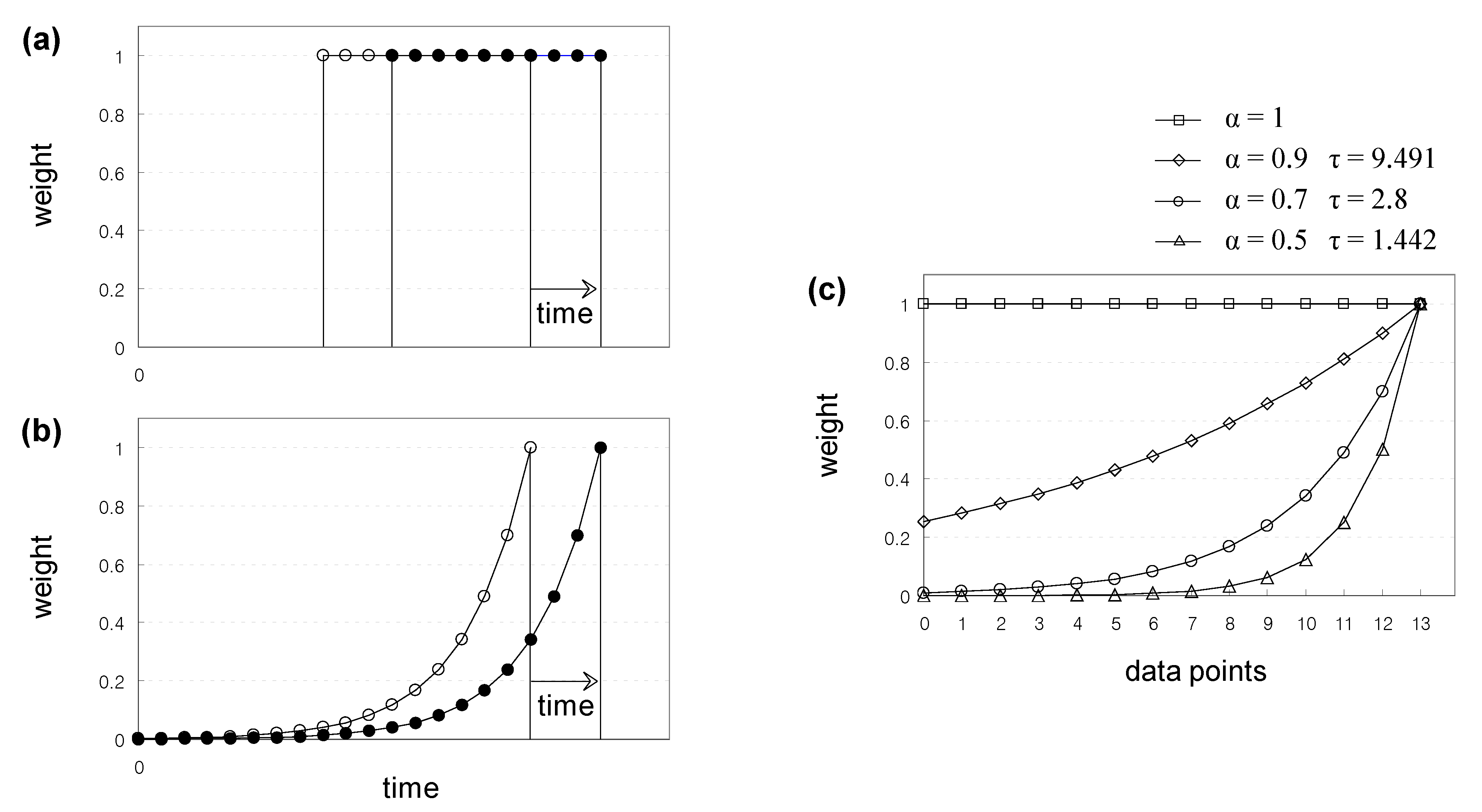
As the WLS mitigates the effect of obsolete measurements on the state estimation, the RLS is also expected to do so. As aforementioned, this is mainly related to the fact that not all measurements are equally reliable. The early part of the charge curve is subject to being noisier than the later part because it is more exposed to the effect of the operational factors before charging. For recursive estimators, there are generally two options to provide higher weights to more reliable data points. One is commonly called a moving rectangular window, and the other is an exponentially weighted window (see Figure 3a,b). The second option is selected in this work as it functions more similarly to the WLS. As its name indicates, the exponentially weighted window can provide progressively higher weights to the more current data points. Thereby, it causes the state estimation to be more sensitive to recent changes in the shape of the charge curve. By applying an exponential forgetting factor $\alpha$, the gain vector $K_k$ in Equation (33) is modified as

$$K_k=P_{k-1}{x}_k{\left(\alpha +x_k^T{P}_{k-1}{x}_k\right)}^{-1}$$

(34)

with the covariance matrix

$$P_k=\frac{1}{\alpha }\left(P_{k-1}-K_k{x}_k^T{P}_{k-1}\right)$$

(35)

In Equations (34) and (35), $\alpha$ is relevant to a decay time constant $\tau$ by

$$\alpha =exp\left(-\frac{∆t}{\tau }\right)$$

(36)

where $∆t$ is a time interval within data points (see Figure 3c). A more detailed description of RLS is available in [18].

5. Experimental Validation of the Revised Scheme

In this section, we describe the experimental validation of the revised scheme from two aspects. One is from the perspective of BMSs. It addresses, for example, the CPU time and memory footprint required to implement the recursive estimator. The other is from the batteries’ perspective. It addresses the accuracy of the SOH estimation by using the recursive estimator. Each of these performance metrics of the recursive estimator is compared to those of the batch estimator such that the revised scheme could be evaluated in comprehensive and quantitative terms.

Prior to assessing the revised scheme, we briefly introduce the hardware specification of the BMS used in this work. As described in [15], the previous BMS is not equipped with the floating-point unit (FPU), which is specifically designed to perform floating-point arithmetic. It is established that the RLS exhibits finite precision effects, which causes it to become numerically unstable and eventually fail to converge. In order to run the RLS in a fast, effective, and reliable manner, an FPU-equipped BMS is newly deployed in this work (see

Table 4. Comparison of BMS hardware specification.

	Previous	New
Model	XC2387	TC264D
CPU	16 bit, 80 MHz, without FPU	32 bit, 200 MHz, with FPU
RAM, ROM	82 kB, 768 kB	240 kB, 2.5 MB

).

5.1. BMS Implementation

With the introduction of the RLS, the process of the revised scheme comprises of the iteration of the data measurement, and the state estimation. Before the first measurement $\left(k=0\right)$, we have certain prior information about the state. This becomes our initial state. If we do not have the prior SOH, the initial SOH is set as one. Although this is an unfavorable condition to the SOH estimator, it could occur if the prior SOH stored in a BMS is unavailable, e.g., owing to the battery or its BMS replacement. There is some uncertainty of the initial state. This becomes our initial covariance. The initial covariance is set close to zero, i.e., 1e-4. After the first measurement $\left(k=1\right)$, we sequentially update the state and its error covariance according to (32–35). As noted before, the target voltages are predetermined as 3650–3950 mV at intervals of 25 mV. Thereby, 13 data points are produced. Hence, after the 13th measurement $\left(k=13\right)$, we finalize this update. In order to impose higher weights upon the more recent measurements, a forgetting factor of 0.7 is selected and applied. With these hyper-parameters, the recursive estimator is implemented to the BMS.

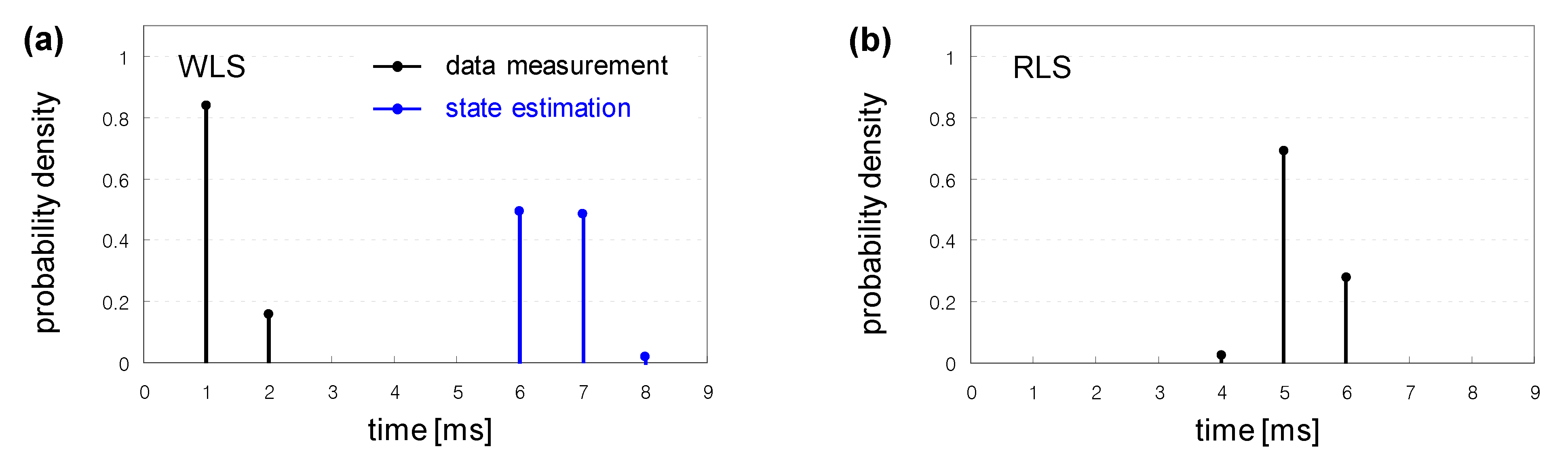
It is observed that the implemented recursive estimator is capable of spreading CPU time across consecutive timeslots while guaranteeing real-time execution of tasks (see Figure 4). The recursive estimator exhibits a largely even execution time in the order of 5 ms. In contrast, the batch estimator exhibits a varying execution time ranging from 1 to 8 ms. This is related mainly to its two steps. The data measurement consumes less than 2 ms, whereas the state estimation requires 6–7 ms. It is also observed that the implemented recursive estimator can reduce the memory footprint by over 60%. The batch estimator primarily carries eight long vectors. They include the vectors of measurements, estimates, residuals, weights, and Jacobian. They also include the three parameter vectors. Their column size is 13. Each vector thus consumes 104 bytes (8 bytes × 13 floating-point numbers). Moreover, overall, 832 bytes of RAM are always required during run-time. In contrast, the recursive estimator uses only the three parameter vectors. Thus, only 312 bytes of RAM are occupied. It is observed that this comparison considers only such long vectors that require relatively large arrays. Considering the uniform CPU time and the low memory usage, it is concluded that a recursive process is more readily applicable to the BMS than a batch process is.

5.2. SOH Estimation

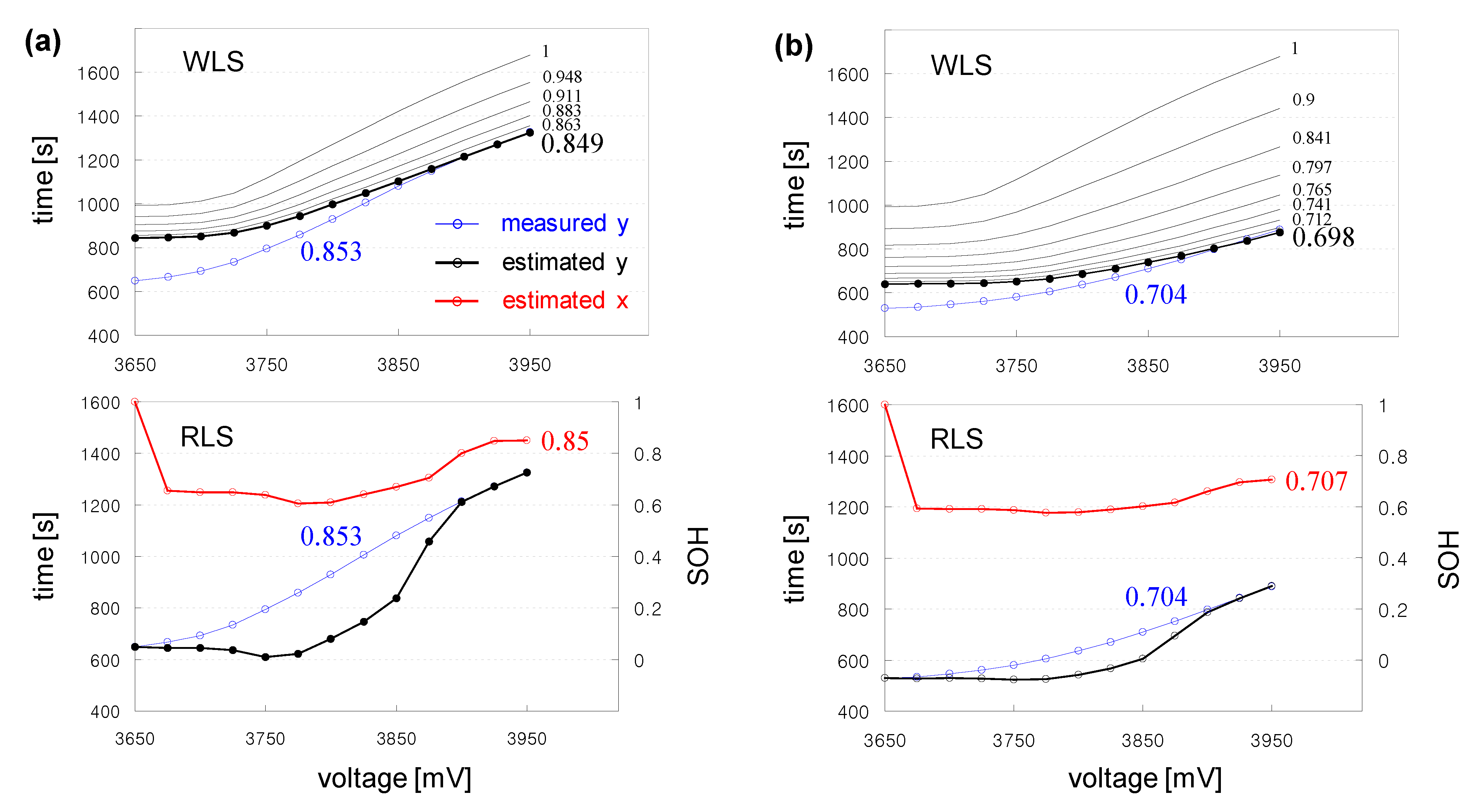
The test data sets are consistent with those provided in the original work. Two battery packs in use for a fleet of BEVs are employed to provide the test data. Their present capacities are first measured under the standard conditions. The values obtained are 35.8 Ah and 29.6 Ah, respectively. Each of them has a nominal capacity of 42 Ah. Thus, their SOHs are 85.3% and 70.4%, respectively. It is observed that the SOH of the entire pack is determined by the cell that has the least capacity and generally exhibits the largest internal resistance. Then, their present capacities are estimated under randomly specified real-world conditions. With respect to the test data, it is observed that the recursive estimator is as reliable as the batch estimator (see Figure 5); the difference between the two estimators is less than 1%. The difference between the estimate from the recursive estimator and the measurement is also within 1%.

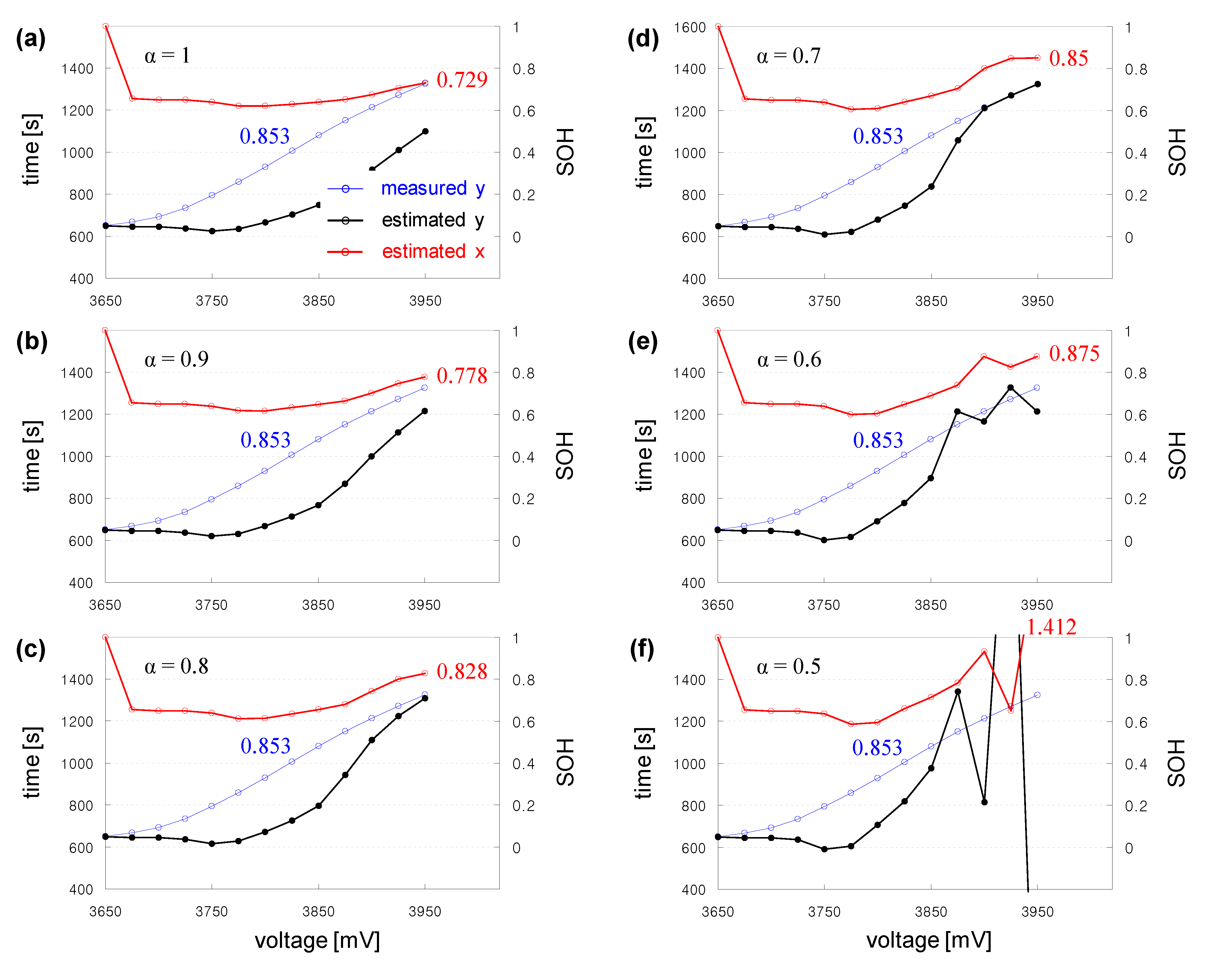
These results are from the recursive estimator for implementation with hyper-parameters, including a forgetting factor of 0.7. In general, the forgetting factor affects two conflicting properties of a recursive estimator: tracking and convergence. The selection of an effective value for the forgetting factor is thus based on a trade-off between these. It is observed that as the forgetting factor reduces to 0.7, better tracking is achieved (see Figure 6a–d). In contrast, as the forgetting factor decreases below 0.7, lower convergence is observed (see Figure 6e,f). This illustrates that specifically for our problem, a forgetting factor of 0.7 is optimal in that it will aid the RLS in straightforwardly adapting to recent measurements, while preventing the RLS from becoming too sensitive to measurement noise.

6. Conclusions

In this work, the original scheme based on a batch process is revised, considering its BMS implementation. The original scheme uses the WLS, which requires Jacobian calculation and matrix inversion to solve the normal equation. Therefore, in a batch process, state estimation requires significantly more intensive CPU utilization and larger memory footprint than those for data measurement. This is detrimental to its BMS implementation. By replacing a batch process to solve the normal equation with a recursive update, the revised scheme aids in spreading CPU utilization. The revised scheme also aids in reducing memory footprint because it does not require long and multiple vectors to formulate the normal equation. The advantage of the revised scheme is quantitatively validated against the test data. It is observed that the recursive estimator spends largely uniform execution time in the order of 5 ms. This is in contrast to the batch estimator, which exhibits varying execution time ranging from 1 to 8 ms. Furthermore, it is observed that the recursive estimator occupies more than 60% less memory footprint than the batch estimator does. Notwithstanding such substantial revisions made to the state estimator, a similar level of accuracy of SOH estimation is attained.

References

- 2018 Nissan Leaf Battery Specification. Available online: https://pushevs.com/2018/01/29/2018-nissan-leaf-battery-real-specs/ (accessed on 1 March 2019).
- Verbrugge, M.; Koch, B. Generalized recursive algorithm for adaptive multiparameter regression application to lead acid, nickel metal hydride, and lithium-ion batteries. J. Electrochem. Soc. 2006, 153, A187–A201. [Google Scholar] [CrossRef]
- Guo, Z.; Qiu, X.; Hou, G.; Liaw, B.Y.; Zhang, C. State of health estimation for lithium ion batteries based on charging curves. J. Power Sources 2014, 249, 457–462. [Google Scholar] [CrossRef]
- Eddahech, A.; Briat, O.; Vinassa, J.M. Determination of lithium-ion battery state-of-health based on constant-voltage charge phase. J. Power Sources 2014, 258, 218–227. [Google Scholar] [CrossRef]
- Roscher, M.A.; Assfalg, J.; Bohlen, O.S. Detection of utilizable capacity deterioration in battery systems. IEEE Trans. Veh. Technol. 2010, 60, 98–103. [Google Scholar] [CrossRef]
- Kessels, J.T.B.A.; Rosca, B.; Bergveld, H.J.; Van Den Bosch, P.P.J. On-line battery identification for electric driving range prediction. In Proceedings of the 2011 IEEE Vehicle Power and Propulsion Conference, Chicago, IL, USA, 6–9 September 2011. [Google Scholar]
- Kim, I.S. A technique for estimating the state of health of lithium batteries through a dual-sliding-mode observer. IEEE Trans. Power Electron. 2009, 25, 1013–1022. [Google Scholar]
- Plett, G.L. Recursive approximate weighted total least squares estimation of battery cell total capacity. J. Power Sources 2011, 196, 2319–2331. [Google Scholar] [CrossRef]
- Andre, D.; Appel, C.; Soczka-Guth, T.; Sauer, D.U. Advanced mathematical methods of SOC and SOH estimation for lithium-ion batteries. J. Power Sources 2013, 224, 20–27. [Google Scholar] [CrossRef]
- Remmlinger, J.; Buchholz, M.; Soczka-Guth, T.; Dietmayer, K. On-board state-of-health monitoring of lithium-ion batteries using linear parameter-varying models. J. Power Sources 2013, 239, 689–695. [Google Scholar] [CrossRef]
- Schwunk, S.; Armbruster, N.; Straub, S.; Kehl, J.; Vetter, M. Particle filter for state of charge and state of health estimation for lithium–iron phosphate batteries. J. Power Sources 2013, 239, 705–710. [Google Scholar] [CrossRef]
- Schmidt, A.P.; Bitzer, M.; Imre, Á.W.; Guzzella, L. Model-based distinction and quantification of capacity loss and rate capability fade in Li-ion batteries. J. Power Sources 2010, 195, 7634–7638. [Google Scholar] [CrossRef]
- Prasad, G.K.; Rahn, C.D. Model based identification of aging parameters in lithium ion batteries. J. Power Sources 2013, 232, 79–85. [Google Scholar] [CrossRef]
- Can you Recycle or Re-Use EV Batteries? Available online: https://pushevs.com/2018/01/29/2018-nissan-leaf-battery-real-specs/ (accessed on 15 May 2019).
- Sung, W.; Nam, J.; Choi, J.H.; Lee, J. Robust and efficient capacity estimation using data-driven metamodel applicable to battery management system of electric vehicles. J. Electrochem. Soc. 2016, 163, A981–A991. [Google Scholar] [CrossRef]
- Sung, W.; Lee, J. Improved capacity estimation technique for the battery management systems of electric vehicles using the fixed-point iteration method. Comput. Chem. Eng. 2018, 117, 283–290. [Google Scholar] [CrossRef]
- Lee, J.; Sung, W.; Choi, J.H. Metamodel for efficient estimation of capacity-fade uncertainty in Li-Ion batteries for electric vehicles. Energies 2015, 8, 5538–5554. [Google Scholar] [CrossRef]
- Young, P.C. Chapter 3 Recursive Least Squares Estimation. In Recursive Estimation and Time-Series Analysis: An Introduction for the Student and Practitioner, 2nd ed.; Springer Science & Business Media: Berlin/Heidelberg, Germany, 2011; pp. 29–32. [Google Scholar]
© 2019 by the authors. Licensee MDPI, Basel, Switzerland. This article is an open access article distributed under the terms and conditions of the Creative Commons Attribution (CC BY) license (http://creativecommons.org/licenses/by/4.0/).