Modified Technique of Parameter Identification of a Permanent Magnet Synchronous Motor with PWM Inverter in the Presence of Dead-Time Effect and Measurement Noise

Abstract

The paper considers the problem of parameter identification of the surface mounted permanent magnet synchronous motor (SPMSM) with pulse width modulated (PWM) inverter in the presence of dead time of power switches and other nonlinear distortions. Parameter identification of the SPMSM is required for the tuning of the torque control loop, because in some cases, the exact values of phase resistances and inductances are not known. In the absence of nonlinear disturbances, the problem of SPMSM parameters estimation is not difficult. The influence of the dead-time effect, back electromotive force and measurements noise introduces distortions in experimental output data sets, which leads to incorrect parameter estimation. Thus, there is a need to develop new designs of identification experiments and methods of processing of the experimental data. A detailed mathematical model of SPMSM with a PWM inverter in the presence of dead-time effect is considered in the paper. The negative influence of the dead-time effect on the results of parameter estimation is shown. A modified technique of parameter identification of SPMSM based on the estimation of frequency response function is proposed. The applied design of identification experiments, the type of excitation input signal, and methods of data processing allow us to minimize the influence of nonlinear disturbances and to reduce the variance of estimation of frequency response function. These features provide a high performance of SPMSM parameters estimation.

1. Introduction

Permanent magnet synchronous motors (PMSM) are widely used in adjustable-speed electric drives. One of the important applications of the PMSM are high-precision direct drive servo systems. The advantages and disadvantages of using the PMSM in such systems are described in many scientific works, for example [1,2,3,4,5]. Effective torque control of the PMSM under different operating conditions remains an important scientific task [6,7,8,9].

Different strategies and approaches to the synthesis of the current (torque) control loop for the PMSM have been developed and researched. A classic and quite effective solution is the use of a linear or modified proportional–integral controller [8,10,11,12]. The most known techniques for tuning the current (torque) control loop require knowledge of the electrical parameters of the PMSM, particularly the phase resistances and inductances. However, in many practical cases the electrical parameters of the PMSM can be unknown. The paper is devoted to the problem of identification of electrical parameters of the surface mounted PMSM (SPMSM) in the presence of distortions associated with the nonlinearity of the power converter.

Control of the PMSM is provided by the DC-AC semiconductor converter with pulse width modulation (PWM). Field-effect transistors or insulated gate bipolar transistors (IGBT) are used as switching devices. These devices have finite switching times, so engineers introduce a delay in the switching of transistors which are installed in the same phase. This delay, called dead time, is necessary to prevent the simultaneous switching on of two transistors in the same phase of the PWM inverter, resulting in a short circuit in the phase. During the dead time, the voltage in the corresponding phase is determined by the direction of current [13,14]. Dead-time and voltage drops across the switching devices cause distortions of the inverter’s output voltage, which are called the dead time effect.

Distortion of the inverter output voltages leads to distortion of phase currents of the PMSM and the appearance of torque ripples. Main approaches which are used to reduce the negative effects caused by the dead time effect are follows:

• change of the PWM inverter design or switch control algorithms [15,16];
• application of modified control algorithms to reduce torque ripples, including repetitive, iterative-learning or self-tuning controllers [17,18,19];
• compensation of the dead-time effect using its mathematical models [14,20,21,22].

The problem of the parameter identification of the PMSM is quite widely described in the scientific literature, for example [23,24,25,26,27]. In most cases, numerical estimation models such as ARX (autoregressive extra input), ARMA (autoregressive moving average), OE (output error) and others based on experimental data in the time domain are used to estimate parameters of the SPMSM. Experimental parameter identification of the PMSM is complicated by the influence of distortions such as torque ripples, back electromotive force (back emf) and cross-coupling of currents in the dq coordinate model. There are effective techniques of parameter identification that take into account the influence of back emf and the cross-coupling of currents [23,25,28]. Modified numerical estimation algorithms are proposed in [26,29].

However, the influence of the dead time effect on identification results is not considered in most works [13,22]. In the previous paper [13], part of the author’s team in this paper proposed a new method of parameter identification based on the use of modified mathematical model of the SPMSM with a PWM inverter in the presence of the dead time effect.

The parameters of the transfer function can also be obtained from the experimental frequency response function (FRF) [30,31]. For this purpose, different graphical and numerical estimation methods [31,32,33,34,35,36] can be used. Parameter estimation by FRF is performed on much smaller data sets than in the case of time series, which reduces the operating time of algorithms and in many cases provides better accuracy of estimation [33,35,37].

The use of noisy or distorted data sets to estimate structure and parameters of the transfer functions can lead to big variance of the estimated FRF and incorrect parameter estimation results. To reduce the variance of estimated FRF, various methods of spectral analysis can be used, such as the modified Welch periodogram method [31,38], the Blackman–Tukey method [39], and the transient response estimation [33].

In addition, there are the zero-order hold effect, and computational and measurement delays in the digital control system of the PMSM. The delay value is usually assumed to be equal to one or two sampling periods of the control system [40]. The presence of delay should be considered during identification in time domain and does not affect the identification in the frequency domain. The effect of zero order hold leads to distortions of the transfer coefficient at high frequencies close to the Nyquist frequency, which should be considered during identification in the frequency domain [40,41].

This paper proposes a more generalized approach to solving this problem, which does not require the use of complex analytical models of numerical parameter estimation and is based on the estimation of the experimental FRF of the PMSM with PWM inverter. The paper deals with high-precision servo drive systems equipped with rotor position sensors (encoders).

Our paper is organized as follows: In Section 2, the mathematical model of the SPMSM with the PWM inverter in the presence of the dead time effect is described. In Section 3, the negative influence of dead time on the results of parameter identification of the SPMSM is shown. In Section 4, a modified technique of parameter identification of the SPMSM is proposed, the choice of the experiment design, the excitation input signal and the method of data processing are described. The discussion and conclusions are presented in Section 5. All numerical examples given in the paper were implemented in MATLAB 2015a.

2. Mathematical Model of a SPMSM with a PWM Inverter

2.1. Mathematical Model of a SPMSM with an Ideal PWM Inverter

The system of differential equations for phase currents that describes the mathematical model of three-phase SPMSM with the PWM inverter can be written as follows [13]:

$$\{\begin{array}{l}\left(R_a+L_a\frac{d}{dt}\right)i_a(t)=u_0(t)\cdot K_U\cdot \sin (p\alpha (t))+e_a(t),\\ \left(R_b+L_b\frac{d}{dt}\right)i_b(t)=u_0(t)\cdot K_U\cdot \sin (p\alpha (t)-\frac{2\pi }{3})+e_b(t),\\ \left(R_c+L_c\frac{d}{dt}\right)i_c(t)=u_0(t)\cdot K_U\cdot \sin (p\alpha (t)+\frac{2\pi }{3})+e_c(t),\\ M(t)=-\frac{(e_a(t)i_a(t)+e_b(t)i_b(t)+e_c(t)i_c(t))}{\omega (t)},\end{array}$$

(1)

where R_a, R_b, R_c are phases electrical resistances of three-phase SPMSM; L_a, L_b, L_c are phases inductances of three-phase SPMSM; e_a(t), e_b(t), e_c(t) are back emfs which are induced in the phases of SPMSM during the rotation, u₀(t) is the generalized control signal, which is changed in the range [–1; 1], $\omega (t)$ is the angular velocity of the SPMSM; $\alpha (t)$ is the angle of rotation of the SPMSM, K_U = U_DC/2 in case of sinusoidal PWM, and K_U = U_DC/√3 in case of sinusoidal PWM with third harmonic injection or space vector PWM. If windings of the stator are close to a symmetric and balanced three-phase system, the difference between electrical resistances and inductances in the SPMSM phases can be neglected: R_a = R_b = R_c = R and L_a = L_b = L_c = L.

If the currents in the phases of the SPMSM and corresponding back emfs have the following sinusoidal forms:

$$\{\begin{array}{l}{i}_a(t)=I_m\sin (p\alpha (t)+\psi ),\\ i_b(t)=I_m\sin (p\alpha (t)+\psi +\frac{2\pi }{3}),\\ i_c(t)=I_m\sin (p\alpha (t)+\psi -\frac{2\pi }{3}),\end{array} \{\begin{array}{l}{e}_a(t)=-c_e\omega (t)\sin (p\alpha (t)),\\ e_b(t)=-c_e\omega (t)\sin (p\alpha (t)+\frac{2\pi }{3}),\\ e_c(t)=-c_e\omega (t)\sin (p\alpha (t)-\frac{2\pi }{3}),\end{array}$$

(2)

the torque M(t) will not depend on the angle of rotation of the SPMSM:

$$M(t)=1.5c_e{I}_m\cos (\psi ),$$

(3)

where c_e is the back emf constant, and ψ is the angle between the rotor’s angular position and the actual position of the rotor’s magnetic axis. The desired value of the torque M(t) can be achieved by varying the values of I_m and ψ. The maximum torque per ampere is reached when ψ = 0, and the torque is equal to zero when ψ = ±π/2.

Typically, in electric drives, the torque M(t) is not directly measured. However, the measured phase currents i_a(t) i_b(t) i_c(t) can be used to estimate M(t). Here we introduce the term for the generalized current i₀(t) that is calculated as follows:

$$i_0(t)=\frac{2}{3}\left(i_a(t)\sin (p\alpha (t))+i_b(t)\sin (p\alpha (t)+\frac{2\pi }{3})+i_c(t)\sin (p\alpha (t)-\frac{2\pi }{3})\right).$$

(4)

Then Equation (3) for the torque M(t) takes the following form:

$$M(t)=1.5c_e{i}_0(t),$$

From Equations (1), (2) and (4), the following differential equation for the generalized current i₀(t) can be obtained:

$$T_e\frac{d(i_0(t))}{dt}+i_0(t)=\frac{1}{R}\left(K_U{u}_0(t)-c_e\omega (t)\right)-T_{e}p\omega (t)\cdot I_m\sin (\psi ),$$

where T_e is the electrical time constant of the SPMSM.

The mathematical model of three-phase SPMSM with PWM inverter in dq coordinate system has the following form [10]:

$$\{\begin{array}{l}\left(1+T_e\frac{d}{dt}\right)i_d(t)=\frac{K_U}{R}{u}_d(t)+T_{e}p\omega (t)i_q(t),\\ \left(1+T_e\frac{d}{dt}\right)i_q(t)=\frac{K_U}{R}{u}_q(t)-T_{e}p\omega (t)i_d(t)-\frac{c_e\omega (t)}{R},\\ M(t)=1.5c_e{i}_q(t),\end{array}$$

where u_d(t) and u_q(t) are control signals for d and q components, which are changed in the range [–1; 1], currents i_d(t) and i_q(t) are expressed as follows:

$$\{\begin{array}{l}{i}_d(t)=\frac{2}{\sqrt{3}}\left(i_a(t)\sin (p\alpha (t)+\frac{\pi }{3})+i_b(t)\sin (p\alpha (t))\right),\\ i_q(t)=\frac{2}{\sqrt{3}}\left(i_a(t)\cos (p\alpha (t)+\frac{\pi }{3})+i_b(t)\cos (p\alpha (t))\right).\end{array}$$

In this case, phase voltages of the SPMSM can be expressed using u_d(t) and u_q(t) as follows:

$$\{\begin{array}{l}{u}_a(t)=K_U\left(u_d(t)\cos (p\alpha (t))-u_q(t)\sin (p\alpha (t))\right),\\ u_b(t)=K_U\left(u_d(t)\cos (p\alpha (t)-\frac{2\pi }{3})-u_q(t)\sin (p\alpha (t)-\frac{2\pi }{3})\right),\\ u_c(t)=-(u_a(t)+u_b(t)).\end{array}$$

If the stator phase currents of the SPMSM correspond to Equation (2), currents i_d(t) and i_q(t) are expressed as follows:

$$\{\begin{array}{l}{i}_d=I_m\sin \psi \\ i_q=I_m\cos \psi \end{array}$$

The desired value of the torque M(t) can be achieved varying the values of I_m and ψ, which is similar to the mathematical model of the SPMSM for phase currents.

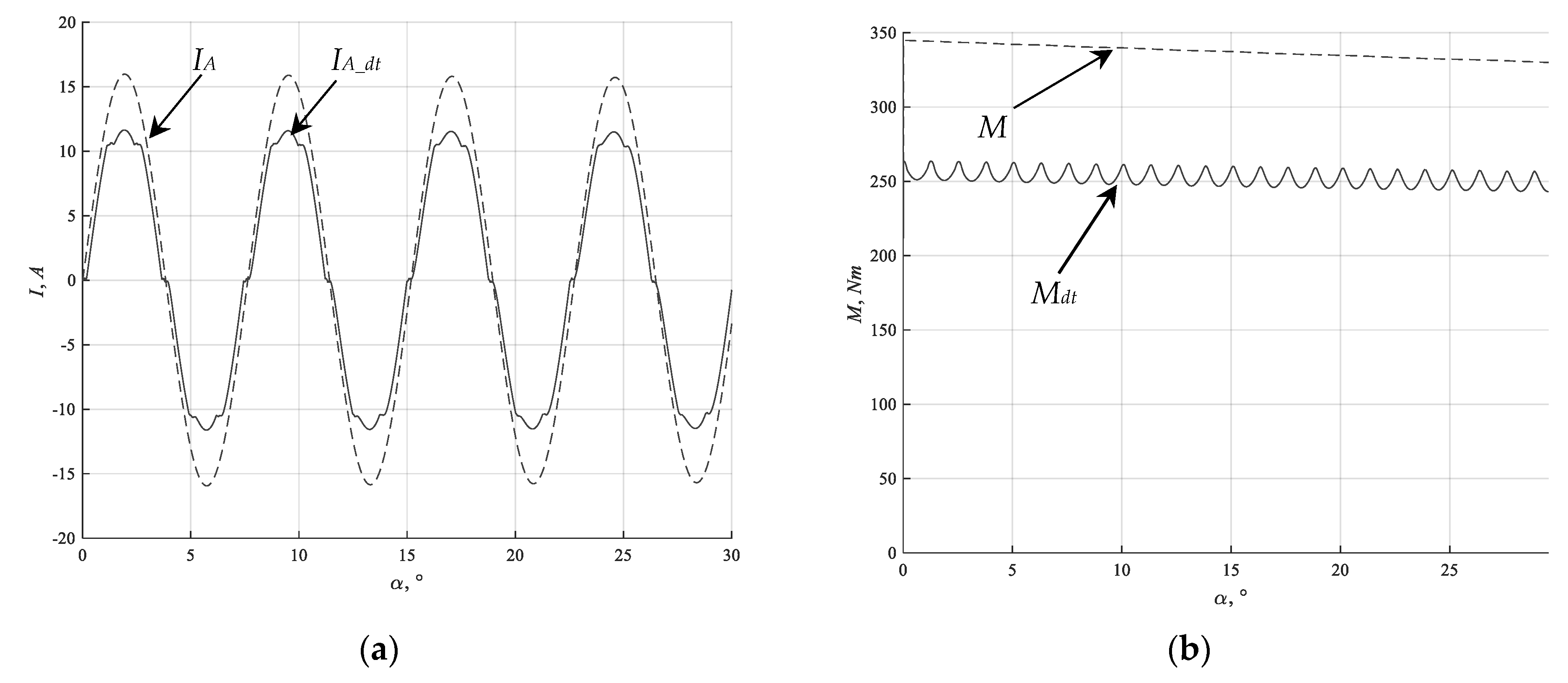
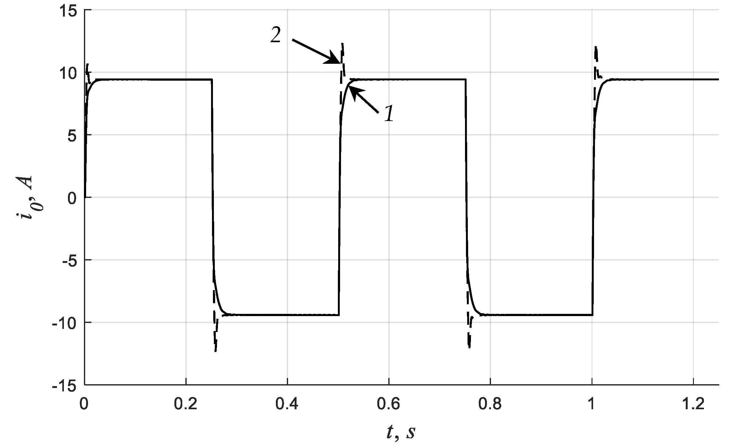
2.2. Mathematical Model of a SPMSM with PWM Inverter in the Presence of the Dead-Time Effect.

The relative switch-on delay τ is defined as the ratio of dead time t_dead to PWM switching time T_sw:

$$\tau =\frac{t_{dead}}{T_{sw}}$$

During the dead time, the phase voltage is determined by the direction of the current as shown in Figure 1. The output voltage of the inverter’s phase is also distorted by the voltage drop across the switching devices. When the difference between the voltage drop across the switching devices in the positive and negative directions of current can be neglected, the phase’s electric potential, can be written as follows:

$${\phi }_{av}=\left({\gamma }_h-\frac{1}{2}-\tau \cdot sign(i)\right)U_{DC}-\Delta u_{const}sign(i).$$

where i is the current in the corresponding phase of the SPMSM, Δu_const is the voltage drop across the switching devices.

Phase voltage distortions of the PWM inverter caused by dead-time effect and voltage drop across the switching devices can be expressed as follows:

$$\begin{array}{l}\Delta U_a(t)=\left(\Delta u_{const}+\tau U_{DC}\right)sign(i_a(t)), \\ \Delta U_b(t)=\left(\Delta u_{const}+\tau U_{DC}\right)sign(i_b(t)),\\ \Delta U_c(t)=\left(\Delta u_{const}+\tau U_{DC}\right)sign(i_c(t)).\end{array}$$

The system of equations for the SPMSM phase currents in the presence of dead time can be written as follows [13]:

$$\{\begin{array}{l}\left({\phi }_{а}(t)-\Delta U_a(t)\right)-\left({\phi }_{с}(t)-\Delta U_c(t)\right)=\\ =(2i_a(t)+i_b(t))R-(e_a(t)-e_c(t))+L\frac{d(2i_a(t)+i_b(t))}{dt},\\ \left({\phi }_b(t)-\Delta U_b(t)\right)-\left({\phi }_{с}(t)-\Delta U_c(t)\right)=\\ =(2i_b(t)+i_a(t))R-(e_b(t)-e_c(t))+L\frac{d(2i_b(t)+i_a(t))}{dt},\\ i_a(t)+i_b(t)+i_c(t)=0,\end{array}$$

(5)

where φ_a, φ_b, φ_c are average electric potentials of the phases of PWM inverter for the period of switching.

An example of phase current distortion and SPMSM torque distortion caused by the dead-time effect is shown in Figure 2.

In the case when sinusoidal PWM, with a third harmonic injection is used, the differential equation for the generalized current i₀(t), in the presence of the dead-time effect and voltage drop on the power switches, is expressed as follows:

$$T_e\frac{d(i_0(t))}{dt}+i_0(t)=\frac{U_{DC}-2u_{const}}{\sqrt{3}R}{u}_0(t)-\frac{c_e\omega (t)}{R}-f_{inv}(t),$$

(6)

where the disturbance function f_inv(t) has the followed form:

$$\begin{array}{l}{f}_{inv}(t)=\frac{1}{R}(\frac{2}{3}\tau \left(U_{DC}-2u_{const}\right)(\sin (p\alpha (t))sign(i_a(t))+\\ +\sin (p\alpha (t)+\frac{2\pi }{3})sign(i_b(t))+\sin (p\alpha (t)-\frac{2\pi }{3})sign(i_c(t)))).\end{array}$$

Differential equations for the currents i_d(t) and i_q(t), in the presence of the dead-time effect and voltage drop on the power switches, are expressed as follows:

$$\begin{array}{l}\left(1+T_e\frac{d}{dt}\right)i_d(t)=\frac{U_{DC}-2u_{const}}{\sqrt{3}R}{u}_d(t)+f_d(t),\\ \left(1+T_e\frac{d}{dt}\right)i_q(t)=\frac{U_{DC}-2u_{const}}{\sqrt{3}R}{u}_q(t)+f_q(t).\end{array}$$

(7)

where disturbance functions f_d(t) and f_q(t) have the followed forms:

$$\begin{array}{l}{f}_d(t)=\frac{p\omega (t)L}{R}{i}_q(t)+\frac{2\tau \left(U_{DC}-2u_{const}\right)}{\sqrt{3}R}(\sin (p\alpha +\frac{\pi }{3})sign(i_a(t))+\\ +\sin (p\alpha )sign(i_b(t))-\frac{1}{\sqrt{3}}\sin (p\alpha +\frac{\pi }{6})\left(sign(i_a(t))+sign(i_b(t))+sign(i_c(t))\right)),\\ f_q(t)=-\frac{p\omega (t)L}{R}{i}_d(t)+\frac{2\tau \left(U_{DC}-2u_{const}\right)}{\sqrt{3}R}(sign(i_a(t))\cos (p\alpha +\frac{\pi }{3})+\\ +sign(i_b(t))\cos (p\alpha )-\frac{1}{\sqrt{3}}\cos (p\alpha +\frac{\pi }{6})\left(sign(i_a)+sign(i_b)+sign(i_c)\right))-\frac{p\omega (t)\Psi }{R}.\end{array}$$

It is obvious from the Equations (6) and (7), that the linear transfer functions from u₀(s) to i₀(s), from u_q(s) to i_q(s) and u_d(s) to i_d(s) are equal and are expressed as follows:

$$W_{inv}(s)=\frac{i_0(s)}{u_0(s)}=\frac{i_q(s)}{u_q(s)}=\frac{i_d(s)}{u_d(s)}=\frac{K_{inv}}{T_{e}s+1},$$

(8)

where K_inv = K_U/R.

The transfer Function (8) can be rewritten considering the computational and measurement delays:

$$W_{inv}(s)=\exp (-t_{del}s)\frac{K_{inv}}{T_{e}s+1},$$

where t_del is the total delay.

It is necessary to identify the parameters K_inv and T_e for tuning the current (torque) loop no matter what kind of mathematical model (for phase currents or in dq coordinates) is used.

3. The Problem of Parameter Identification of SPMSM with a PWM Inverter

The linear transfer function of the SPMSM with the PWM inverter (8) is a first order transfer function, so numerical methods of parameter estimation can be easily used, at first glance. In such cases the meander of the generalized voltage u₀ can be used as excitation input signal.

Consider the parameter identification of controlled plant (6) with the transfer function (8) by the transient response. If the generalized voltage u₀ is constant during the measurement and the measurement periods are also constant, the following equation can be written for the ideal PWM inverter:

$$i_0(t+\Delta t)=\left(i_0(t)-K_{inv}{u}_0(t)\right)\exp (-\frac{\Delta t}{T_e})-K_{inv}{u}_0(t)$$

(9)

or

$$i_0(t+\Delta t)=K_1{i}_0(t)+K_2{u}_0(t),$$

(10)

where

$$\begin{array}{l}{K}_1=\exp (-\frac{\Delta t}{T_e}),\\ K_2=K_{inv}\left(1-K_1\right).\end{array}$$

Equation (10) can be rewritten in following form for n—measurements with period T_d:

$$Y=H\cdot X,$$

(11)

where

$$\begin{array}{l}Y={\left[\begin{array}{cccc}{i}_0(2\cdot T_d)& i_0(3\cdot T_d)& \dots & i_0(n\cdot T_d)\end{array}\right]}^T,\\ H=\left[\begin{array}{cc}\begin{array}{c}{i}_0(T_d)\\ i_0(2\cdot T_d)\\ ⋮\\ i_0((n-1)T_d)\end{array}& \begin{array}{c}{u}_0(T_d)\\ u_0(2\cdot T_d)\\ ⋮\\ u_0((n-1)T_d)\end{array}\end{array}\right], X=\left[\begin{array}{cc}{K}_1& K_2\end{array}\right].\end{array}$$

The last equations can be rewritten considering delay t_del = kT_d as follows:

$$\begin{array}{l}Y={\left[\begin{array}{cccc}{i}_0((2+k)\cdot T_d)& i_0((3+k)\cdot T_d)& \dots & i_0(n\cdot T_d)\end{array}\right]}^T,\\ H=\left[\begin{array}{cc}\begin{array}{c}{i}_0((1+k)\cdot T_d)\\ i_0((2+k)\cdot T_d)\\ ⋮\\ i_0((n-1)T_d)\end{array}& \begin{array}{c}{u}_0(T_d)\\ u_0(2\cdot T_d)\\ ⋮\\ u_0((n-1-k)T_d)\end{array}\end{array}\right], X=\left[\begin{array}{cc}{K}_1& K_2\end{array}\right].\end{array}$$

Using the least squares method, coefficients K₁ and K₂ are calculated as follows:

$$X={(H^{T}H)}^{-1}{H}^{T}Y$$

(12)

and the unknown parameters T_e and K_inv are calculated according to the Equation (10):

$$\begin{array}{l}{\widehat{T}}_e=-\frac{\Delta t}{\ln (K_1)},\\ {\widehat{K}}_{inv}=\frac{K_2}{1-K_1}.\end{array}$$

(13)

Numerical parameter estimation based on time-series data of generalized current i₀ and generalized voltage u₀ can also be performed using other standard algorithms of numerical estimation (recursive least square method, output error method, predictive error method, autoregressive models and others), which are implemented by standard functions of MATLAB, such as pem(), oe(), arx(), tfest() and others.

On the other hand, the parameters of the transfer function can be obtained by analyzing the data in the frequency domain. In this case, the experimental FRF is estimated at first and then parameters of the transfer function are estimated by the FRF. The evaluation of the transfer function parameters by the FRF can be performed, for example, using the standard MATLAB function tfest(). The common and efficient method for experimental data processing using frequency domain analysis is the discrete Fourier transform, which can be expressed as follows:

$$X(f)={\displaystyle \sum _{n=0}^{N-1}{x}_n\exp (-j\cdot 2\pi \cdot f\cdot n\cdot T_d)},$$

(14)

where x_n = x(nT_d), T_d is the sampling interval, N is the number of experimental data points.

The simplest method for the FRF estimation is empirical estimation, which estimates the FRF by taking the Fourier transforms of the output signal y(t) and the input signal u(t). In this case, the estimation is expressed by the following equation:

$${\widehat{G}}_N\left(f\right)=\frac{{\displaystyle \sum _{n=0}^{N-1}{y}_n\exp (-j\cdot 2\pi \cdot f\cdot n\cdot T_d)}}{{\displaystyle \sum _{n=0}^{N-1}{u}_n\exp (-j\cdot 2\pi \cdot f\cdot n\cdot T_d)}},$$

(15)

where u_n is input data set, y_n is output data set.

Accuracy of estimation of the FRF can be calculated as a standard error as follows:

$${\epsilon }_{est}=\frac{1}{N}{\displaystyle \sum _{n=1}^N{\left|G(f_n)-\widehat{G}(f_n)\right|}^2},$$

where G(f_n) is the reference FRF.

The most suitable type of the input signal for experimental identification of the FRF is a sinusoidal signal with variable frequency (chirp signal) [33,36]. The chirp signal with linear modulated frequency has the following form:

$$\begin{array}{l}{u}_1(t)=A_m\cdot \sin (f_i(t)),\\ f_i(t)=f_0+\mathsf{\beta }t,\\ \mathsf{\beta }=\frac{f_1-f_0}{t_1},\end{array}$$

where A_m is the amplitude of the signal, f₀ is the initial frequency, f₁ is the final frequency.

The frequency f₀ is selected as the lowest frequency of the operating frequency range, f₁ is selected as the highest frequency of the operating frequency range, but not more than the half of the sampling frequency of the control system.

The parameter identification of the mathematical model of the SPMSM with PWM inverter in the presence of dead time effect is considered as a numerical example. The transfer function of considered system is follows:

$$W_{inv}(s)=\frac{i_0(s)}{u_0(s)}=\exp (-0.002s)\frac{32}{0.0067s+1},$$

(16)

The mathematical model of the form (5) designed in MATLAB/Simulink is used for the research. Parameters of the simulated electric drive system are presented in

Table 1. Parameters of the simulated electric drive system.

Parameter	Unit of Measurement	Value
Phase inductance, L	mH	10
Phase resistance, R	Ohm	1.5
Back emf constant, ce	V/(rad/s)	14.4
DC link voltage, UDC	V	96
Number of pole pairs, p		48
Dead time, tdead	μs	3
PWM switching time, Tsw	μs	100

.

Figure 3 shows the results of K_inv and T_e estimation based on experimental data in the time domain and frequency domain depending on the amplitude of the generalized voltage u₀ (meander or chirp). Unsatisfactory results of the estimation are explained by the dead time effect, which, as it follows from Equations (6) and (7) appears at the change of the currents direction. In addition, it is necessary to limit the uncontrolled rotation of the electric drive during the identification experiment.

Figure 3 also shows that the accuracy of the estimation increases with the increase in the amplitude of the generalized voltage u₀. In electric drive systems, the allowed amplitude of u₀ is often limited by the maximum allowed current of SPMSM phases. Thus, described estimation technique can not lead to satisfactory results.

In the case of some inaccuracies in SPMSM parameters estimation, significant overshoot may appear in the closed current (torque) loop. This can cause the overcurrent the SPMSM and activation of overcurrent protection in electric drive. An example of the step response of the closed current (torque) loop with the linear digital proportional-integral controller is shown in Figure 4. The desired transfer function of the closed current (torque) loop is expressed as follows:

$$W_t(s)=\frac{i_0(s)}{i_{0\_ref}(s)}=\frac{1}{T_{T}s+1},$$

where i_{0_ref} is the reference value of the generalized current i₀, and T_T is the desired time constant of the closed current (torque) loop.

The transfer function and coefficients of the digital proportional-integral controller are expressed as follows:

$$\begin{array}{l}{W}_{rt}(s)=\frac{u_0(s)}{(i_{0\_ref}(s)-i_0(s))}=\frac{K_{p}s+K_i}{s},\\ K_p=\frac{T_{е}}{K_{inv}{T}_T},\\ K_i=\frac{1}{K_{inv}{T}_T}\cdot T_d.\end{array}$$

where K_p is the proportional coefficient, and K_i is the integral coefficient.

4. Modified Technique of Parameter Identification of a SPMSM

4.1. Design of Identification Experiment

During identification experiments, it is necessary to avoid uncontrolled movements of the electric drive in order to avoid damage to the mount and the equipment installed on it. If we correct angular position determined by the sensor (encoder) by the angle ψ’ when forming the control laws for inverter switches, the expression for the torque of the SPMSM will be as follows:

$$M(t)=1.5c_e{I}_m\cos ({\psi }_0+{\psi }^{\prime }),$$

In case the total correction is follows:

$${\psi }_0+{\psi }^{\prime }=\pm \frac{\pi }{2},$$

the torque on the SPMSM will be zero, but the generalized current i₀ corresponding to the torque of 1.5c_eI_m can be calculated.

The magnitude of the angle ψ₀ and of the corresponding correction ψ’ can be determined experimentally, for example, by the technique described in [42,43].

The drive does not rotate under these conditions. It allows it to avoid uncontrolled movements, and also to eliminate influence of back emf, cogging torque, torque ripples, nonlinearities of mechanical load, and external influences on results of identification. Thus, the main nonlinear distortion is the dead time of the PWM inverter.

Similar experimental conditions can be provided if the mathematical model of the SPMSM in dq coordinate system is used:

$$\begin{array}{l}{i}_d=I_m\sin ({\psi }_0+{\psi }^{\prime }),\\ i_q=I_m\cos ({\psi }_0+{\psi }^{\prime }),\end{array}$$

then when the excitation input signal is applied to the d-coordinate, the torque of the SPMSM will be zero, but the current i_d(t) will correspond to the torque equal to 1.5c_eI_m.

4.2. Excitation Input Signal

When performing the identification experiment according to the design described in the previous paragraph, there is no torque of the SMPM, which allows it to add a constant component to the input signal u₀, which will provide a constant sign of i₀ during the experiment:

$$u_0(t)=u_{const}+u_m\cdot \sin (f_n(t))$$

(17)

In normal operating conditions, the electric drive rotates with piecewise constant angular velocity and affected by quasi-constant resistance torques. Therefore, the linearized mathematical model of the SPMSM obtained using this type of excitation input signal corresponds to the normal operation mode of the electric drive system.

Figure 5 shows the results of K_inv and T_e parameter estimation with the input signal of the form (17) with u_const = 0.5 and the variable amplitude of the chirp signal u_m from 0.05 to 0.45. The results of the parameter estimation using the experimental FRF are satisfactory for tuning of the current (torque) control loop, while the time series estimation results contain a significant constant error.

Figure 6 shows the results of the empirical estimation of the FRF in the previous identification experiment. The estimation has a small variance and corresponds to the reference FRF. Estimated FRF has some chattering effect at low frequencies. This effect is explained by the fact that the low-frequency part of the chirp-signal is overlaid on the transient process of the generalized current i₀. Therefore, the generalized current i₀ crosses zero, which leads to distortion in estimated FRF at low frequencies (Figure 6) and to inaccuracies in estimation results with small amplitudes of the chirp signal (Figure 5). This problem can be solved by adding a time delay to chirp-signal.

In addition, Figure 5 shows that there is some increase of the estimation error when the chirp-signal amplitude is equal to 0.45. In the considered example, the relative switch-on delay τ is equal to 0.03. At the amplitudes of the excitation signal less than 2τ the average value of the voltage at the PWM inverter phases is equal to zero. Therefore, if the amplitude of the chirp-signal is equal to 0.45 and the constant component is equal to 0.5, the lower bound of the excitation signal gets into the «dead zone», which leads to distortions and inaccuracies in estimation results. This effect can be also seen in further results. Figure 7 shows the shape of the generalized current i₀ at the identification experiment with the amplitude of the chirp-signal equal to 0.45.

However, electric drive systems are also characterized by the presence of a noise component in current measurements. It can have a negative impact on the results of the FRF estimation using the empirical estimation method.

Figure 8 shows the results of the empirical estimation of the FRF in presence of the noise in current measurements. In this case, the high variance of the estimation significantly complicates the interpretation and analysis of the experimental data. Consider the possibility of applying some methods of the digital data processing, which can reduce variance of the FRF estimation.

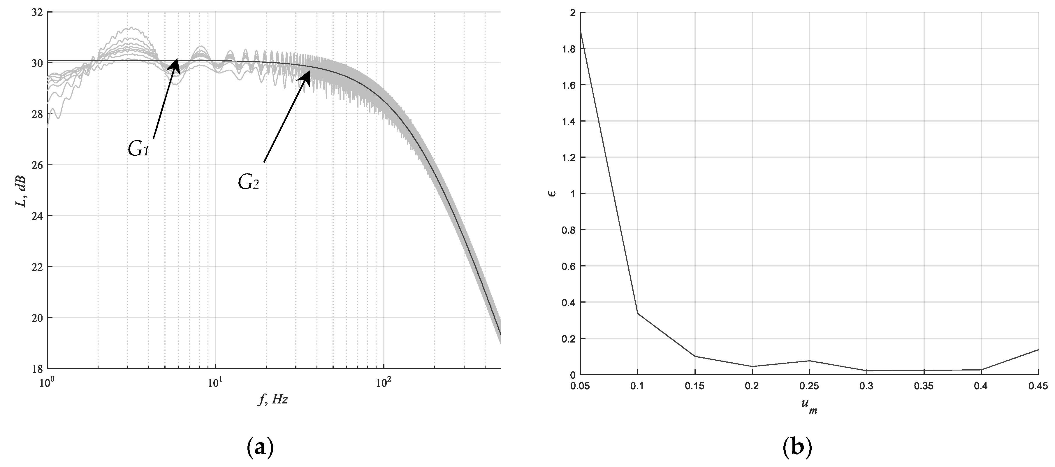
4.3. Data Processing

The estimation using the Fourier transform is asymptotically unbiased, and the frequency resolution increases with the increase in the number of samples N. However, the Fourier transform allows us to investigate the signal only in the frequency domain and does not contain any information about the time characteristics of the signal. The presence of noise or distortion in the experimental data leads to distortion of the estimation results: the estimation variance is determined by the signal-to-noise ratio and does not decrease with an increase in the number of samples or decreasing the sampling period. The described features make the empirical estimation of the FRF by Equation (15) rather inaccurate. This is explained by the fact that no specific features of experimental data are used in the estimation and there is no data compression [31,33,39].

One of the common approaches to reducing the variance of the estimated FRF is the splitting of the experimental data set from N samples into M segments by R samples. Then an empirical estimation is made for each segment:

$${\widehat{\widehat{G}}}_R^{(k)}\left(f\right)=\frac{{\displaystyle \sum _{n=0}^{R-1}{y}_n^{(k)}\exp (-j\cdot 2\pi \cdot f\cdot n\cdot T_d)}}{{\displaystyle \sum _{n=0}^{R-1}{u}_n^{(k)}\exp (-j\cdot 2\pi \cdot f\cdot n\cdot T_d)}}, k=1,2,\dots ,M$$

The final estimation is calculated as an arithmetic mean:

$${\widehat{G}}_N\left(f\right)=\frac{1}{M}{\displaystyle \sum _{k=1}^M{\widehat{\widehat{G}}}_{R k}^{(k)}\left(f\right)},$$

(18)

The disadvantage of the experimental data splitting is the appearance of the frequency spectrum distortions at the boundaries of the segments (leakage effect). To minimize this effect, the Fourier window transformation is used [33,39].

For each segment, the Fourier transform is made, and the result is multiplied by the weight function (window) [33,39], then the empirical estimation of the transfer function for the data segment is expressed as follows:

$${\widehat{\widehat{G}}}_{RW}^{(k)}\left(f\right)=\frac{{\displaystyle \sum _{n=0}^{R-1}{y}_n^{(k)}{w}_n^{(k)}\exp (-j\cdot 2\pi \cdot f\cdot n\cdot T_d)}}{{\displaystyle \sum _{n=0}^{R-1}{u}_n^{(k)}{w}_n^{(k)}\exp (-j\cdot 2\pi \cdot f\cdot n\cdot T_d)}}, k=1,2,\dots ,M$$

where w_n is values of the weight function.

The final estimation result is formed as an arithmetic mean similar to the expression in (18). This estimation technique is called the Bartlett’s periodogram method [39].

Then, overlapping of the data segments can be used to increase the number of considered data segments. It provides to reduce the variance of the FRF estimate. This technique is called the Welch’s method of modified periodograms.

In the described methods of experimental data processing, the input and output signals of the system are considered separately, and the FRF is defined as the ratio of the transformed signals. Separate processing of the system input and output signals may result in loss of information about the dynamic properties of controlled plant [33,34,35]. For the aggregate analysis of the input and output signals and the primary data filtration the Blackman–Tukey method [33] or the preliminary estimation of the impulse transient response [39] can be used.

According to the Blackman–Tukey method, the autocorrelation functions and the cross-correlation function for u_n and y_n signals are calculated at first:

$${\widehat{R}}_y\left(\tau \right)=\frac{1}{N}{\displaystyle \sum _{n=1}^N{y}_{n+\tau }{y}_n}, {\widehat{R}}_u\left(\tau \right)=\frac{1}{N}{\displaystyle \sum _{n=1}^N{u}_{n+\tau }{u}_n}, {\widehat{R}}_{yu}\left(\tau \right)=\frac{1}{N}{\displaystyle \sum _{n=1}^N{y}_{n+\tau }{u}_n}.$$

Then the short-time Fourier transform is calculated for these functions:

$$\begin{array}{l}{\widehat{\Phi }}_y\left(f\right)={\displaystyle \sum _{\tau =-M}^M{\widehat{R}}_y\left(\tau \right)w_M(\tau )\exp (-j\cdot 2\pi \cdot f\cdot \tau \cdot T_d)},\\ {\widehat{\Phi }}_u\left(f\right)={\displaystyle \sum _{\tau =-M}^M{\widehat{R}}_u\left(\tau \right)w_M(\tau )\exp (-j\cdot 2\pi \cdot f\cdot \tau \cdot T_d)},\\ {\widehat{\Phi }}_{yu}\left(f\right)={\displaystyle \sum _{\tau =-M}^M{\widehat{R}}_{yu}\left(\tau \right)w_M(\tau )\exp (-j\cdot 2\pi \cdot f\cdot \tau \cdot T_d)}.\end{array}$$

where w_M is values of the weight function.

The FRF estimation is expressed as follows:

$${\widehat{G}}_N\left(f\right)=\frac{{\widehat{\Phi }}_{yu}\left(f\right)}{{\widehat{\Phi }}_u\left(f\right)}.$$

The choice of window (weight) function in the short-time Fourier transform is carried out empirically, based on the ratio between the width of the main lobe and attenuation of the side lobes.

There are a lot of types of window functions, for example: rectangular window, Bartlett triangular window, Hann window, Hamming window, Blackman–Harris window, Kaiser–Bessel window, Dolph–Chebyshev window, and others. The last three windows are named as the preferred window functions for spectral analysis of signals [39].

The input and output signals of the dynamic system are related by the impulse transient response as follows:

$$y_n={\displaystyle \sum _{k=0}^{m-1}{g}_k{u}_{n-k}{T}_d+e_n}, n=m-1,\dots ,N-1$$

(19)

where g_k is an impulse transient response of the dynamic system, and e_n is a nonlinear component (noise).

Equation (19) can be written in the matrix form as follows:

$$\left[\begin{array}{c}{y}_{m-1}\\ y_m\\ y_{m+1}\\ ⋮\\ y_{N-1}\end{array}\right]=T_d\left[\begin{array}{cccc}{u}_{m-1}& u_{m-2}& \cdots & u_0\\ u_m& u_{m-1}& \cdots & u_1\\ u_{m+1}& u_m& \cdots & u_2\\ ⋮& ⋮& \ddots & ⋮\\ u_{N-1}& u_{N-2}& \cdots & u_{N-m}\end{array}\right]\left[\begin{array}{c}{g}_0\\ g_1\\ ⋮\\ g_{m-1}\end{array}\right]+\left[\begin{array}{c}{e}_{m-1}\\ e_m\\ e_{m+1}\\ ⋮\\ e_{N-1}\end{array}\right],$$

or

$$y=Ug+e.$$

The estimation of the impulse transient response ĝ can be found using the least squares method by taking the pseudo-inverse matrix, which is given by the following equation [33]:

$$\widehat{g}={(U^{T}U)}^{-1}(U^{T}y),$$

The FRF estimation in this case can be obtained using the Fourier transform:

$$\widehat{G}\left(f_n\right)={\displaystyle \sum _{n=0}^{N-1}{\widehat{g}}_n\exp (-j\cdot 2\pi \cdot f\cdot n\cdot T_d)}$$

The estimation of the impulse transient response provides the compression of the considered data set to m samples, thus providing some noise filtration.

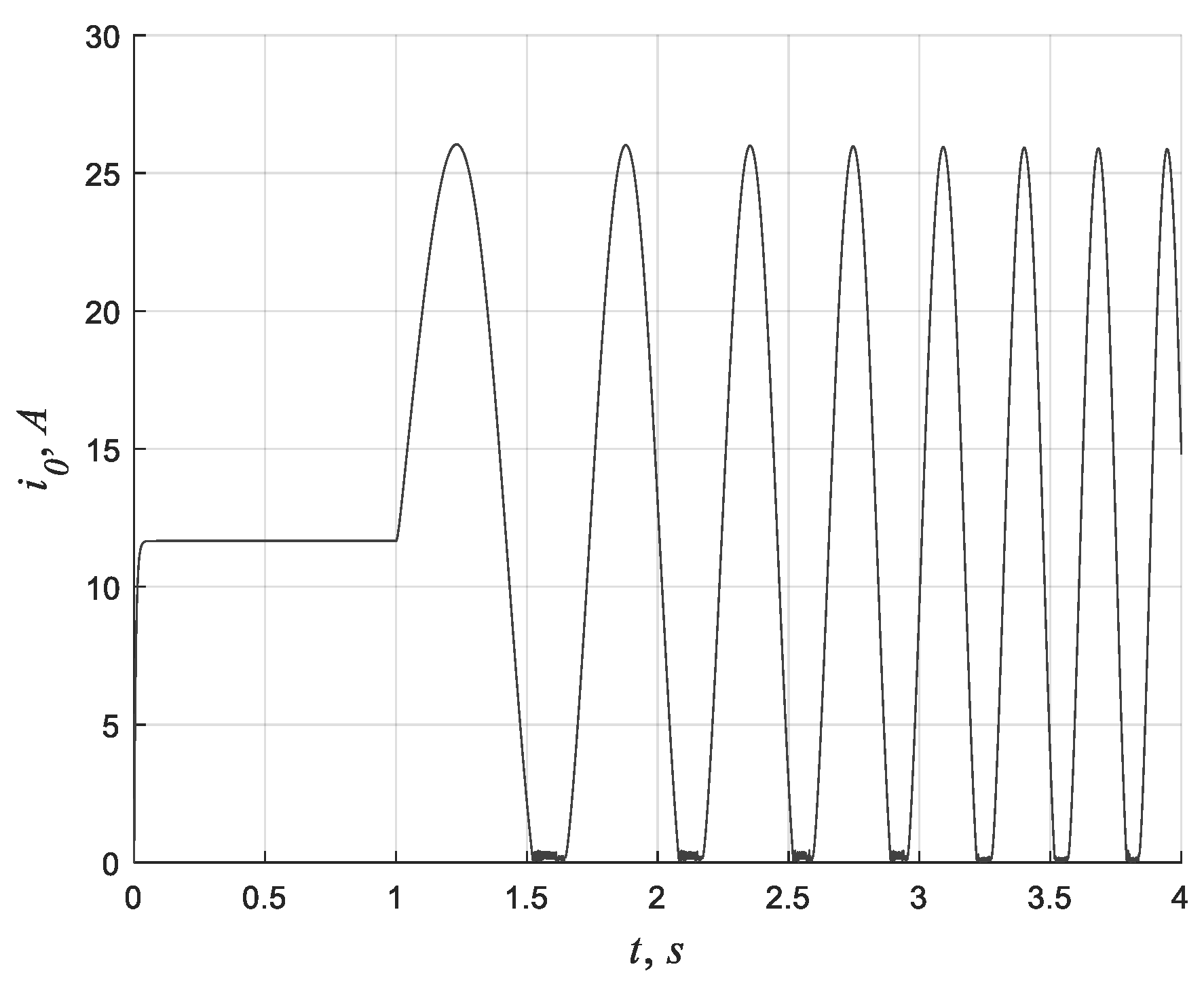
4.4. Simulation Results

Figure 9 shows the results of the FRF estimation by the Blackman–Tukey method. Figure 10 shows the results of the FRF estimation by the impulse transient response estimation method. The proposed techniques of data processing allow us to minimize the variance of the FRF estimation in the presence of measurement noise.

Figure 11 shows the results of the K_inv and T_e estimation by the FRFs estimated by the method based on the estimation of the impulse transient response which are presented in Figure 10. Presented results of K_inv and T_e estimation correspond to their real values with high accuracy.

Figure 10 and Figure 11 show that the inaccuracy of FRF and SPMSM parameter estimation increases at the amplitudes of the chirp signal which are equal to 0.05 and 0.45. If the amplitude of the chirp-signal is equal to 0.45 and the constant component is equal to 0.5, the lower bound of the excitation signal gets into the «dead zone» of the PWM inverter. This effect has been described after Figure 5. The reasons for the decrease of the estimation accuracy at the amplitude of the chirp-signal equal to 0.05 are quite obvious. If the amplitude of the chirp-signal is small negative influence of measurement noise on estimation results increases.

5. Discussion

It is shown in the paper that the dead time effect in PWM inverters has a negative impact on the results of parameter identification of the SPMSM. A modified technique of parameter identification of the SPMSM based on the estimation of the FRF is proposed. It allows to estimate the parameters of the linear transfer function of the SPMSM in the presence of the dead time effect and measurement noise with the sufficient accuracy for tuning the current (torque) control loop.

The proposed design of identification experiment provides the absence of the SPMSM torque by software methods. It allows us to avoid uncontrolled rotation of the electric drive during the experiment. An excitation input signal is formed from a constant component and sinusoidal signal with linear frequency modulation (chirp signal). The presence of a constant component allows us to minimize the influence of dead time effect of the PWM inverter on the results of the experiment. It is shown that estimation of SPMSM parameters by experimental FRF allows us to get better results than by time series of data in this case. In the absence of measurements noise, empirical estimation of the FRF is a sufficient method for parameter estimation and experimental data analysis. In the presence of the measurements noise, the minimum variance of the FRF estimation is provided by the data processing method based on the estimation of the impulse transient response. The amplitude of the chirp-signal and the value of the constant component should be selected so that the lower bound of the signal is more than 2τ and the upper bound of the signal does not exceed the SPMSM current limit. The minimal amplitude of the chirp-signal, which is sufficient for identification, should be selected based on the level of the measurement noise.

The applicability of estimation for the electrical time constant of SPMSM using this technique is limited by the half of the sampling frequency of the current (torque) control loop (Nyquist frequency) and by the zero-order hold effect on high frequencies.

References

1. Krause, P.C.; Wasynczuk, O.; Sudhoff, S.D. Analysis of Electric Machinery; McGraw-Hill: New York, NY, USA, 1986; Volume 564. [Google Scholar]
2. Bose, B.K. Modern Power Electronics and AC Drives; Prentice Hall: Upper Saddle River, NJ, USA, 2002; Volume 123. [Google Scholar]
3. Pillay, P.; Krishnan, R. Modeling, simulation, and analysis of permanent-magnet motor drives. I. The permanent-magnet synchronous motor drive. IEEE Trans. Ind. Appl. 1989, 25, 265–273. [Google Scholar] [CrossRef]
4. Lovlin, S.; Abdullin, A. Adaptive system for compensation of periodic disturbances in servo drive. In Proceedings of the 2016 IX International Conference on Power Drives Systems (ICPDS), Perm, Russia, 3–7 October 2016; pp. 1–5. [Google Scholar]
5. Holtz, J.; Springob, L. Identification and compensation of torque ripple in high-precision permanent magnet motor drives. IEEE Trans. Ind. Electron. 1996, 43, 309–320. [Google Scholar] [CrossRef] [Green Version]
6. Mora, A.; Orellana, Á.; Juliet, J.; Cardenas, R. Model Predictive Torque Control for Torque Ripple Compensation in Variable Speed PMSMs. IEEE Trans. Ind. Electron. 2016, 63, 4584–4592. [Google Scholar] [CrossRef]
7. Shao, M.; Deng, Y.; Li, H.; Liu, J.; Fei, Q. Sliding Mode Observer-Based Parameter Identification and Disturbance Compensation for Optimizing the Mode Predictive Control of PMSM. Energies 2019, 12, 1857. [Google Scholar] [CrossRef]
8. Ding, X.; Wang, S.; Zou, M.; Liu, M. Predictive Current Control for Permanent Magnet Synchronous Motor Based on MRAS Parameter Identification. In Proceedings of the IEEE International Power Electronics and Application Conference and Exposition (PEAC), Shenzhen, China, 4–7 November 2018; pp. 1–5. [Google Scholar]
9. Urbanski, K.; Janiszewski, D. Sensorless Control of the Permanent Magnet Synchronous Motor. Sensors 2019, 19, 3546. [Google Scholar] [CrossRef] [PubMed]
10. Ortega, R.; Monshizadeh, N.; Monshizadeh, P.; Bazylev, D.; Pyrkin, A. Permanent magnet synchronous motors are globally asymptotically stabilizable with PI current control. Automatica 2018, 98, 296–301. [Google Scholar] [CrossRef] [Green Version]
11. Beltran-Carbajal, F.; Tapia-Olvera, R.; Lopez-Garcia, I.; Valderrabano-Gonzalez, A.; Rosas-Caro, J.C.; Hernandez-Avila, J.L. Extended PI Feedback Tracking Control for Synchronous Motors. Int. J. Control Autom. Syst. 2019, 17, 1346–1358. [Google Scholar] [CrossRef]
12. Qiao, W.; Tang, X.; Zheng, S.; Xie, Y.; Song, B. Adaptive two-degree-of-freedom PI for speed control of permanent magnet synchronous motor based on fractional order GPC. ISA Trans. 2016, 64, 303–313. [Google Scholar] [CrossRef] [PubMed]
13. Orłowska-Kowalska, T.; Lovlin, S.Y.; Tsvetkova, M.H.; Abdullin, A.A.; Mamatov, A.G. Parametric identification of a servo drive model with deadtime-type nonlinearities. J. Instrum. Eng. 2019, 62, 576–584. [Google Scholar]
14. Urasaki, N.; Senjyu, T.; Uezato, K.; Funabashi, T. Adaptive Dead-Time Compensation Strategy for Permanent Magnet Synchronous Motor Drive. IEEE Trans. Energy Convers. 2007, 22, 271–280. [Google Scholar] [CrossRef]
15. Anuchin, A.; Gulyaeva, M.; Briz, F.; Gulyaev, I. Modeling of AC voltage source inverter with dead-time and voltage drop compensation for DPWM with switching losses minimization. In Proceedings of the International Conference on Modern Power Systems (MPS), Cluj-Napoca, Romania, 6–9 June 2017; pp. 1–6. [Google Scholar]
16. Zhang, H.; Kou, B.; Zhang, L.; Zhang, H. Analysis and Compensation of Dead-Time Effect of a ZVT PWM Inverter Considering the Rise- and Fall-Times. Appl. Sci. 2016, 6, 344. [Google Scholar] [CrossRef]
17. Ji, Y.; Yang, Y.; Zhou, J.; Ding, H.; Guo, X.; Padmanaban, S. Control Strategies of Mitigating Dead-time Effect on Power Converters: An Overview. Electronics 2019, 8, 196. [Google Scholar] [CrossRef]
18. Qiu, T.; Wen, X.; Zhao, F. Adaptive-Linear-Neuron-Based Dead-Time Effects Compensation Scheme for PMSM Drives. IEEE Trans. Power Electron. 2016, 31, 2530–2538. [Google Scholar] [CrossRef]
19. Diallo, D.; Arias, A.; Cathelin, J. An inverter dead-time feedforward compensation scheme for PMSM sensorless drive operation. In Proceedings of the 2014 First International Conference on Green Energy (ICGE), Sfax, Tunisia, 25–27 March 2014; pp. 296–301. [Google Scholar]
20. Munoz, A.R.; Lipo, T.A. On-line dead-time compensation technique for open-loop PWM-VSI drives. IEEE Trans. Power Electron. 1999, 14, 683–689. [Google Scholar] [CrossRef]
21. Haifeng, X.; Yuyao, H. Compensation of dead-time effects based on adaptive voltage disturbance estimator in PMSM drives. In Proceedings of the 26th Chinese Control and Decision Conference (CCDC), Changsha, China, 31 May–2 June 2014; pp. 3439–3444. [Google Scholar]
22. Chen, Y.; Zhou, F.; Liu, X. Online adaptive parameter identification of PMSM based on the dead-time compensation. Int. J. Electron. 2014, 102, 1132–1150. [Google Scholar] [CrossRef]
23. Jonsky, T.; Stichweh, H.; Theßeling, M.; Wettlaufer, J.; Quattrone, F. Modeling and parameter identification of multiphase permanent magnet synchronous motors including saturation effects. In Proceedings of the 17th European Conference on Power Electronics and Applications (EPE’15 ECCE-Europe), Geneva, Switzerland, 8–10 September 2015; pp. 1–10. [Google Scholar]
24. Ding, F.; Pan, J.; Alsaedi, A.; Hayat, T. Gradient-Based Iterative Parameter Estimation Algorithms for Dynamical Systems from Observation Data. Mathematics 2019, 7, 428. [Google Scholar] [CrossRef]
25. Liling, S.; Heming, L.; Boqiang, X. Precise determination of permanent magnet synchronous motor parameters based on parameter identification technique. In Proceedings of the Sixth International Conference on Electrical Machines and Systems (ICEMS), Beijing, China, 9–11 November 2003; Volume 1, pp. 34–36. [Google Scholar]
26. Lu, H.; Wang, Y.; Yuan, Y.; Zheng, J.; Hu, J.; Qin, X. Online identification for permanent magnet synchronous motor based on recursive fixed memory least square method under steady state. In Proceedings of the 36th Chinese Control Conference (CCC), Dalian, China, 26–28 July 2017; pp. 4824–4829. [Google Scholar]
27. Vaseghi, B.; Takorabet, N.; Meibody-Tabar, F. Fault Analysis and Parameter Identification of Permanent-Magnet Motors by the Finite-Element Method. IEEE Trans. Magn. 2009, 45, 3290–3295. [Google Scholar] [CrossRef]
28. Pulvirenti, M.; Scarcella, G.; Scelba, G.; Testa, A.; Harbaugh, M.M. On-Line Stator Resistance and Permanent Magnet Flux Linkage Identification on Open-End Winding PMSM Drives. IEEE Trans. Ind. Appl. 2019, 55, 504–515. [Google Scholar] [CrossRef]
29. Folgheraiter, M. A combined B-spline-neural-network and ARX model for online identification of nonlinear dynamic actuation systems. Neurocomputing 2016, 175, 433–442. [Google Scholar] [CrossRef]
30. Schoukens, J.; Pintelon, R.; Dobrowiecki, T.; Rolain, Y. Identification of linear systems with nonlinear distortions. Automatica 2005, 41, 491–504. [Google Scholar] [CrossRef]
31. Ljung, L. System Identification. In Encyclopedia of Electrical and Electronics Engineering; American Cancer Society, Wiley: New York, NY, USA, 1999; ISBN 978-0-471-34608-1. [Google Scholar]
32. Hägg, P.; Hjalmarsson, H.; Wahlberg, B. A least squares approach to direct frequency response estimation. In Proceedings of the 50th IEEE Conference on Decision and Control and European Control Conference, Orlando, FL, USA, 12–15 December 2011; pp. 2160–2165. [Google Scholar]
33. Ilvedson, C.R. Transfer Function Estimation Using Time-Frequency Analysis. Ph.D. Thesis, Massachusetts Institute of Technology, Cambridge, MA, USA, 1998. [Google Scholar]
34. Samygina, E.; Tiapkin, M.; Rassudov, L.; Balkovoi, A. Extended Algorithm of Electrical Parameters Identification via Frequency Response Analysis. In Proceedings of the 26th International Workshop on Electric Drives: Improvement in Efficiency of Electric Drives (IWED), Moscow, Russia, 30 January–2 February 2019; pp. 1–4. [Google Scholar]
35. Feron, E.; Brenner, M.; Paduano, J.; Turevskiy, A. Time-Frequency Analysis for Transfer Function Estimation and Application to Flutter Clearance. J. Guid. Control Dyn. 1998, 21, 375–382. [Google Scholar] [CrossRef]
36. Saupe, F.; Knoblach, A. Experimental determination of frequency response function estimates for flexible joint industrial manipulators with serial kinematics. Mech. Syst. Signal Process. 2015, 52, 60–72. [Google Scholar] [CrossRef]
37. Ljung, L.; Glover, K. Frequency domain versus time domain methods in system identification. Automatica 1981, 17, 71–86. [Google Scholar] [CrossRef]
38. Villwock, S.; Pacas, M. Application of the Welch-Method for the Identification of Two- and Three-Mass-Systems. IEEE Trans. Ind. Electron. 2008, 55, 457–466. [Google Scholar] [CrossRef]
39. Ifeachor, E.C.; Jervis, B.W. Digital Signal Processing: A Practical Approach; Pearson Education: London, UK, 2002; ISBN 978-0-201-59619-9. [Google Scholar]
40. Nussbaumer, T.; Heldwein, M.L.; Gong, G.; Round, S.D.; Kolar, J.W. Comparison of Prediction Techniques to Compensate Time Delays Caused by Digital Control of a Three-Phase Buck-Type PWM Rectifier System. IEEE Trans. Ind. Electron. 2008, 55, 791–799. [Google Scholar] [CrossRef]
41. Ma, J.; Wang, X.; Blaabjerg, F.; Harnefors, L.; Song, W. Accuracy Analysis of the Zero-Order Hold Model for Digital Pulse Width Modulation. IEEE Trans. Power Electron. 2018, 33, 10826–10834. [Google Scholar] [CrossRef] [Green Version]
42. Mizutani, R.; Takeshita, T.; Matsui, N. Current model-based sensorless drives of salient-pole PMSM at low speed and standstill. IEEE Trans. Ind. Appl. 1998, 34, 841–846. [Google Scholar] [CrossRef]
43. Wang, G.; Kuang, J.; Zhao, N.; Zhang, G.; Xu, D. Rotor Position Estimation of PMSM in Low-Speed Region and Standstill Using Zero-Voltage Vector Injection. IEEE Trans. Power Electron. 2018, 33, 7948–7958. [Google Scholar] [CrossRef]
Figure 1. The direction of the current during the dead-time in one phase of the three-phase pulse width modulated (PWM) inverter.
Electronics 08 01200 g001
Figure 2. Phase current distortion and surface mounted permanent magnet synchronous motor (SPMSM) torque distortion caused by the dead-time of the PWM inverter: (a) the current in one phase of the SPMSM with an ideal PWM inverter (IA) and the current in corresponding phase of the SPMSM in presence of dead-time (IA_dt), (b) the SMPM torque in the system with an ideal PWM inverter (M) and in a system with an PWM inverter with dead-time (Mdt).
Electronics 08 01200 g002
Figure 3. Results of Kinv and Te estimation without taking into account the dead time effect: (a) Kinv_1 is a real value of the parameter, Kinv_2 is the value estimated by the data in time domain, Kinv_3 is the value estimated by the data in frequency domain, (b) Te_1 is a real value of the parameter, Te_2 is the value estimated by the data in time domain, Te_3 is the value estimated by the data in frequency domain.
Electronics 08 01200 g003
Figure 4. The step response of the closed current (torque) loop with the linear digital proportional-integral controller, TT = 3 μs: 1—proportional-integral controller is tuned with nominal SPMSM parameters, 2—proportional-integral controller is tuned with SPMSM parameters estimated without considering the dead time effect (amplitude of the meander of the generalized voltage u0 is 0.6).
Electronics 08 01200 g004
Figure 5. Results of Kinv and Te estimation with modified excitation input signal: (a) Kinv_1 is a real value of the parameter, Kinv_2 is the value estimated by the data in the time domain, Kinv_3 is the value estimated by the data in the frequency domain, (b) Te_1 is a real value of the parameter, Te_2 is the value estimated by the data in the time domain, Te_3 is the value estimated by the data in the frequency domain.
Electronics 08 01200 g005
Figure 6. Results of the frequency response function (FRF) estimation by the empirical method in absence of measurement noise: (a) G1 is the reference FRF, G2 is the estimated FRFs (b) standard error of estimation.
Electronics 08 01200 g006
Figure 7. Shape of the generalized current i0 at identification experiment with the amplitude of the chirp-signal equal to 0.45.
Electronics 08 01200 g007
Figure 8. Results of the FRF estimation by empirical method in presence of measurement noise: (a) G1 is the reference FRF, G2 is the estimated FRFs, (b) standard error of estimation.
Electronics 08 01200 g008
Figure 9. Results of the FRF estimation by the Blackman–Tukey method in presence of measurement noise: (a) G1 is the reference FRF, G2 is the estimated FRFs, (b) standard error of estimation.
Electronics 08 01200 g009
Figure 10. Results of the FRF estimation by the method based on the estimation of the impulse transient response in presence of measurement noise: (a) G1 is the reference FRF, G2 is the estimated FRFs, (b) standard error of estimation.
Electronics 08 01200 g010
Figure 11. Results of Kinv and Te estimation with modified excitation input signal: (a) Kinv_1 is a real value of the parameter, Kinv_2 is the value estimated by the data in time domain, Kinv_3 is the value estimated by the data in frequency domain, (b) Te_1 is a real value of the parameter, Te_2 is the value estimated by the data in time domain, Te_3 is the value estimated by the data in frequency domain.
Electronics 08 01200 g011