Abstract
Land environment is one of the most commonly and importantly used synthetical natural environments in a virtual test. To recognize the ground truth for the construction of virtual land environment, a deep transfer hyperspectral image (HSI) classification method based on information measure and optimal neighborhood noise reduction was proposed in this article. Firstly, the information measure method was used to select the most valuable spectrum. Specifically, three representative bands were selected using the combination of entropy, color matching function, and mutual information. Based on the selected bands, a patch containing spatial-spectral information was constructed and used as the input of the convolutional neural networks (CNN) network. Then, in order to address the problem that a large number of labeled samples were required in deep learning method, the HSI classification method based on deep transfer learning was proposed. In the proposed method, the transfer of parameters ensured the classification performance with small training samples and reduced the training cost. Moreover, the optimal neighborhood noise reduction was used as the post-processing method to effectively eliminate the salt-and-pepper noise and further improve the classification performance. Experiments on two datasets demonstrated that the proposed method in this article had higher classification accuracy than similar methods.
1. Introduction
In recent years, hyperspectral image (HSI) analysis has been widely used in various fields [1], such as the monitoring of land cover change [2,3] and the environmental science and mineral development [4]. As an advanced machine learning technology, deep learning has been widely used in image classification to learn the hierarchical features of a deep neural network from low-level to high-level [5]. The image classification methods based on the convolutional neural networks (CNN) have shown the ability to detect local features of the hyperspectral input data and obtain the classification results with high accuracy and stability. Rachmadi et al. proposed an adaptation of a convolutional neural network (CNN) scheme proposed for segmenting brain lesions with considerable mass-effect, to segment white matter hyperintensities (WMH) characteristic of brains with none or mild vascular pathology in routine clinical brain magnetic resonance images (MRI) [6]. Krizhevsky et al. proposed a large, deep convolutional neural network to classify the 1.2 million-high resolution images in the ImageNet LSVRC-2010 contest into the 1000 different classes [7]. In addition to the application in common image classification, many CNN-based hyperspectral image classification methods have been developed in recent years. Ma et al. proposed a context deep-learning algorithm for learning the features, which can better characterize the information than the extraction algorithms with predefined features [8]. Zhang et al. proposed a region-based diversified CNN, which can semantically encode context-aware representations to obtain valuable features and improve the classification accuracy [9]. Chen et al. first proposed the Stack Automated Encoder (SAE) framework to incorporate the features with the special-spectral information. Firstly, the validity of SAE was verified by the classical spectral information-based classification method. Secondly, a new classification method based on spatial principal component information was proposed [10]. Slavkovikj et al. proposed a CNN framework for hyperspectral image classification in which spectral features were extracted from a small neighborhood [11]. Makantasis et al. proposed an R-PCA CNN classification method [12], in which PCA was first used to extract the spatial information, and then CNN was used to encode spectral and spatial information. The CNN classification methods with the combined spectral and spatial information have shown better classification performance.
The hyperspectral image contains all of the spectral information of the ground objects, with the typical high-dimensional features. However, the spectral information with high redundancy may interfere with the classification process and reduce the classification accuracy. Therefore, it is very important to reduce the spectral dimensionality of the hyperspectral image before the classification process. Two typical dimensionality-reduction methods have been reported, i.e., feature extraction and band selection methods. The feature extraction method mainly included principal component analysis (PCA) [13], linear discriminant analysis (LDA) [14], and multidimensional scaling [15]. The band selection method mainly included examining correlations [16], calculating mutual information [17,18], etc.. In recent years, information-based band selection has been a very popular research topic, in which the Shannon entropy or its changes, such as mutual information (MI), were usually used as the basis of image information measure. Bajcsy proposed a band selection method under the constraints of classification accuracy and computational requirements, in which the optimal number of bands was determined by the unsupervised method of entropy [19]. Adolfo proposed a clustering method for automatic band selection based on the mutual information in multispectral images [20]. Wang proposed a supervised classification method for band selection based on spatial entropy [21]. Le Moan et al. proposed a new spectral image visualization method to achieve band selection by the first-order, second-order, and third-order information measure [22]. Manel proposed a frequency band selection method based on the hierarchical clustering of spectral layer, and used mutual information measure to reduce the dimensions of the image. Then a new c-means clustering algorithm was proposed to integrate the spatial spectrum information [23]. Hossain et al. proposed a dimensionality reduction method (PCA-nMI) that combined principal component analysis (PCA) with normalized mutual information (nMI) under two constraints [24]. The proposed method maximized the general correlation and minimized the redundancy in selected subspaces.
In the application of the deep neural networks to the classification of hyperspectral images, there were some difficulties in the process of model training, such as the high demand for training samples and the time complexity of computing models. Transfer learning can address the above difficulties to some extent. In transfer learning, the learned knowledge or experience from the source tasks is applied to the object tasks. Based on transfer learning, Li et al. proposed a CNN framework for the anomaly detection [25] and the training of multi-layer CNNs using the differences between adjacent pixels generated from the source image dataset. The experimental performance showed that the proposed algorithm was superior to the classical Reed-Xiaoli [26] and the most advanced representation-based detectors, such as sparse representation-based detectors (SRD) [27] and cooperative representation-based detectors [28]. Wang proposed two architectures to extract the general features of remote scene classification from the pre-trained CNNs [29]. Wang Liwei et al. proposed a hyperspectral image classification method by applying transfer learning in deep residual networks [30], and shared the shallow network weight parameters of deep residual networks. At the same time, in order to address the over-fitting problem in the process of transfer shallow network parameters from the large source dataset to the small object dataset, the strategy of fine-tuning the residual network was proposed, in which the deep layer of deep residual network was randomly initialized and retrained in the object dataset.
The method studied in this article is to construct a virtual land environment for virtual test, which is also one of the research fields of the author’s team. In order to build a virtual land environment which can be used as the basis of other natural environment modeling and sensor sensing, the most important thing is to accurately acquire the information of ground truth. So, we propose a scheme to construct the virtual land environment using multi-source satellite’s earth observation data. The method proposed in this paper is the key step of ground truth recognition. In this article, the hyperspectral image classification method based on CNN was investigated. In addition, the information measure was used to select the bands and reduce the dimensionality of hyperspectral images, thus, reducing the redundant information. At the same time, the spatial-spectral features were extracted to improve the classification performance of hyperspectral images. Furthermore, the classification method based on deep transfer learning and neighborhood noise reduction was used to achieve high classification accuracy for small-sized samples and reduce the training complexity of the object dataset.
2. The Related Work
The method studied in this article is to build a virtual land environment, which belongs to the field of virtual tests. Virtual test technology is a new test technology. Because of its low cost, high efficiency and ability to support test in a complex environment, virtual test technology has been more and more widely used, such as automobile test [31], building design [32], weapon system test [33] and so on. The virtual test is inseparable from the virtual environment, so in order to meet the needs of the virtual test in a complex environment, it is an important research content to study the modeling theory and method of all kinds of complex environments. The synthetic natural environment, which is composed of land, atmosphere, ocean and space environment, is the space for various human activities [34]. The virtual land environment is one of the important components of the virtual natural environment. The current virtual land environment, which is often used in virtual reality [35] and visual simulation [36], is mainly concerned about visualization and pays attention to the immersion. However, the new virtual test puts higher demands on the virtual land environment, as follows.
(1) Providing support for the construction of other types of natural environment. The synthetic natural environment is an interrelated and interactive organic whole, especially the interaction between the land environment and the atmospheric environment. For example, the MM5 atmospheric model needs six types of land environmental data, such as land surface type, water body, vegetation composition, etc. [37].
(2) Providing a sensing basis for virtual sensors. For example, when using infrared imaging sensors to detect the ground, it is necessary to support the high-precision three-dimensional land environment with the information of ground truth, material, etc.
Based on the above analysis, the virtual land environment used in the virtual test is more important to be used as the modeling basis of other natural environments and the sensing basis of various sensors. What is more, it is a three-dimensional land environment which contains various information, such as ground truth, objects material, color, texture, etc. Therefore, as shown in Figure 1, we propose a scheme to construct a virtual land environment using multi-source satellite earth observation data, which is a joint application of multi-sensor data [38]. Based on hyperspectral, multispectral, panchromatic, and other optical earth observation data and radar earth observation data, such as InSAR, the construction of virtual land environment is completed through four steps: Temporal-spatial-spectral fusion (A), ground truth recognition (B), elevation extraction (C) and synthesis (D). Among them, ground truth recognition (B) is a key step, which is responsible for providing accurate information, such as ground truth, material, etc for the virtual land environment. The HSI classification method proposed in this article belongs to this step, and the ground truth information is obtained through the classification of HSI.
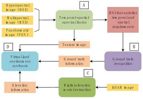
Figure 1.
The process of constructing a virtual land environment using multi-source satellite Earth observation data.
In the virtual test, according to the test requirements, a specific space range of virtual land environment is usually constructed, which may use the earth observation data obtained by different sensors. At the same time, the method of ground truth classification based on machine learning needs a large number of marked data as training samples. It is not easy to prepare a large amount of marked data for the images of different scenes obtained by different sensors. Therefore, transfer learning is adopted in this article. After training the classification network in all kinds of typical scenes, we can transfer to a specific scene and do a little training.
3. Dimensionality Reduction of Hyperspectral Image Based on Information Measure
3.1. Spectral Band Preprocessing Based on Entropy and Color Matching Function (CMF)
Based on the information theory, Shannon first proposed the concept of entropy in 1948 [39], in which the amount of information with uncertainty, i.e., the probability of the occurrence of discrete random events was measured. The greater amount of information indicated a smaller redundancy. The information measure based on Shannon’s communication theory has been proven very effective in identifying the redundancy of high-dimensional datasets.
The entropy of a random variable is defined as
where is the event of , is the probability density function of , and b is the logarithmic order.
Assume and are two random variables, where has n values and has m values. Then their joint entropy is
where is the joint probability density function of and .
When these measurements are applied to hyperspectral images, it is generally assumed that each channel (spectral band) is equivalent to a random variable , and each pixel in the channel is an event . In the preprocessing step for the spectral band of the hyperspectral image, the channel with less information is eliminated based on Shannon entropy, which are described as follows:
Firstly, the entropy of each spectral band of the hyperspectral image is calculated. The random variable is the i-th spectral band (i = 1, 2, ... n), is the pixel of the i-th spectral band, and is the probability density function of the band .
Secondly, the local average entropy of each spectral band is defined as Equation (4), where m is the window size, indicating the size of the neighborhood.
Finally, the bands that meet the following conditions are retained.
where is the threshold factor. The spectral band with higher or lower entropy than the range of of the local average entropy is considered to be irrelevant.
The blue line in Figure 2 is the entropy curve, in which the horizontal axis represents the spectral dimension and the vertical axis represents the entropy of each spectral band. The smoothness of the entropy curve determines the window size m and the threshold factor . If the entropy curve is smooth, the change of the adjacent spectral band information, i.e., the uncertainty of the band information is small; thus, the number of bands outside the relevant range, i.e., the probability of having an uncorrelated band, is also small. In this condition, few spectral bands are redundant, thus, smaller and m values should be chosen to improve the ability of excluding redundant bands. On the contrary, if the entropy curve fluctuates greatly, the change of the adjacent spectral band information, i.e., the uncertainty of the band information, is large; thus, the number of bands outside the correlation range, i.e., the probability of having an uncorrelated band, is also large. In this case, more spectral bands are redundant, thus, larger and m values should be chosen to exclude the redundant bands and retain the bands with valid information.
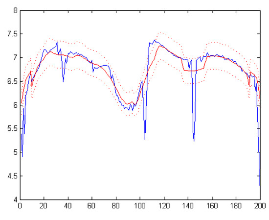
Figure 2.
Exclusion of the unrelated spectral bands of the Indian pines dataset.
The color matching function (CMF) in CIE 1931 standard chromaticity observer [40] described the human eye visual color characteristics. This function was used to achieve the complete process of preliminary selection of spectral bands based on the calculation of entropy. At a specific wavelength, the CMF determined the number of the three primary lights (red, blue and green), which must be mixed in a certain order to achieve the same visual effect as the corresponding monochrome light at that wavelength. By applying the CIE color matching to hyperspectral images in the visible range, hyperspectral images can be represented by the corresponding color matching [41].
As shown in Figure 3, the wavelength of the first effective spectral band was λ = 360 nm, and the wavelength of the last effective spectral band was nm. Then a linear interpolation was performed between the first and last effective spectral band.
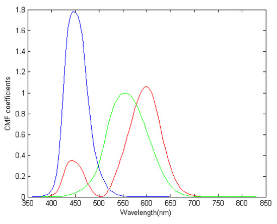
Figure 3.
CIE 1931 color matching curve between 360 nm and 830 nm.
In order to obtain the band selection sets, the thresholds t for the CMF coefficients of the three primary colors were set, i.e., , and were set based on the optical channels of the three primary colors.
In Figure 4, two spectral thresholds (t = 0.1, t = 0.5) were set for the coefficient variation curve of the CMF of the red light. When the CMF coefficient is above the threshold, the corresponding spectral bands were preserved. It was challenging to set the value of the parameter t without a specific application. In this article, an automatic threshold method was used to define the optimal threshold t to maximize the amount of discarded information. Use to label the set of channels which are discarded by threshold processing of the CMF and to label the complementary set of . The optimal threshold is defined as
where is the total entropy of the discarded spectral bands obtained by the above derivation, and is the total entropy of the selected spectral bands. Using the above describe method, the initially selected spectral bands can be obtained.
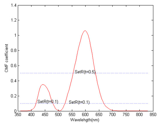
Figure 4.
Color matching function (CMF) coefficient changes of red light.
3.2. Band Selection Based on Mutual Information
Mutual Information (MI) is a measure of the useful information, which is defined as the amount of the information contained in a random variable about another random variable. The MI between two random variables X and Y is defined as
where is the probability density function of X, is the probability density function of Y, and is the joint probability density function of X and Y. H(X) is the entropy of the random variable X, and is the entropy of the random variable Y, which is calculated by Equation (1). is the joint entropy of two random variables X and Y, which can be calculated by Equation (2).
Furthermore, Bell proposed the mutual information of three random variables X, Y and Z, as shown in the following [42]:
where is the third-order joint entropy of three random variables X, Y and Z.
The above principle is equally applicable in hyperspectral images. The information of one channel can increase the mutual information between the other two channels. In this case, as the overlapped information between the two channels is less, the interdependence degree between the two random variables is lower, and the amount of contained information is greater. In the dimensionality reduction of hyperspectral images, it is necessary to consider both criteria, i.e., the largest amount of information and the least amount of redundancy.
Pla proposed the application of standardized mutual information [43]. In this article, we used the k-th order normalized information (NI) of the band as the standardized mutual information, in which NI is defined as
where is the mutual information of the bands to , and is the entropy of the band .
Three parts, , and , were obtained by setting threshold t for the CMF coefficients of the three primary colors. As the value of the mutual information was smaller, the amount of contained information in the selected spectral bands was larger, and the dimensionality reduction effect on the hyperspectral image was better. The spectral bands, , were obtained to minimize and selected as the most valuable bands.
3.3. Two Strategies for CNN Inputs
Three spectral bands, , were selected for the dimensionality reduction of hyperspectral image based on the information measure, and three grayscale images were obtained. There were two strategies to enter the CNN network, as shown in Figure 5. In the first strategy, the three spectral bands were directly used to extract the neighborhood around the pixel and classify the pixel into a patch of m × m × 3, which was put into the CNN for classification. This method was also called the information measure classification method (IM for short) because it directly used the dimensionality reduction results based on the information measure. In the second strategy, all the spectral information of the pixel was superimposed and classified on the above patch to form a patch of . All the spectral information of the central pixel of the patch was extracted, combined, intercepted, and reshaped. Then three layers of spectral information were obtained, which had the same shape and size as the three-dimensional spatial-spectral information extracted by the IM method. Then, the patch generated by the IM method and the new patch were superimposed and put into CNN for classification. In this article, the proposed method was called the information measure-spectral (IM-SPE for short) classification method.
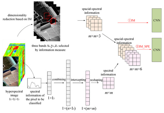
Figure 5.
The principle of dimensionality reduction based on the integration of information measure and spectral information.
The spectral information was processed as follows: Assume that the size of hyperspectral data was . At first, the one-dimensional spectral information of the central pixel with the size of was superimposed by n times to obtain the one-dimensional spectral information of . Then a one-dimensional spectral vector equal to was intercepted and reshaped to a two-dimensional spectral matrix of m × m. Then a spatial-spectral patch was obtained by superimposing three spectral information layers and combining the superimposed information with the three spatial-spectral information extracted by the IM method.
4. Hyperspectral Image Classification Method Based on Deep Transfer Learning
The classification of hyperspectral image based on deep transfer learning can be used to better solve the problem that the sample data is insufficient or relatively small. The specific classification principle is shown in Figure 6.
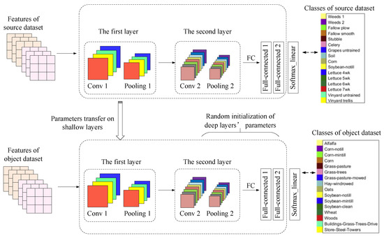
Figure 6.
Principle of hyperspectral image classification based on deep transfer learning.
Training was performed on the source dataset to obtain the network model and parameters. The shallow layer structure and parameters were directly transferred to the object dataset, and the deep layer parameters were randomly initialized. Taking the CNN network structure of Figure 6 as an example (including two convolutions and pooling layers, and two fully connected layers), if the source hyperspectral dataset is highly similar to the object hyperspectral dataset, the adjustment of the deep parameters should be in the following order: The last fully connected layer (full-connected2), the first fully connected layer (full-connected1). If the source hyperspectral dataset is not highly similar to the object hyperspectral dataset, the convolutions and pooling layers (conv2 and pooling2) that extract the deep features may also need the random re-initialization of the weighting parameters. Specifically, in the proposed hyperspectral image classification process based on deep transfer learning in this article, the following two situations were mainly considered:
In the first situation, the object dataset has a small number of samples and is similar to the source dataset. In this case, first, the last fully connected layer of the pre-trained layers should be removed, and then a fully connected layer that matches the number of feature classes of the object dataset is added. The weight parameters of other pre-training layers are kept unchanged, and only the weights of the newly added layers are randomly initialized. When the sample size of the object dataset is small, only the new-added fully connected layer is trained using the object dataset to avoid the problem of over-fitting. In details, the learning rate of the previous layers of CNN to 0 and only the last fully connected layer on the object dataset is trained.
In the second situation, the object dataset has a large number of samples, but the number of samples relative to the source dataset is small, and the relative dataset are similar to the source dataset. In this case, first, the last fully connected layer of the pre-training network layers should be removed, and then a fully connected layer that matches the number of feature classes of the object dataset is added. Only the weights of the newly added layers are randomly initialized, while the weight parameters of other pre-training layers are kept unchanged. Since the object dataset has a large amount of data and is not prone to overfitting, the entire network can be retrained. Meanwhile, the features extracted by the original convolutional layer can be used to speed up the training for the object dataset. The entire network can be trained by the specific method through setting the learning rate of the front layeres of the CNN to 0.001.
The classification process of hyperspectral image based on deep transfer learning is shown in Figure 7.
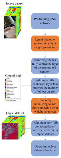
Figure 7.
Hyperspectral image classification process based on deep transfer learning.
5. Optimal Neighborhood Noise-Reduction Method
In order to reduce the salt-and-pepper noise in the initial classification results, an optimal neighborhood noise reduction method based on the eight-neighbor mode label was proposed in this article. The optimal neighborhood noise reduction method was used to reprocess the initial classification result of the hyperspectral image. In the method, the hyperspectral image classification label data was used as the input, and the central pixel label was compared to the label of its eight-neighborhood pixel.
If is used to represent the classification result label of a central pixel of the hyperspectral image, the class labels of the central pixel and the eight neighborhood pixels are shown in Figure 8.
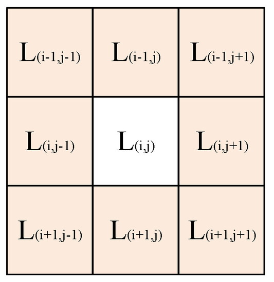
Figure 8.
Class labels of the central pixel and its eight neighborhood pixels.
As shown in Figure 8, based on the traversal of all the pixel labels of the hyperspectral image, the class label of one central pixel and the class labels of the eight neighborhood pixels were combined into a 3×3 matrix. The 3×3 matrix was transformed into a 1×9 one-dimensional vector. Then the mode M of the nine labels and the number m of the mode labels were calculated. The threshold was set to N (0 ≤ N ≤ 9), and the pixel label of the hyperspectral image that did not need to be classified was set to 0. The central pixel is considered to be noise when the following conditions are met: The class label of the central pixel is not equal to the mode of the nine pixel labels, the mode label is not 0, and the number of the mode labels is m ≥ N. Since the label of 0 means that the pixel does not need to be classified, the mode label with the value of 0 is excluded to avoid the edge misjudgment. If the central pixel is confirmed to be noise, it is replaced with the mode label of the eight neighborhood pixels. The initial value of the threshold N is generally set to 5. When the central pixel label is not equal to the mode label of the nine pixels, the mode label is not 0, and the number of the mode labels is m ≥ 5, the central pixel is considered to be noise. The threshold N can be modified according to actual conditions. If the threshold is too large, the noise-reduction effect may not be obvious; if the threshold is too small, the actual information may be misjudged as noise.
The pseudo-code of the optimal neighborhood noise reduction process is shown as follows:
| Input: The classification result dataset X of the hyperspectral image, the label of 0 for the pixels that do not need to be classified, and the threshold N=5 Output: The noise-reduced classification result data set X of the hyperspectral image and classified image with noise reduction. Load classification result dataset X for i=1; i< X.shape[0]; i++ for j=1; j<X.shape[1]; j++ loop traversing each pixel label Transforming the 3×3 matrix composed of the central pixel label L(i,j) and its eight neighborhood pixel labels into a 1×9 one-dimensional vector Calculating the mode M and its number m of central pixel label and the eight neighborhood pixels labels. if the class label of the central pixel is not equal to the mode number M of the nine labels if the mode label is not 0 and the number of the mode label is m≥N The central pixel is noise Replace the central pixel label with the mode label M to remove the noise end if end if Update the hyperspectral image classification result label of each pixel end loop end for end for |
6. Experiments and Analysis
6.1. Dataset
In order to verify the proposed method in this article, the experiments were conducted on the datasets with similar characteristics. The selected dataset included the Indian Pines dataset, the Salinas dataset, the Pavia University dataset, and the Pavia Center dataset. Both the Indian Pines dataset and the Salinas dataset were acquired by AVIRIS sensors. The corrected spectral dimensions for both datasets were 200 and 204, respectively, which were very close. The real ground objects were divided into 16 classes [44]. The Pavia University dataset and the Pavia Center dataset were collected by ROSIS sensors. The corrected spectral dimensions of these two datasets were 103 and 102, respectively, and the real ground objects were divided into nine classes [45]. The datasets are gotten from the website (http://www.ehu.eus/ccwintco/index.php?title=Hyperspectral_Remote_Sensing_Scenes).
The Indian Pines dataset and the Salinas dataset were similar, and the Pavia University dataset and the Pavia Center dataset were similar. In addition, the former two datasets had a smaller sample size than the latter two datasets. Therefore, the Salinas dataset and the Pavia Center dataset were used as the source datasets in the transfer learning method, while the Indian Pines dataset and the Pavia University dataset were used as the corresponding object datasets. First, the structures and parameters of the shallow network were obtained and validated from the training on the Salinas dataset and Pavia Center dataset. Then the obtained structure and parameters were transferred to the Indian Pines dataset and Pavia University dataset with relatively small sample sizes. Finally, the structure and parameters of the network were fine-tuned.
There was a big difference between the Indian Pines dataset and the Pavia University dataset, which could be used to validate the proposed classification method fully. The Indian Pines dataset had a small sample size and can mainly reflect the vegetation information, including rich species and mostly regular block distribution, rich spectral information and low spatial resolution. The Pavia University dataset had a large image size and can mainly reflect the landscape information of the urban landscape. Although there were few species, the shape of the object was irregular, and the spatial resolution was high.
6.2. Experiments and Result Analysis
6.2.1. Experiments of Dimensionality Reduction Methods
In order to test the effectiveness of the proposed methods in the dimensionality reduction and noise reduction for the hyperspectral images, the classification performance of IM, IM_SPE methods, and these methods superimposed with optimal neighborhood noise-reduction method (IM_DN, IM_SPE_DN methods) were tested and compared with that of the spectral information based CNN classification method (SPE) [46], the spatial information based CNN classification method (PCA1, PCA first principal component) [47], the CNN classification method based on the integration of the spectral information and the first principal component of the spatial information (PCA1_SPE), and the CNN classification method based on PCA’s first three principal components of the spectral information (PCA3) [48]. We use OA, AA and Kappa coefficients to evaluate the performance of different methods.
(1) Experiments on Indian pines dataset
The classification performance on the Indian pines dataset is shown in Table 1. From Table 1, for the Indian pines dataset, the PCA1_SPE, PCA3, IM, and IM_SPE classification methods provided the best classification accuracy. Moreover, the OA, AA and Kappa coefficients of IM and IM_SPE methods were superior to those of SPE, PCA1, PCA1_SPE, and PCA3 methods, which indicated that the information measure-based classification method (IM and IM_SPE) had better performance than the spectral information-based classification method (SPE) and the PCA-based classification method (PCA1, PCA1_SPE and PCA3). Among all classification methods, the IM_DN and IM_SPE_DN methods had the best OA, AA, and Kappa coefficients, due to the combination of the dimensionality reduction based on information measure and the optimal neighborhood noise reduction. It has been demonstrated that the optimal neighborhood noise reduction method had a significant effect on the treatment of salt-pepper-noise of the classification results, and can greatly improve the classification accuracy.

Table 1.
The classification results on Indian pines dataset (%).
Figure 9a–i show the classification results of the SPE, PCA1, PCA1_SPE, PCA3, IM, IM_SPE, IM_DN, and IM_SPE_DN methods on the Indian pines data set. Figure 9i shows the ground truth of Indian pines dataset.
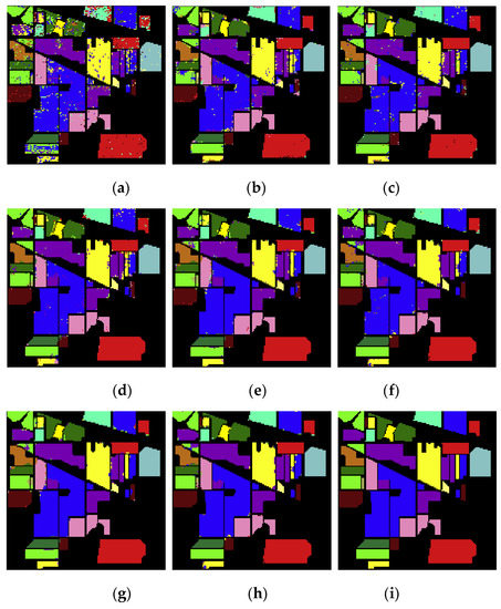
Figure 9.
The classification results on Indian Pines dataset: (a) SPE; (b) PCA1; (c) PCA1_SPE; (d) PCA3; (e) IM; (f) IM_SPE; (g) IM_DN; (h) IM_SPE_DN; (i) the ground truth.
From Figure 9, the classification accuracy of the IM and IM_SPE methods was superior to that of the SPE, PCA1, PCA1_SPE and PCA3 methods on the Indian pines dataset. In addition, the dimensionality reduction method based on information measure played an important role in improving the image classification performance. The salt-pepper-noise of the hyperspectral image was significantly reduced by IM_DN and IM_SPE_DN methods, indicating that the optimal neighborhood noise reduction method can provide a more accurate classification effect.
(2) Experiments on Pavia University dataset
The classification performance of the SPE, PCA1, PCA1_SPE, PCA3, IM, IM_SPE, IM_DN, and IM_SPE_DN methods on the Pavia University data set is shown in Table 2. From Table 2, the OA values of the IM and IM_SPE methods were 6.49% and 7.04% higher than the SPE method on the Pavia University dataset, respectively. Compared with the PCA1 method, the OA values of the IM and IM_SPE methods were increased by 3.76% and 4.31%, respectively. Compared with the spatial-spectral fusion methods (PCA1_SPE and PCA3), the OA values were increased by 0.2%~3.43% and 0.75%~3.98%, respectively. Thus, the spectral selection method based on information measure can significantly improve the classification accuracy. Among all classification methods, the IM_DN and IM_SPE_DN methods, which combined the dimensionality reduction based on the information measure and the optimal neighborhood noise reduction, had the best OA, AA, Kappa coefficients. The AA of IM_SPE_DN method reached as high as 99.20%. Therefore, when the sample size is sufficiently large, the optimal neighborhood noise reduction method can improve the classification performance to a large extent.
Table 2.
The classification results on Pavia University dataset (%).
Figure 10a–i show the classification results of the SPE, PCA1, PCA1_SPE, PCA3, IM, IM_SPE, IM_DN, and IM_SPE_DN methods on the Pavia University data set, and Figure 10i is the ground truth of Pavia University dataset.
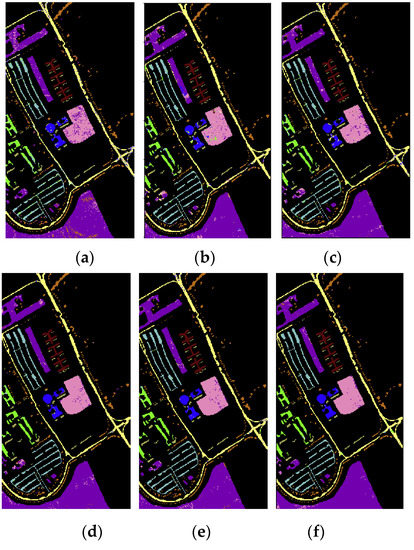
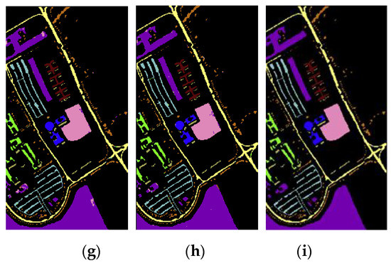
Figure 10.
The classification results on Pavia University dataset: (a) SPE; (b) PCA1; (c) PCA1_SPE; (d) PCA3; (e) IM; (f) IM_SPE; (g) IM_DN; (h) IM_SPE_DN; (i) the ground truth.
As can be seen in Figure 10, it is obvious that the information measure-based CNN classification method (IM and IM_SPE) can achieve higher classification accuracy on the Pavia University dataset. Moreover, the optimal neighborhood noise reduction method (IM_DN and IM_SPE_DN) can effectively reduce the salt-pepper-noise.
The experimental results show that the band selection method based on information measure is better than the feature extraction method based on PCA on Indian pines dataset and Pavia University dataset. As we all know, besides PCA, there are some common dimensionality reduction methods, such as Kernel-PCA (KPCA), independent component correlation (ICA) [49], locally linear embedding (LLE) [50], etc. Research shows that machine learning by feature extraction can achieve better generalization performance than that without feature extraction. This demonstrates the fact that dimensionality reduction can improve generalization performance. Generally speaking, KPCA and ICA perform better than PCA—which is explained by the fact that KPCA and ICA can explore higher order information of the original inputs than PCA. Instead of the sample covariance matrix, (the second-order information) as used in PCA, the negentropy in ICA could take into account the higher order information of the original inputs. By using the kernel method to generalize PCA into nonlinear, KPCA also implicitly takes into account the high order information of the original inputs. A higher number of principal components could also be extracted in KPCA, eventually resulting in the best generalization performance. LLE is much better than PCA in dealing with so-called manifold dimensionality reduction. LLE maps its inputs into a single global coordinate system of lower dimensionality, and its optimizations do not involve local minima. By exploiting the local symmetries of linear reconstructions, LLE is able to learn the global structure of nonlinear manifolds, such as those generated by images of faces or documents of text. So, in the future research, we can try to use KPCA, ICA, LLE to replace the methods based on information measurement, or compare our in this paper with the classification methods based on these dimensionality reduction methods for further experimental testing.
Moreover, entropy and mutual information are used to select the most representative band of the hyperspectral image, in order to reduce the dimension. From the introduction, we can see that some hyperspectral image classification methods based on RBMS or DBN have appeared in the past few years. It is known that Restricted Boltzmann Machines (RBMs) based on unsupervised learning can be used to preprocess the data and basically to help the "machine learning" process become more efficient. Mousas et al. used RBMs to preprocess the motion features of a character’s hand to enhance the estimation rate [51]. Nam et al. used sparse RBM to encode the preprocessed data into high-dimensional feature vectors in the field of music annotation and retrieval [52]. The classification methods based on RBMS or DBN generally take all spectral information of each pixel as the input of the network, and realize the classification of hyperspectral images only according to spectral information. In recent years, some classification methods using spatial-spectral information have achieved better classification results. For feature extraction of the image after dimensionality reduction, the reason why we use CNN instead of RBMS or DBN is that we want to use spatial-spectral information to classify hyperspectral images in order to improve classification accuracy. The validity of this method is also proved by the experiments.
6.2.2. Experiments of Deep Transfer Learning Methods
(1) Transfer experiment from Salinas to Indian pines
Salinas was used as a source dataset to pre-train CNN. Then the shallow layers’ weight parameters were transferred to the object dataset, Indian Pines. In addition, the fine-tuning of the parameters in the network and the optimal neighborhood noise reductions were performed. In this experiment, 5% of the Salinas dataset samples were randomly selected to pre-train CNN, 10% of the Indian Pines dataset were selected as the training set, and the rest of the dataset were used as the test samples.
In order to fully verify the effectiveness of the transfer learning method, the classification method based on all spectrum data of hyperspectral images (that is, No Dimensionality reduction, NDR), the IM method, and the IM_SPE method were combined with the deep transfer learning method (MIG) to obtain the NDR_MIG, IM_MIG, and IM_SPE_MIG methods, respectively. Then the NDR_MIG, IM_MIG, and IM_SPE_MIG methods were compared with the classification methods without transfer (i.e., NDR, IM, IM_SPE). At the same time, in order to further verify the effectiveness of the proposed noise reduction method, NDR_MIG, IM_MIG, IM_SPE_MIG, were combined with the optimal neighborhood noise reduction method (DN) to obtain the NDR_MIG_DN, IM_MIG_DN, and IM_SPE_MIG_DN methods, respectively. The classification result of each method is shown in Table 3.
Table 3.
The classification results on Indian pines (%).
From Table 3, on the Indian Pines dataset, the three classification evaluation indicators (OA, AA, and Kappa coefficients) of the classification methods combined with transfer learning (NDR_MIG, IM_MIG and IM_SPE_MIG) were better than those of the non-transfer learning classification method. Especially, the classification accuracy of the NDR_MIG method was 1.77% higher than that of the NDR method. Among all classification methods, the classification methods combined with transfer learning (IM_MIG, IM_SPE_MIG and NDR_MIG) showed the best OA, AA, and Kappa coefficients. In particular, the classification accuracy of NDR_MIG_DN method was higher than that of the NDR method by 2.73%. The problem of the low classification accuracy, due to the insufficient training samples and serious noise was addressed to some degree.
Figure 11a–i are the classification results of the NDR, IM, IM_SPE, NDR_MIG, IM_MIG, IM_SPE_MIG, NDR_MIG_DN, M_MIG_DN, and IM_SPE_MIG_DN methods on the Indian Pines data set
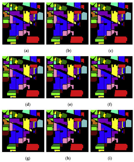
Figure 11.
The classification results on Indian Pines dataset: (a) NDR; (b) IM; (c) IM_SPE; (d) NDR_MIG; (e) IM_MIG; (f) IM_SPE_MIG; (g) NDR_MIG_DN; (h) IM_MIG_DN; (i) IM_SPE_MIG_DN methods.
From Figure 11, it is obvious that the overall classification results on the Indian Pines dataset with small sample size using the classification method with transfer learning are significantly better than those using the classification method without transfer learning. The optimal neighborhood noise reduction method can be used to remove the salt-pepper-noise of the hyperspectral image. Among all the methods, the classification method based on both the deep transfer learning and the optimal neighborhood noise reduction showed the best and most stable classification performance.
(2) Transfer Experiments from Pavia Center to Pavia University
Pavia Center was used as the source dataset to pre-train CNN. Then the weight parameters of the shallow layers were transferred to the object dataset, Pavia University. In addition, the fine-tuning of the network and the optimal neighborhood noise reduction were performed. The Pavia Center and Pavia University datasets were used to represent the datasets with general and sufficient sample sizes, respectively. In the experiment, 9% of the source dataset, Pavia Center samples, were randomly selected to pre-train CNN, 9% of the Pavia University samples were selected as the training set of the object dataset, and the rest samples of the datasets were used as the test samples.
The classification results of the NDR, IM, IM_SPE, IM_MIG, IM_SPE_MIG, NDR_MIG, IM_MIG_DN, IM_SPE_MIG_DN, and NDR_MIG_DN methods on the Pavia University dataset are shown in Table 4.
Table 4.
The classification results on Pavia University (%).
From Table 4, the transfer learning and optimal neighborhood noise reduction methods increased the overall classification accuracy (OA) to above 99% on the Pavia University dataset. In particular, compared with the NDR method, the proposed NDR_MIG and NDR_MIG_DN methods increased the OA by 2.61% and 3.32%, respectively. In addition, the classification and noise-reduction effect of this method was more prominent for the dataset with a larger sample size. The Kappa coefficient of the NDR_MIG_DN method achieved 98.93%, which indicated that almost all the samples were correctly classified based on the consistency check.
Figure 12a–i show the classification results of the NDR, IM, IM_SPE, NDR_MIG, IM_MIG, IM_SPE_MIG, NDR_MIG_DN, M_MIG_DN, and IM_SPE_MIG_DN methods on the Pavia University dataset.
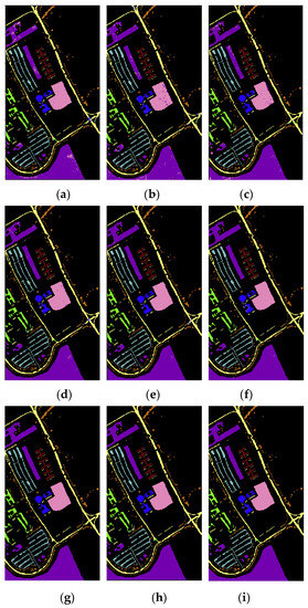
Figure 12.
Classification results on the Pavia University dataset: (a) NDR; (b) IM; (c) IM_SPE; (d) NDR_MIG; (e) IM_MIG; (f) IM_SPE_MIG; (g) NDR_MIG_DN; (h) IM_MIG_DN; (i) IM_SPE_MIG_DN methods.
From Figure 12, the classification method with both the deep transfer learning and the optimal neighborhood noise reduction had outstanding performance on the Pavia University dataset. The classification performance of the proposed classification method with both the deep transfer learning and the optimal neighborhood noise reduction was significantly better than that of the non-transfer learning method (IM, IM_SPE) and NDR). In particular, the hyperspectral images processed by the classification method with both deep transfer learning and optimal neighborhood noise reduction (IM_MIG_DN, IM_SPE_MIG_DN, and NDR_MIG_DN) were almost completely noise-free and correctly classified.
From the above two groups of experiments, i.e., transfer learning classification and neighborhood noise reduction experiments, the classification method based on the transfer learning and neighborhood noise reduction exhibited significant advantages in solving the problem of low classification accuracy under the condition of insufficient training samples, thus, can avoid the over-fitting phenomenon in the training of small CNNs. By transfer between two similar datasets with a large sample size, the computational complexity can be reduced, and the accurate and stable classification results can be obtained. At the same time, through the optimal neighborhood noise reduction, the final classification result was almost noiseless. The results indicated that the transfer learning classification method and the optimal neighborhood noise reduction method could significantly improve the classification performance for the hyperspectral image.
7. Conclusions
In this article, a deep transfer HSI classification method based on information measure and optimal neighborhood noise reduction was proposed. In this method, the information measure was used to reduce the dimension of the hyperspectral image. Then the fusion of the key spectral information and spatial information of the hyperspectral image was achieved, and the redundant spectral information was processed. On this basis, a classification method based on deep transfer learning and neighborhood noise reduction was proposed. The obtained classification accuracy for small samples was higher than 98% on average. Compared with the non-transfer learning method, the total classification accuracy was improved by at least 3%. For the Pavia University dataset with more samples, the classification accuracy of above 99% was obtained. The proposed method can both reduce the computational complexity to some degree and solve the problem of lower classification accuracy caused by insufficient training samples and salt-pepper-noise.
This method is suitable for HSI classification with insufficient training samples. When this situation occurs, we can use labeled samples in similar scenarios to train the network initially, and then adjust the network by transfer learning and a small number of labeled samples to achieve accurate classification of object scenarios. In addition, another advantage of this method is that by dimensionality reduction based on information measure, a pseudo-color image of the hyperspectral image can be obtained, and the hyperspectral image can be visualized. It is worth noting that the core of this method is based on transfer learning, so its limitation is that, at first, we need to get good training on a source scene similar to the target scene, which requires a sufficient number of training samples in the source scene. In the application of constructing a virtual land environment, it is necessary to select some typical scenes for common sensors, mark the samples in these typical scenes, and train the initial network. When constructing the virtual land environment for a specific area in the virtual test, the initial network trained by appropriate scene is selected, and then the high accuracy ground truth of the task area can be obtained by using the proposed method. In this paper, we make the validation by using public datasets. In future work, we will acquire relevant satellite data according to the actual task requirements, and use the proposed method to achieve high-precision ground feature information in the construction of a virtual land environment.
Author Contributions
Conceptualization and methodology, L.L. and C.C.; validation and formal analysis, C.C. and S.Z.; resources, J.Y. and C.C.; writing—original draft preparation, C.C.; writing—review and editing, C.C. and J.Y.; supervision, L.L.
Funding
This work was supported by the National Natural Science Foundation of China (Grant No. 61671170) and National Key R&D Plan (Grant No.2017YFB1302701).
Conflicts of Interest
The authors declare no conflict of interest.
References
- Fang, B.; Li, Y.; Zhang, H.; Chan, J.; Bei, F.; Ying, L.; Haokui, Z. Semi-Supervised Deep Learning Classification for Hyperspectral Image Based on Dual-Strategy Sample Selection. Remote Sens. 2018, 10, 574. [Google Scholar] [CrossRef]
- Lacar, F.M.; Lewis, M.M.; Grierson, I.T. Use of hyperspectral imagery for mapping grape varieties in the Barossa Valley, South Australia IGARSS 2001. Scanning the Present and Resolving the Future. In Proceedings of the IEEE 2001 International Geoscience and Remote Sensing Symposium (Cat. No.01CH37217), Sydney, Australia, 9–13 July 2001. [Google Scholar]
- Mou, L.; Ghamisi, P.; Zhu, X.X. Unsupervised Spectral-Spatial Feature Learning via Deep Residual Conv-Deconv Network for Hyperspectral Image Classification. IEEE Trans. Geosci. Remote Sens. 2018, 99, 1–16. [Google Scholar] [CrossRef]
- Wu, C.; Du, B.; Zhang, L. Slow Feature Analysis for Change Detection in Multispectral Imagery. IEEE Trans. Geosci. Remote Sens. 2014, 52, 2858–2874. [Google Scholar] [CrossRef]
- Hao, W.; Saurabh, P. Convolutional Recurrent Neural Networks for Hyperspectral Data Classification. Remote Sens. 2017, 9, 298. [Google Scholar]
- Nam, J.; Herrera, J.; Slaney, M.; Smith, J.O. Segmentation of white matter hyperintensities using convolutional neural networks with global spatial information in routine clinical brain MRI with none or mild vascular pathology. Comput. Med Imaging Graph. 2018, 66, 28–43. [Google Scholar]
- Krizhevsky, A.; Sutskever, I.; Hinton, G.E. Imagenet classification with deep convolutional neural networks. Adv. Neural Inf. Process. Syst. 2012, 1097–1105. [Google Scholar] [CrossRef]
- Ma, X.; Geng, J.; Wang, H. Hyperspectral image classification via contextual deep learning. Eurasip. J. Image Video Process. 2015, 2015, 20. [Google Scholar] [CrossRef]
- Zhong, Y.; Zhang, L. An Adaptive Artificial Immune Network for Supervised Classification of Multi-/Hyperspectral Remote Sensing Imagery. IEEE Trans. Geosci. Remote Sens. 2012, 50, 894–909. [Google Scholar] [CrossRef]
- Chen, Y.; Lin, Z.; Zhao, X.; Wang, G.; Gu, Y.; Chen, Y.; Lin, Z.; Zhao, X. Deep Learning-Based Classification of Hyperspectral Data. IEEE J. Sel. Top. Appl. Earth Obs. Remote Sens. 2014, 7, 2094–2107. [Google Scholar] [CrossRef]
- Slavkovikj, V.; Verstockt, S.; de Neve, W.; van Hoecke, S.; van de Walle, R.; Slavkovikj, V.; Verstockt, S.; de Neve, W. Hyperspectral image classification with convolutional neural networks. In Proceedings of the 23rd ACM international conference on Multimedia, Brisbane, Australia, 26–30 October 2015. [Google Scholar]
- Makantasis, K.; Karantzalos, K.; Doulamis, A.; Doulamis, N. Deep supervised learning for hyperspectral data classification through convolutional neural networks. In Proceedings of the 2015 IEEE International Geoscience and Remote Sensing Symposium (IGARSS), Milan, Italy, 26–31 July 2015. [Google Scholar]
- Jiang, J.; Ma, J.; Chen, C.; Wang, Z.; Cai, Z.; Wang, L. SuperPCA: A Superpixelwise PCA Approach for Unsupervised Feature Extraction of Hyperspectral Imagery. IEEE Trans. Geosci. Remote Sens. 2018, 1–13. [Google Scholar] [CrossRef]
- Chu, H.S.; Kuo, B.C.; Li, C.H.; Lin, C.T. A semisupervised feature extraction method based on fuzzy-type linear discriminant analysis. In Proceedings of the IEEE International Conference on Fuzzy Systems, Taipei, Taiwan, 27–30 June 2011. [Google Scholar]
- Binliang, J.; Chenglong, F.; Zhaohui, W. Multidimensional scaling used for image classification based on binary partition trees. Comput. Eng. Appl. 2015. [Google Scholar]
- Zhou, X.; Xiang, B.; Zhang, M. Novel Spectral Interval Selection Method Based on Synchronous Two-Dimensional Correlation Spectroscopy. Anal. Lett. 2013, 46, 340–348. [Google Scholar] [CrossRef]
- Jeng-Shyang, P.; Lingping, K.; Sung, P.; Sung, P.W.; Tsai, S.; Vaclav, S. Alpha-Fraction First Strategy for Hierarchical Wireless Sensor Networks. J. Internet Technol. 2018, 19, 1717–1726. [Google Scholar]
- Guo, B.; Gunn, S.R.; Damper, R.I.; Nelson, J.D. Band Selection for Hyperspectral Image Classification Using Mutual Information. IEEE Geosci. Remote Sens. Lett. 2006, 3, 522–526. [Google Scholar] [CrossRef]
- Groves, P.; Bajcsy, P. Methodology for hyperspectral band and classification model selection. In Proceedings of the IEEE Workshop on Advances in Techniques for Analysis of Remotely Sensed Data, Greenbelt, MD, USA, 27–28 October 2003. [Google Scholar]
- Martínez-Usó, A.; Pla, F.; García-Sevilla, P.; Sotoca, J.M. Automatic Band Selection in Multispectral Images Using Mutual Information-Based Clustering. In Proceedings of the Iberoamerican Congress on Pattern Recognition, Cancun, Mexico, 14–17 November 2006; Springer: Berlin/Heidelberg, Germany, 2006. [Google Scholar]
- Wang, B.; Wang, X.; Chen, Z. A hybrid framework for reservoir characterization using fuzzy ranking and an artificial neural network. Comput. Geosci. 2013, 57, 1–10. [Google Scholar] [CrossRef]
- Le Moan, S.; Mansouri, A.; Voisin, Y.; Hardeberg, J.Y. A Constrained Band Selection Method Based on Information Measures for Spectral Image Color Visualization. IEEE Trans. Geosci. Remote Sens. 2011, 49, 5104–5115. [Google Scholar] [CrossRef]
- Salem, M.B.; Ettabaa, K.S.; Bouhlel, M.S. Hyperspectral image feature selection for the fuzzy c-means spatial and spectral clustering. In Proceedings of the 2016 International Image Processing, Applications and Systems (IPAS), Hammamet, Tunisia, 5–7 November 2016. [Google Scholar]
- Hossain, M.A.; Jia, X.; Pickering, M. Subspace Detection Using a Mutual Information Measure for Hyperspectral Image Classification. IEEE Geosci. Remote Sens. Lett. 2014, 2, 424–428. [Google Scholar] [CrossRef]
- Li, W.; Wu, G.; Du, Q. Transferred Deep Learning for Anomaly Detection in Hyperspectral Imagery. IEEE Geosci. Remote Sens. Lett. 2017, 14, 597–601. [Google Scholar] [CrossRef]
- Mehmood, A.; Nasrabadi, N.M. Kernel wavelet-Reed-Xiaoli. An anomaly detection for forward-looking infrared imagery. Appl. Opt. 2011, 50, 2744–2751. [Google Scholar] [CrossRef]
- Yokoya, N.; Iwasaki, A. Object Detection Based on Sparse Representation and Hough Voting for Optical Remote Sensing Imagery. IEEE J. Sel. Top. Appl. Earth Obs. Remote Sens. 2015, 8, 2053–2062. [Google Scholar] [CrossRef]
- Zhang, W.; Teng, S.; Fu, X. Scan attack detection based on distributed cooperative model. In Proceedings of the IEEE International Conference on Computer Supported Cooperative Work in Design, Xi’an, China, 16–18 April 2008. [Google Scholar]
- Wang, J.; Luo, C.; Huang, H.; Zhao, H.; Wang, S. Transferring Pre-Trained Deep CNNs for Remote Scene Classification with General Features Learned from Linear PCA Network. Remote Sens. 2017, 9, 225. [Google Scholar] [CrossRef]
- Wang, L.; Li, J.; Zhou, G.; Yang, D. Application of Deep Transfer Learning in Hyperspectral Image Classification. Comput. Eng. Appl. 2019, 5, 181–186. [Google Scholar] [CrossRef]
- You, S.; Joo, S.G. Virtual Testing and Correlation with Spindle Coupled Full Vehicle Testing System; SAE Technical Paper; SAE International: Thousand Oaks, WA, USA, 2006. [Google Scholar]
- Whyte, J.; Bouchlaghem, N.; Thorpe, A.; McCaffer, R. From CAD to virtual reality: Modelling approaches, data exchange and interactive 3D building design tools. Autom. Constr. 2000, 10, 43–55. [Google Scholar] [CrossRef]
- Bartoldus, K.; Hartung, D.; Eibl, H.; Boehm, J.; Grieb, M.; Pongratz, H. Autonomous Weapons system simulation system for generating and displaying virtual scenarios on board and in flight. U.S. Patent Application 10/413,569, 20 November 2003. [Google Scholar]
- Birkel, P.A. Fall. Synthetic Natural Environment (SNE) Conceptual Reference Model. In Proceedings of the Fall Simulation Interoperability Workshops, Orlando, FL, USA, 14–18 September 1998. [Google Scholar]
- Lyons, D.M. System and Method for Permitting Three-Dimensional Navigation through a Virtual Reality Environment Using Camera-Based Gesture Inputs. U.S. Patent 6,181,343, 30 January 2001. [Google Scholar]
- Arayici, Y. An approach for real world data modelling with the 3D terrestrial laser scanner for built environment. Autom. Constr. 2007, 16, 816–829. [Google Scholar] [CrossRef]
- Chen, F.; Dudhia, J. Coupling an advanced land surface–hydrology model with the Penn State–NCAR MM5 modeling system. Part I: Model implementation and sensitivity. Mon. Weather Rev. 2001, 129, 569–585. [Google Scholar] [CrossRef]
- Throng-The, N.; Jeng-Shyang, P.; Thi-Kien, D. An Improved Flower Pollination Algorithm for Optimizing Layouts of Nodes in Wireless Sensor Network; Digital Object Identifier; IEEE Access: Piscataway, NJ, USA, 2019; Volume 7. [Google Scholar] [CrossRef]
- Shannon, C.E. A Mathematical Theory of Communication. Bell Syst. Tech. J. 1948, 27. [Google Scholar]
- Shaw, M.Q.; Fairchild, M.D. Evaluating the 1931 CIE Color Matching Functions. Res. Appl. 2002, 27, 316–329. [Google Scholar]
- Jacobson, N.P.; Gupta, M.R. Design goals and solutions for display of hyperspectral images. IEEE Trans. Geosci. Remote Sens. 2005, 43, 2684–2692. [Google Scholar] [CrossRef]
- Bell, A.J. The co-information lattice. In Proceedings of the 4th International Symposium on Independent Component Analysis and Blind Signal Separation (ICA2003), Nara, Japan, 1–4 April 2003. [Google Scholar]
- MartÍnez-UsÓMartinez-Uso, A.; Pla, F.; Sotoca, J.M.; García-Sevilla, P. Clustering-Based Hyperspectral Band Selection Using Information Measures. IEEE Trans. Geosci. Remote Sens. 2008, 45, 4158–4171. [Google Scholar] [CrossRef]
- Palmason, J.A.; Benediktsson, J.A.; Sveinsson, J.R.; Chanussot, J. Classification of Hyperspectral Data from Urban areas Using Morphological Preprocessing and Independent Component Analysis; IEEE: Piscataway, NJ, USA, 2005. [Google Scholar]
- Shao, Y.; Sang, N.; Gao, C. Representation Space-Based Discriminative Graph Construction for Semi-supervised Hyperspectral image classification. IEEE Signal Process. Lett. 2017, 25, 1. [Google Scholar]
- Xinyi, S. Hyperspectral Image Classification Based On Convolutional Neural Networks. Master Thesis, Harbin Institute of Technology, Harbin, Heilongjiang, China, July 2016. [Google Scholar]
- Chen, Y.; Jiang, H.; Li, C.; Jia, X.; Ghamisi, P. Deep Feature Extraction and Classification of Hyperspectral Images Based on Convolutional Neural Networks. IEEE Trans. Geosci. Remote Sens. 2016, 54, 6232–6251. [Google Scholar] [CrossRef]
- Lishuan, H. Study of Dimensionality Reduction and Spatial-spectral Method for Classification of Hyperspectral Remote Sensing Image. Ph.D. Thesis, China University of Geosciences, Wuhan, Hubei, China, October 2018. [Google Scholar]
- Cao, L.J.; Chua, K.S.; Chong, W.K.; Lee, H.P.; Gu, Q.M. A comparison of PCA, KPCA and ICA for dimensionality reduction in support vector machine. Neurocomputing 2003, 55, 321–336. [Google Scholar] [CrossRef]
- Roweis, S.T.; Saul, L.K. Nonlinear dimensionality reduction by locally linear embedding. Science 2000, 290, 2323–2326. [Google Scholar] [CrossRef] [PubMed]
- Mousas, C.; Anagnostopoulos, C.N. Learning Motion Features for Example-Based Finger Motion Estimation for Virtual Characters. 3d Res. 2017, 8, 25. [Google Scholar] [CrossRef]
- Nam, J.; Herrera, J.; Slaney, M.; Smith, J.O. Learning Sparse Feature Representations for Music Annotation and Retrieval. In Proceedings of the 13th International Society for Music Information Retrieval Conference, ISMIR 2012, Porto, Portugal, 8–12 October 2012; pp. 565–570. [Google Scholar]
© 2019 by the authors. Licensee MDPI, Basel, Switzerland. This article is an open access article distributed under the terms and conditions of the Creative Commons Attribution (CC BY) license (http://creativecommons.org/licenses/by/4.0/).