1. Introduction
In recent years, convolutional neural networks (CNNs) have gained great success in various computer vision applications such as image classification [
1], object detection [
2], and face recognition [
3]. CNNs have been primarily applied on 2D images to automatically extract spatial features and have significantly enhanced the image classification accuracy. To effectively incorporate the motion information in video analysis, 3D CNNs with spatiotemporal convolutional kernels are proposed. Owing to the ability to capture both spatial and temporal features, 3D CNNs have been proved to be very effective in many video-based applications including object recognition [
4], hand gesture recognition [
5], and human action recognition [
6].
CNNs require vast amounts of memory as there are millions of parameters in a typical CNN model. Meanwhile, CNNs are computationally intensive with over billions of operations for the inference of one input. For example, VGG16 [
7], a real-life 2D CNN model for image classification with 16 layers, takes around 31 GOPs for the inference of one image. C3D [
6], a real-life 3D CNN model for human action recognition with only 11 layers, takes more than 77 GOPs for the inference of a video volume. As a result, CNN applications are mainly run on clusters of server CPUs and GPUs. What is more, with the availability of compatible deep learning frameworks, including Caffe [
8], Theano [
9], and TensorFlow [
10], training and testing CNN models become much easier and more efficient on these platforms. While CPU and GPU clusters are the dominant platforms in CNN applications, customized accelerators with better energy efficiency and less power dissipation are still required. For example, in the case of embedded systems with limited power such as auto-piloted car and robots, higher energy efficiency is critical to increase the use of CNNs.
Owing to the advantages of high performance, energy efficiency, and flexibility, FPGAs have attracted attention to be explored as CNN acceleration platforms. Moreover, high-level synthesis (HLS) tools from FPGA vendors, such as Xilinx Vivado HLS and Intel FPGA SDK for OpenCL, reduce the programming difficulty and shorten the development time significantly, making FPGA-based solutions more popular. As reported in the recent surveys [
11,
12], many FPGA-based CNN accelerators have been proposed for 2D CNNs and many tool-flows for mapping 2D CNNs on FPGAs have been released. However, there are very few studies on accelerating 3D CNNs on FPGAs. Three-D CNNs are far more computationally intensive than 2D CNNs, and generate far more intermediate results during execution as the input is a video volume instead of a single image, causing greater memory capacity and bandwidth demands. In addition, the design space for 3D CNN acceleration is further expanded since the temporal dimension is introduced, making it even difficult to determine the optimal solution. Therefore, current accelerator designs for 2D CNNs are not fit for accelerating 3D CNNs directly. For example, the designs in [
13,
14] adopt customized computation engines to compute 2D convolutions. As there is one more dimension in 3D convolutions, new computation engines are required with this approach. The design in [
15] computes 2D convolutions with the Fast Fourier Transform (FFT) algorithm. This approach is proved to be effective only for large convolutional kernels like
or
and will be less efficient for small convolutional kernels like
or
. Some designs accelerate 2D convolutions by reducing the computational requirements with the Winograd algorithm [
16], and the design in [
17] even extends the Winograd algorithm to adapt to 3D convolutions. However, the Winograd algorithm is very sensitive to the size of convolutional kernels. For convolutional kernels with different size, different transformation matrices are required. Hence, the Winograd algorithm is perfectly suitable for CNN models with uniform-sized convolutional kernels like VGG while not suitable for CNN models with multi-sized convolutional kernels like AlexNet. Another approach is mapping convolutions to matrix multiplication operations, which is typically adopted in CPU and GPU implementations. Refs. [
18,
19] adopt this approach in their accelerator designs for 2D CNNs and implement accelerators on FPGAs using the OpenCL framework. A main concern of this approach is that it introduces high degree of data replications in the input features, which can lead to either inefficiency in storage or complex memory access patterns. Especially, the weight matrix and the feature matrix are both enlarged by a factor of the kernel temporal depth in 3D convolutions, which further lifts the memory requirement.
We analytically find that the computation patterns in 2D and 3D CNNs are very similar. Motivated by this finding, we attempt to design a uniform accelerator architecture for both 2D and 3D CNNs. In the case of FPGA-based clouds, a uniform architecture allows switching of acceleration services without reprogramming the FPGAs. For ASICs, which are not programmable, a uniform architecture expands the applicability of the ASIC. The uniform architecture design is based on the idea of mapping convolutions to matrix multiplication operations. The first challenge comes from the data replications when mapping the input features to the feature matrix. It will introduce multiplied memory access overheads when storing the entire feature matrix off-chip, and will cost a large amount of memory space when storing the entire feature matrix on-chip. We propose an efficient matrix mapping module that avoids data replications by reusing the overlapped data during the sliding of convolutional windows. In addition, the mapping module generates only a tiling (several columns) of the feature matrix on-the-fly instead of generating the entire one before matrix multiplication, which saves on-chip memory consumption. The second challenge is that the weight matrix and feature matrix are enlarged by a factor of the kernel temporal depth in 3D convolutions compared to 2D CNNs. Accordingly, it lifts the memory consumption by a factor of the kernel temporal depth when storing the weight matrix and feature matrix on-chip. To guarantee the uniform architecture can be applied to large CNN models and be deployed on platforms with limited on-chip memory capacity, we adopt an effective splitting strategy. A convolutional layer with a large amount of input channels will be split into multiple convolutional layers with a smaller amount of input channels. The third challenge is how to compute matrix multiplications efficiently on FPGAs. Different to the OpenCL-based computation framework in [
18,
19], we adopt a 2D MAC array for matrix multiplications. The 2D MAC array is scalable and the size is mainly determined according to the hardware resources, memory bandwidth and the size of feature maps.
To summarize, our key contributions are as follows:
We propose a uniform accelerator architecture design supporting both 2D and 3D CNNs, based on the idea of mapping convolutions to matrix multiplication operations. Special efforts are made on memory optimizations and computations to enhance throughput performance;
We analytically model the resource utilization and throughput performance of our architecture, which helps to configure an accelerator on a specific platform within certain constraints including hardware performance, memory bandwidth and clock frequency;
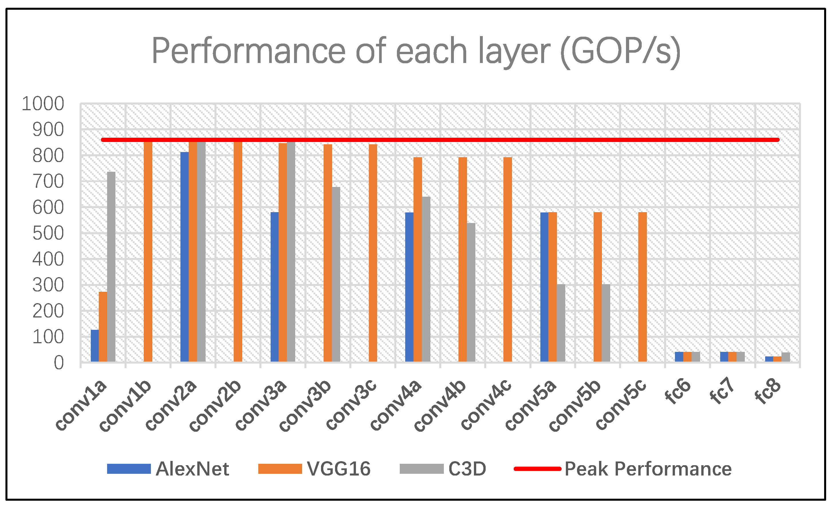
We demonstrate the architecture design by implementing an accelerator on the Xilinx VC709 board with the High-level synthesis (HLS) methodology. Three typical CNN models including AlexNet, VGG16, and C3D, are tested on the accelerator. Experimental results show that the accelerator achieves over 850 GOP/s for convolutional layers and nearly 700 GOP/s overall on VGG16 and C3D, with much better energy efficiency than the CPU and GPU.
The rest of the paper is organized as follows:
Section 2 briefly introduces the basic background of CNNs and the design directions of the accelerator architecture;
Section 3 presents the architecture design and the main components;
Section 4 provides the implementation and optimization details;
Section 5 presents the accelerator modeling;
Section 6 reports the experimental results; and finally,
Section 7 concludes the paper.
2. CNN Basics and Accelerator Design Directions
In this section, we briefly review the operations in convolutional layers of 2D and 3D CNNs and then the accelerator design directions on FPGAs are introduced. The fully-connected layers, activation, and pooling layers are omitted due to their relative simplicity.
2.1. Operations in Convolutional Layers of 2D CNNs
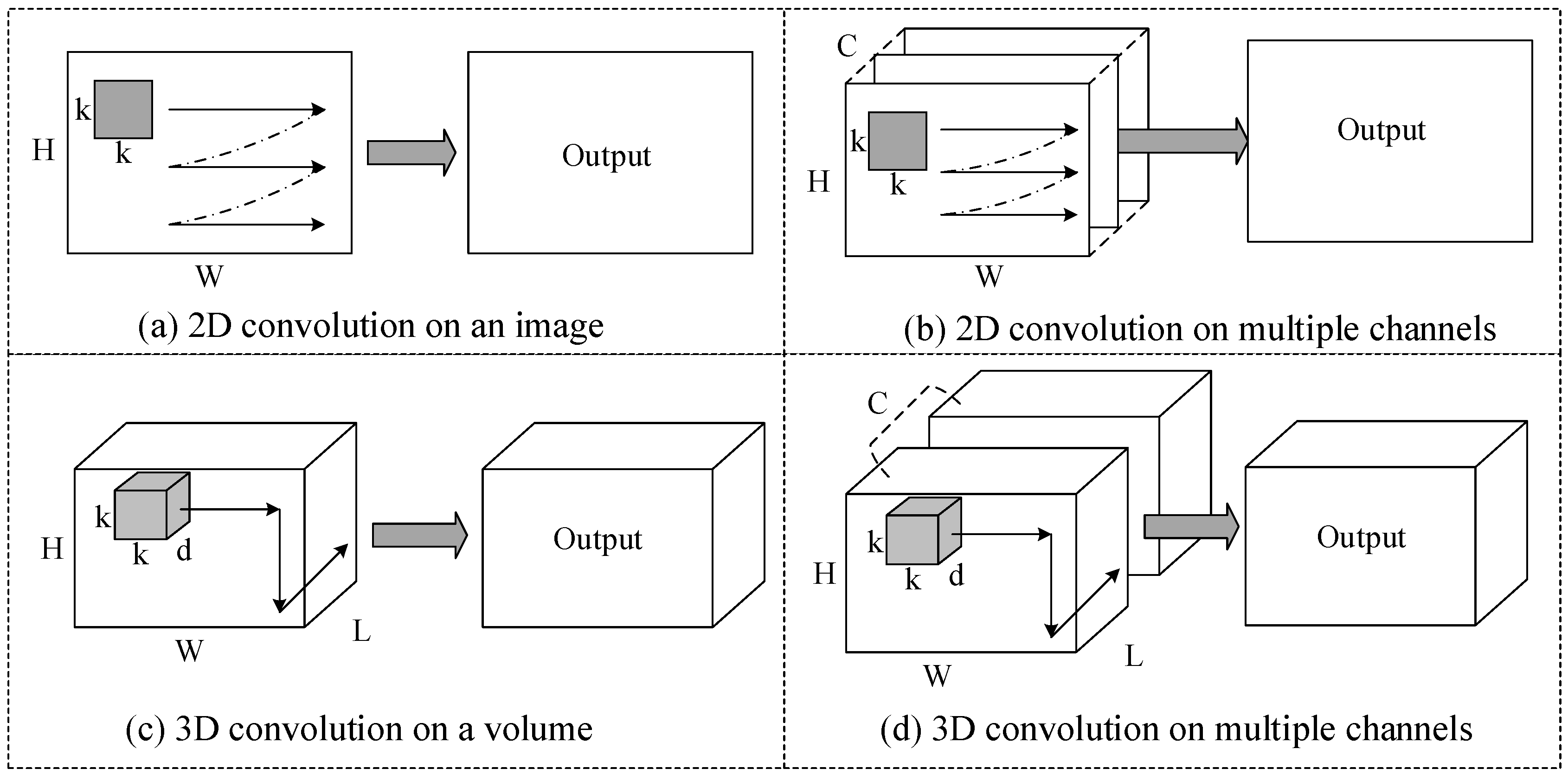
Figure 1a illustrates the process of a 2D convolution. A 2D convolution applied to an image results in another image. In convolutional layers of 2D CNNs, the input and output features are images with multiple channels. For example, the input feature of the first convolutional layer has three channels: Red, green, and blue. A 2D convolution is applied to each channel of the input feature and the generated images are then accumulated resulting in one channel of the output feature, as shown in
Figure 1b. For simplicity, we use
X to indicate the input feature with a size of
and
Y to indicate the output feature with a size of
. Here,
c and
m are the number of input and output channels, and
h and
w are height and width of each feature. We use
W to indicate the weights, which contains
kernels with a size of
. Suppose the sliding stride is 1, then each pixel
in the output feature is calculated by:
2.2. Operations in Convolutional Layers of 3D CNNs
Figure 1c illustrates the process of a 3D convolution. A 3D convolution applied to a video volume results in another volume. Similarly, in convolutional layers of 3D CNNs, the input and output features are video volumes with multiple channels. A 3D convolution is applied to each channel of the input feature and the generated volumes are then accumulated resulting in one channel of the output feature, as shown in
Figure 1d. The input and output features are indicated by
X with a size of
and
Y with a size of
, where
l is the number of frames while the other variables have the same meaning as above. The weights
W contains a total of
kernels with a size of
, where
d is the kernel temporal depth and
k is the kernel spatial size. Suppose the sliding stride is 1, then each pixel
in the output feature is given by:
Compared to the convolutional layers in 2D CNNs, there is an accumulation along the temporal dimension, as shown in Equation (
2). By switching the order of the two outer accumulations, we get Equation (
3). We can find that the inner three accumulations in Equation (
3) are very similar to Equation (
1) since the loop variable along the temporal dimension
is fixed.
We can further combine the outer two loops and hence get Equation (
4), which is almost the same as Equation (
1) except that the number of input channels is enlarged by a factor of
d. That is to say, 3D convolutions can be computed in the same way as 2D convolutions.
2.3. Convolution as Matrix Multiplication
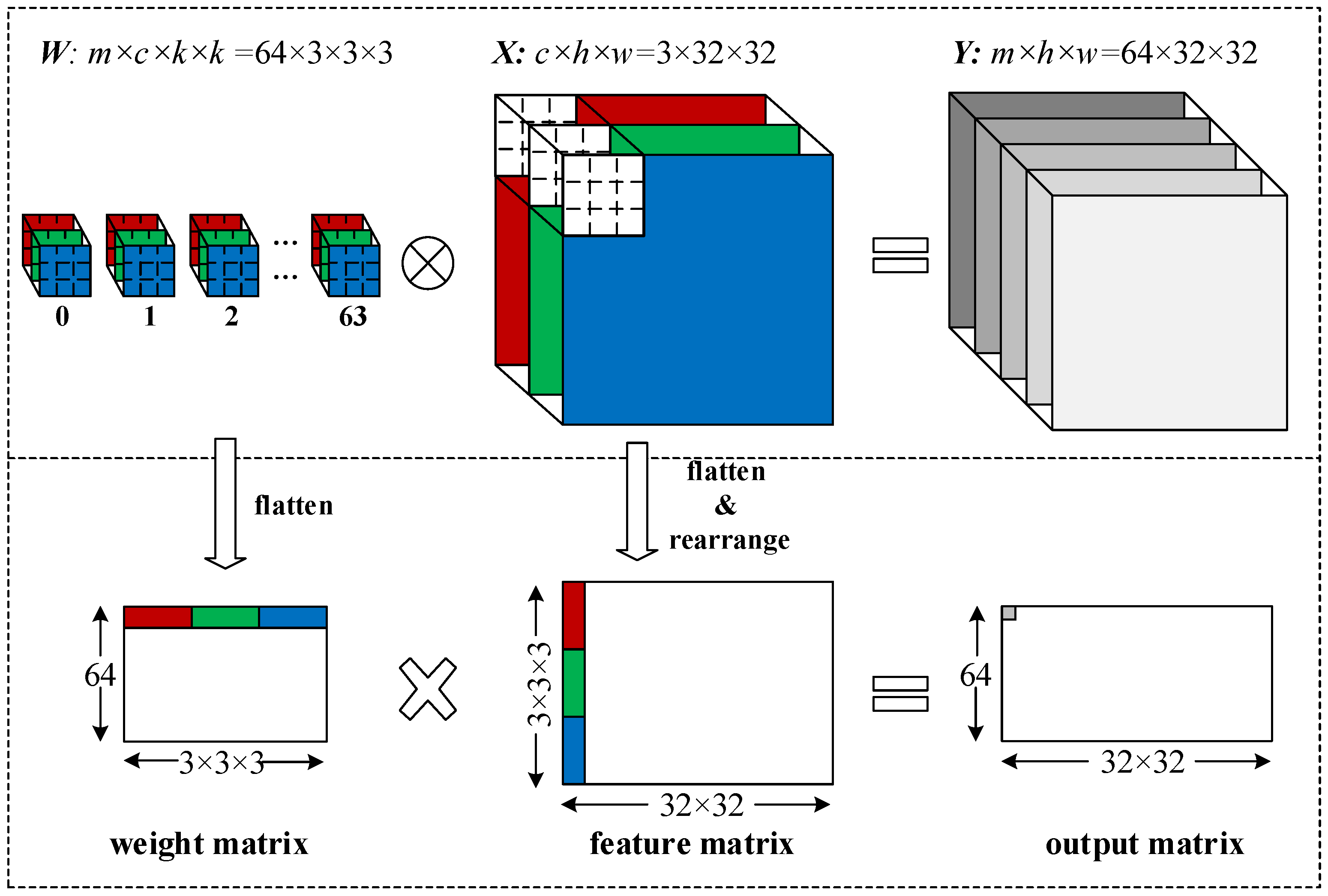
Two-D convolutions can be mapped as matrix multiplication operations by flattening and rearranging the weights and input features. As illustrated in
Figure 2,
kernels with a size of
are mapped to a rearranged matrix with dimensions of
. All three kernels belonging to the same group are flattened horizontally to form a row of the weight matrix. Meanwhile, all three input features with dimensions of
are mapped to a rearranged matrix with dimensions of
. All the pixels covered by the first convolution window in each channel are flattened vertically to form the first column of the feature matrix. The entire feature matrix can be generated by sliding the convolution window across the features along the column and row directions. After rearrangement, the convolutions are transformed to a general matrix multiplication. The result of the matrix multiplication is an output matrix with dimensions of
, which is the flattened format of the output features. Notice that the number of the pixels in the feature matrix is (
)-fold to that in the input feature, as each pixel is covered by the convolution window
times during sliding the convolution window across the features and hence replicated
times.
Similarly, 3D convolutions can also be mapped as matrix multiplications with the same method. Compared to 2D convolutions, the convolution window slides across the input features not only along the row and column directions, but also the temporal direction. Consequently, each pixel is covered by the convolution window times and hence replicated times. The number of pixels in the input feature is enlarged by a factor of .
Here we can find that the approach of mapping convolutions as matrix multiplication operations introduces a high degree of data replications. In CPU and GPU implementations, the entire feature matrix is generated first before computing matrix multiplication. This is not a big problem to CPUs and GPUs as they have abundant memory space and bandwidth. However, to FPGAs with limited on-chip memory capacity and off-chip memory bandwidth, storing the entire feature matrix can be a critical limitation. We will show how we optimize this approach in FPGA implementations with a customized matrix mapping module in the next section.
2.4. Splitting Strategy
As shown in
Figure 2, all channels of the input feature are involved to generate one column of the feature matrix. When loading the required pixels of the input feature from off-chip memory to on-chip memory, the burst access pattern is typically adopted to lift memory bandwidth utilization rate. That is to say, we have to store at least several rows for each input channel of the input feature on-chip. In a convolutional layer of a large-scale 2D CNN model, the number of input channels may be very large, 512 or even 1024, which will consume plenty of on-chip memory space. This can be even more severe for a 3D CNN model as the number of input channels is enlarged by a factor of
d. Considering that the target hardware platform may have very limited on-chip memory, we adopt a splitting strategy that splits a convolutional layer with a large number of input channels to multiple convolutional layers with a smaller number of input channels. An independent sum layer is introduced to accumulate the results of two convolutional layers. Suppose the on-chip memory can store at most
input channels, then a convolutional layer with
c input channels will be split into
convolutional layers with
input channels each. Additionally,
sum layers will be introduced to accumulate the partial results. The splitting strategy is a kind of matrix blocking or partitioning method in essence. Different to block matrix multiplication, an independent sum layer is introduced which eliminates the need to store intermediate results on-chip and hence saves on-chip memory consumption.
3. Hardware Architecture Design
We propose a uniform architecture design for accelerating both 2D and 3D CNNs based on the idea of mapping convolutions to matrix multiplication operations. The architecture can adapt to convolutional layers with different input dimensions and kernel sizes, and can support large-scale CNN models owing to the splitting strategy. In this section, the details of the customized matrix mapping module, the computation framework, the buffers, and the whole architecture will be presented.
3.1. Matrix Mapping Module
As introduced above, the approach of mapping convolutions as matrix multiplication operations introduces a high degree of data replications, which will lift the memory access overheads when storing the entire feature matrix off-chip. We propose a customized matrix mapping module that avoids data replications by reusing the overlapped data during the sliding of convolutional windows.
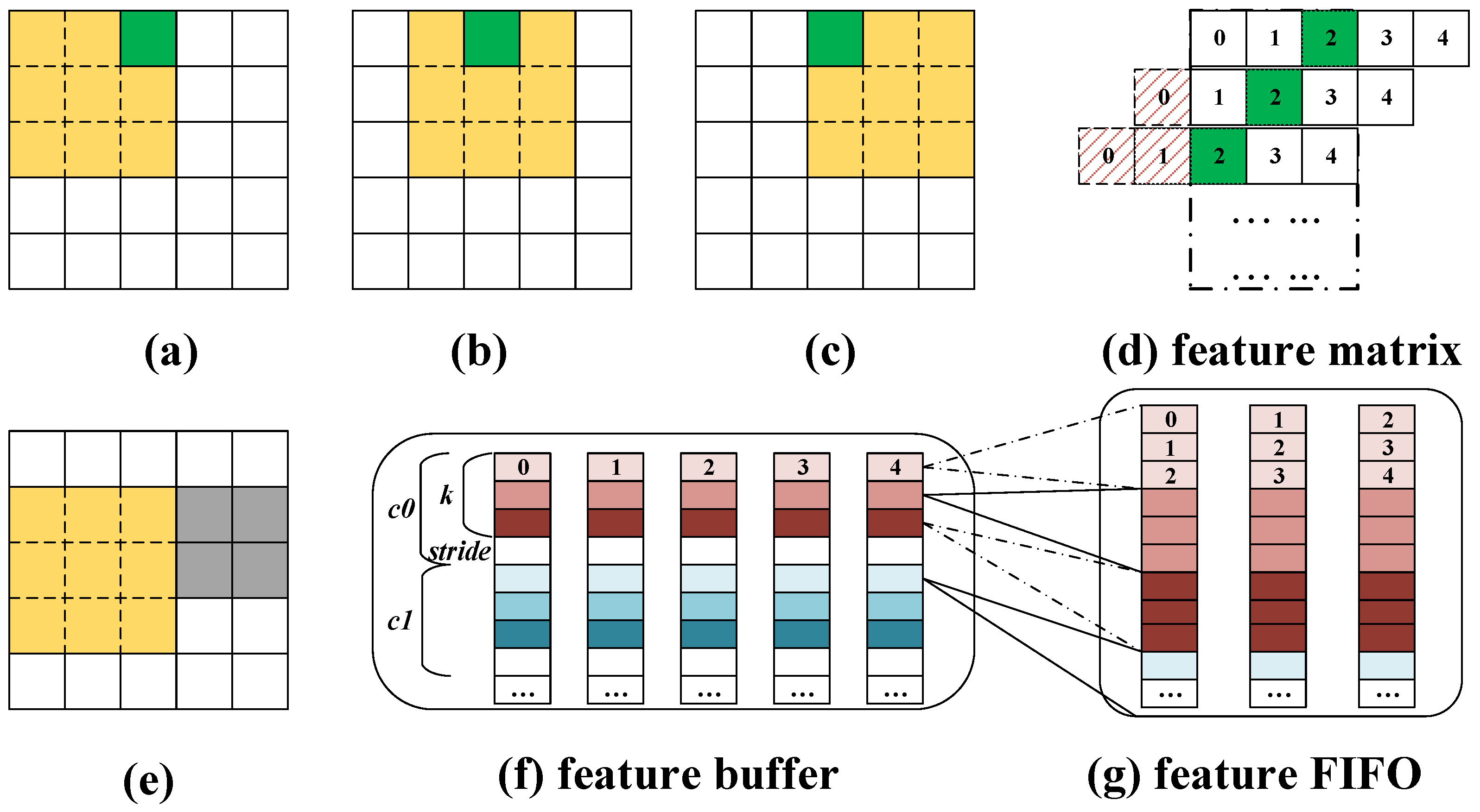
Figure 3a–c illustrate how the convolution window slides across columns of the input feature. The pixel in green is involved in
k convolutions. Accordingly, it appears in the feature matrix
k times in
k consecutive rows. We can generate
k rows of data in the feature matrix by simply shifting the related row in the input feature
k times, as illustrated in
Figure 3d.
Figure 3e shows the status after the convolution window slides vertically across the rows. There are
overlapped rows between two consecutive slides across the rows, which can be reused when the convolution window slides across the columns. Therefore, each pixel is used
times during the process.
To save on-chip memory consumption, we store only
rows for each channel of the input feature (
in most cases) instead of the entire input feature. The first
k rows are for the activated data involved in current convolutions while the left
rows are pre-cached for the next slide across the rows. We partition the input feature by the column dimension to provide enough data ports for data shifting, as shown in
Figure 3f. The matrix mapping module loads
k rows of each channel at the beginning, shifts each row
k times to generate
rows, and writes the feature matrix block to the feature FIFOs, as illustrated in
Figure 3g. Then the matrix multiplication starts and calculates the first row of the output feature. During the process of matrix multiplication, the next
rows in each channel of the input feature will be loaded and replace
rows of data in the same channel according to the First-In-First-Out policy. The process repeats until all the pixels in the output feature are calculated.
3.2. 2D MAC Array
If
A and
B are matrices with dimensions of
and
respectively, then the product matrix
C is given by:
We adopt a 2D MAC array to compute matrix multiplication in the most straightforward way. A MAC unit is composed of a multiplier to calculate the products, an adder to accumulate the products, and a register to keep the partial sum. The MAC unit located at
receives operands from the
i-th row of matrix
A and
j-th column of matrix
B and generates the pixel
. In the case of CNN accelerations,
A is the weight matrix,
B is the feature matrix, and
C is the output matrix. Suppose there are
rows and
columns in the MAC array, then a total of
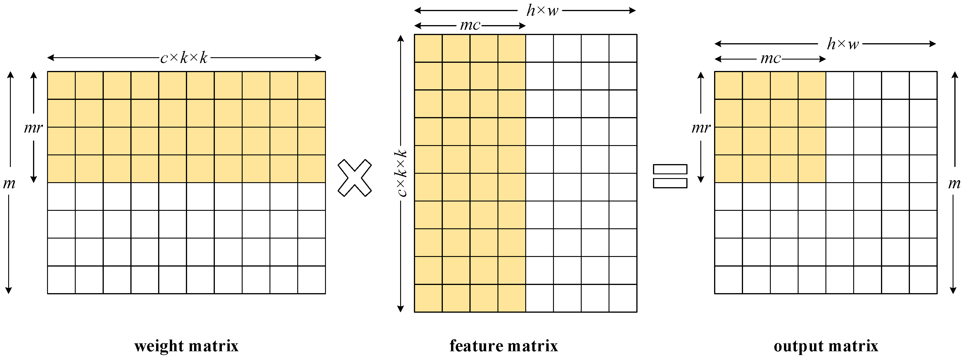
pixels can be generated at once. We adopt a simple matrix partitioning strategy to compute the whole output matrix with the 2D MAC array. As shown in
Figure 4, the weight matrix is partitioned into
matrix blocks along the row dimension and the feature matrix is partitioned into
matrix blocks along the column dimension.
The 2D MAC array exploits the parallelism of convolutions in two aspects. The output channel loop is unrolled by a factor of and hence channels of the output feature can be calculated simultaneously. The column loop of each channel is unrolled by a factor of and thus pixels in the same row of a channel can be computed in parallel. The 2D MAC array is scalable and the size is determined according to the hardware resources, memory bandwidth, feature size and the number of input channels. Hardware resources, especially the DSP slices on a FPGA chip, determine the maximum number of MAC units that can be assigned to the 2D MAC array. The width of the 2D MAC array is mainly restricted by the memory bandwidth. We can find an optimal value for the width so that the 2D MAC array is well matched with the memory bandwidth. The 2D MAC array will be under-utilized when the real width is greater than the optimal value, and the memory bandwidth is not fully exploited when the real width is less than the optimal value. Also, the width of the 2D MAC array is closely related to the feature size of a CNN model. For example, if the feature size is , it is better to deploy 28 columns of MAC units instead of 32, which achieves the same throughput performance with fewer MAC units. The height of the 2D MAC array is closely related to the number of output channels in a CNN model. A common divisor of all the output channel numbers in all convolutional layers is most preferred. A power of two may also be a good choice for the height of the 2D MAC array.
3.3. Buffer Settings
As shown in
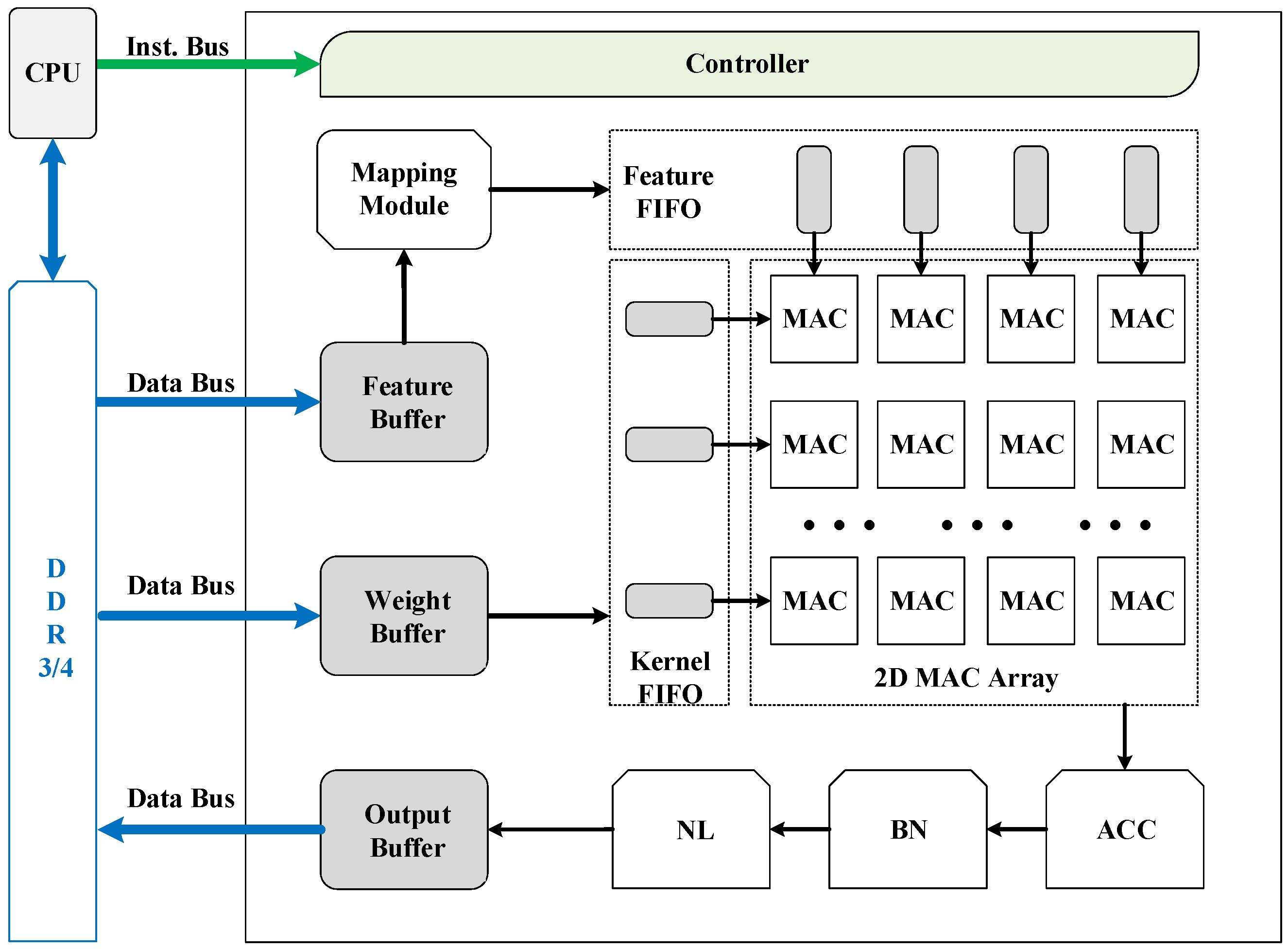
Figure 5, we deploy three buffers for caching data on-chip: The weight buffer for kernels in convolutional layers and weights in fully connected layers, the feature buffer for input features and the output buffer for output features. Each buffer is composed of multiple independent Block RAMs and the number of Block RAMs is carefully selected to perfectly match the needs of the 2D MAC array.
During the process of matrix multiplication, rows of kernel data and columns of feature data are required at every cycle. To offer enough data ports to the 2D MAC array, we assign Block RAMs in the weight buffer and Block RAMs in the feature buffer. The additional Block RAMs are for the padding data when the convolution window slides to the edges. As the 2D MAC array calculates pixels of the output feature simultaneously, we assign Block RAMs in the output buffer. Once the results are generated, they will be cached in the output buffer in cycles, which is much shorter than the matrix multiplication latency. Meanwhile, we can adopt the burst access pattern when storing the output feature back to the off-chip memory, which lifts the memory bandwidth utilization rate.
To save on-chip memory consumption, the weight buffer stores only groups of kernels on-chip, the feature buffer stores rows for each channel of the input feature, and the output buffer stores only rows (one row for each channel) of the output feature. To achieve pipelining between memory access and computation, the input buffer pre-caches rows for each channel of the input feature during the matrix multiplication and the ping-pong strategy is used on the output buffer. Therefore, the memory access time is overlapped with the computation time to the most extent.
3.4. Accelerator Architecture
Figure 5 shows an overview of the uniform accelerator architecture for 2D and 3D CNNs. The major components include a controller for fetching instructions and orchestrating all other modules during executing instructions, three buffers for caching input features, weights, and output features respectively, a mapping module to flatten and rearrange input features to feature matrices, and a 2D MAC array to compute matrix multiplications. There are some supplementary function units: The ACC unit for accumulations of two convolutional layers, the BN unit for batch-norm and scale layers, the NL unit for nonlinear activation functions, and some FIFOs for matrix dataflow during computing matrix multiplications. All buffers are connected through data buses to external DDR3/4 memory. The input features and weights are initialized to the DDR memory by the host CPU, which can be a server CPU or an embedded processor depending on the application scenario.
Given an implemented accelerator, a specific CNN model is computed layer-by-layer by a sequence of macro-instructions. The instructions are fed to the controller directly by the host CPU through the instruction bus.
Table 1 lists all the macro-instructions used in our architecture. Basically, each instruction is corresponding to a layer type in CNNs. A sum layer is specially introduced due to the splitting strategy. In the case when the input feature of a convolutional layer has too many input channels to be stored in the feature buffer, the convolutional layer will be split into multiple convolutional layers with less input channels. Sum layers are then used to accumulate the results of these convolutional layers. The batch-norm, scale, and ReLu layer can be combined with the convolutional or fully-connected layers ahead so no independent instructions are for them. As shown in
Table 2, each macro-instruction is 128-bits long, including the opcode that indicates the layer type, and a series of parameters listed below. The meaning of the left parameters are the same as above.
, the height of the input feature;
, the height of the output feature;
, the number of weight matrix blocks;
, the number of feature matrix blocks;
, the number of padding rows and padding columns;
, option indicating whether there are batch normalization and scale operations;
, option indicating whether there is non-linear function;
4. Accelerator Implementation
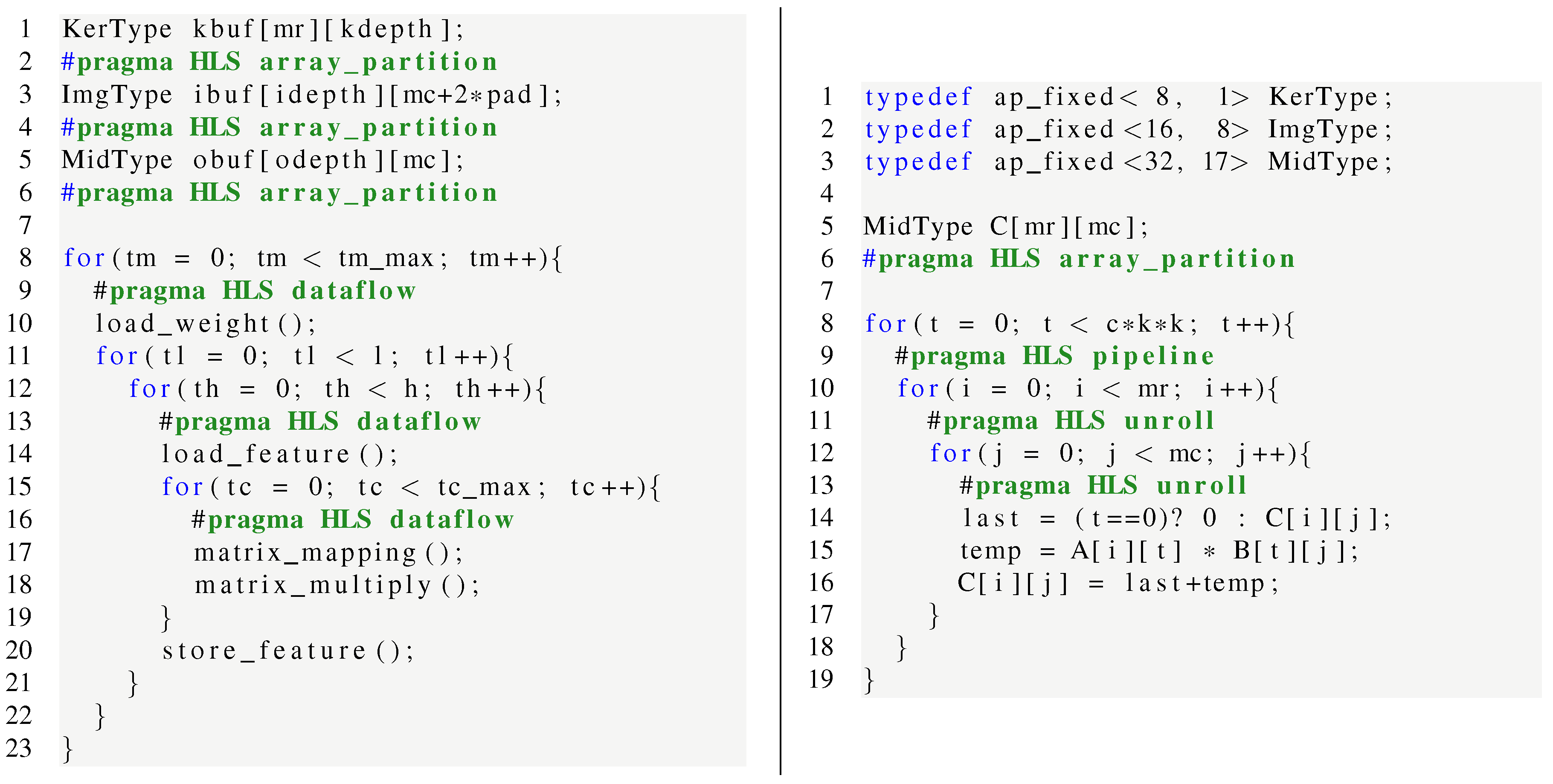
As a case study, we implement an accelerator prototype based on the uniform architecture with the HLS methodology. The pseudo-code in
Figure 6 (left) demonstrates the working process of a convolutional layer. The weight buffer, feature buffer, and output buffer are declared respectively with specified data types. We adopt fixed-point arithmetic logic units in our implementation. As shown in
Figure 6 (right), each kernel is represented by eight bits including one sign bit and seven fraction bits, each pixel in input and output features is represented by 16 bits including one sign bit, seven integer bits, and eight fraction bits, and each intermediate result is represented by 32 bits including one sign bit, 16 integer bits, and 15 fraction bits. The intermediate results are represented by 32 bits to preserve precision during accumulations and will be truncated to 16 bits before writing back to memory. The weight buffer is completely partitioned in the row dimension with the
array_partition pragma. The feature buffer and output buffer are completely partitioned in the column dimension. The core functions include the load-weight function (line 10), the load-feature function (line 14), the matrix-mapping function (line 17), the matrix-multiply function (line 18), and the store-feature function (line 20). As the function name reflects, the load-weight function loads weights from the off-chip memory to the weight buffer; the load-feature function loads the input feature from the off-chip memory to the input buffer; the store-feature function stores the output feature from the output buffer back to the off-chip memory; the matrix-mapping function is corresponding to the matrix mapping module; and the matrix-multiply function is corresponding to the 2D MAC array.
4.1. Computation Optimization with HLS Pragmas
The
dataflow optimization is adopted to improve the throughput performance. The
dataflow pragma enables task-level pipelining, allowing functions and loops to overlap in their operation, and increasing the concurrency of the RTL implementation. As shown in
Figure 6 (left), the
dataflow pragma is specified within the tc-loop, th-loop and tm-loop respectively.
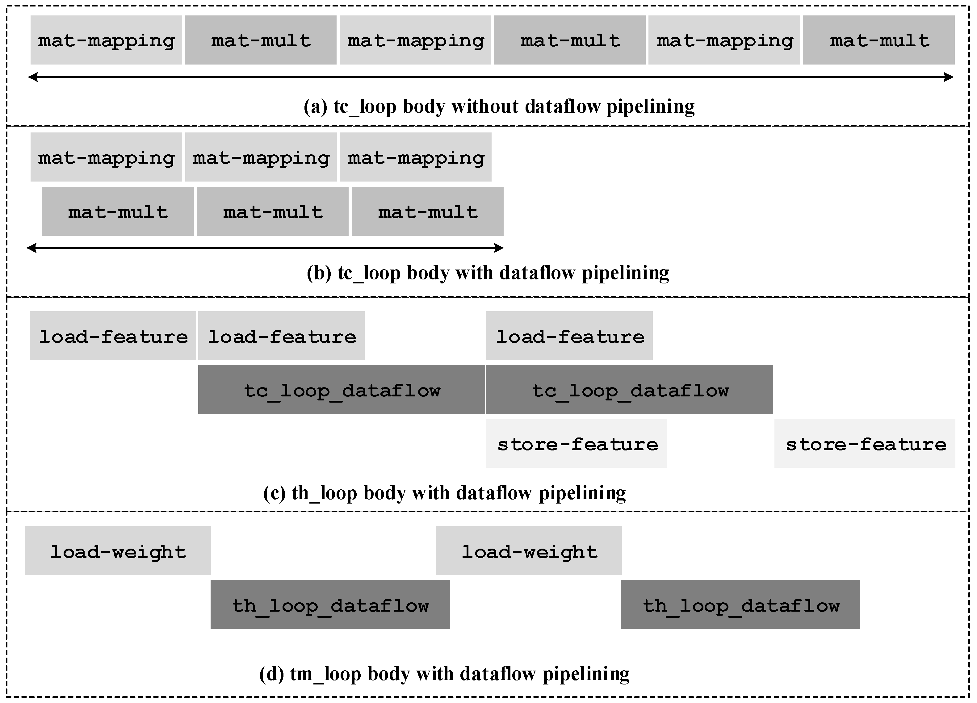
Figure 7a illustrates the working process of the tc-loop without dataflow pipelining. The matrix-mapping function and the matrix-multiply function are processed sequentially. With dataflow pipelining, the matrix-multiply function can begin several cycles after the matrix-mapping function begins, and are almost completely overlapped with the matrix-mapping function, as illustrated in
Figure 7b. Therefore, the latency of the tc-loop with dataflow pipelining is shortened significantly.
Figure 7c shows how the dataflow optimization works on the th-loop. The load-feature function and the store-feature function are fully overlapped by the tc-loop. The th-loop is pipelined and the pipeline interval equals to the maximum latency of the three parts.
Figure 7d illustrates the tm-loop with dataflow pipelining. Notice that the matrix-multiply function is dependent to the weight matrix and hence the th-loop has to wait until the load-weight function is done. The latency of the th-loop is typically much longer than the latency of the load-weight function. For example, in the second convolutional layer of the C3D model, the th-loop takes 37,355 cycles while the load-weight function takes only 578 cycles. In this case, the ping-pong strategy can reduce the execution time by at most
. Therefore, the ping-pong strategy is not adopted on the weight buffer to save on-chip memory consumption. That is why the load-weight function is not fully overlapped with the th-loop.
The HLS pragmas
unroll and
pipeline are used inside these functions to reduce latency and enhance throughput performance.
Figure 6 (right) shows the HLS pseudocode of the matrix-multiply function. The
unroll pragma enables some or all loop iterations to occur in parallel by creating multiple copies of the loop body in the RTL design. In the matrix-multiply function,
multipliers and adders are created shaping the 2D MAC array and hence
multiply-accumulations are computed concurrently. The
pipeline pragma helps to reduce the initiation interval for a loop by allowing the concurrent execution of operations. The initiation interval in the matrix-multiply function is one cycle after optimization. To summarize, the total execution latency is greatly reduced and the system throughput is enhanced significantly owing to the HLS pragmas.
4.2. Memory Optimization
Memory optimizations are made to better use the external memory bandwidth. We expand the data access width using the HLS data_pack pragma, which packs the data fields of a struct into a single scalar with larger byte length. The data_pack pragma helps to reduce the memory access time and all members of the struct can be read and written simultaneously. In our implementation, weights are packed to a for the load-weight function, pixels are packed for the load-feature function, and pixels are packed for the store-feature function.
In addition, we optimize the storage pattern of the features in the external memory space. Since the load-feature function loads one entire row of all input channels every time, the store-feature function stores the features back to the off-chip memory according to the frame-height-channel-width order instead of the frame-channel-height-width order. Therefore, the load-feature function and the store-feature function can transfer data between the on-chip buffer and the off-chip memory in a burst access mode, which lifts the bandwidth utilization rate significantly. The original map is still stored according to the frame-channel-height-width order as we do not want introduce additional work. The large width of the original map guarantees the burst access length in the load-feature function of the first convolutional layer. With the above memory optimizations, the memory bandwidth is no longer the bottleneck. In our implementation, the load-feature and store-feature functions are fully overlapped by the matrix-multiply function. That is to say, the 2D MAC array is only idle during setting up and flushing the pipeline, and will be fully utilized once the pipeline is ready in convolutional layers.
5. Accelerator Modeling
5.1. Resource Modeling
An FPGA has several different types of resources of which DSP slices and on-chip memory (Block RAM) have the most effect on the configuration of a CNN accelerator. Since we are using fixed-point arithmetic in our architecture, the only component that consumes DSP slices is the multiplier in the MAC units. Each multiplier consumes one DSP slice. Hence, the total consumption of DSP slices is given by , which should be less than the total number of available DSP slices.
In terms of on-chip memory utilization, we analytically model the consumption of the weight buffer, input buffer and output buffer. There are
Block RAMs in the weight buffer. Each weight is represented as one byte and hence the width of each Block RAM is 8. Assuming the depth of each Block RAM is
, the total on-chip memory consumed by the weight buffer is
bytes. The depth of each Block RAM is given by Equation (
6) if the on-chip memory is abundant. The
in the equation indicates the total number of layers in a CNN model.
The feature buffer stores input features in
Block RAMs. The additional
Block RAMs are introduced due to the padding required at the edges. Each pixel in input features is represented as two bytes and hence the width of each Block RAM is 16. Assuming the depth of each Block RAM is
, the total on-chip memory consumed by the input buffer can be calculated by
bytes. The depth of each Block RAM is given by Equation (
7) if the on-chip memory is abundant.
In the case when the on-chip memory is limited, and are specified by users under the memory constraint. For some convolutional layers with a large number of input channels, may be less than the width of the weight matrix or may be less than the height of the feature matrix. The splitting strategy will split the convolutional layer to multiple convolutional layers with less number of input channels to fit to the weight buffer and feature buffer.
The output buffer stores output features in
Block RAMs. The ping-pong strategy is adopted for the output buffer. Each pixel in output features is represented as two bytes and hence the width of each Block RAM is 16. Assuming the depth of each Block RAM is
, the total on-chip memory consumed by the output buffer can be calculated by
bytes. The depth of each Block RAM is given by Equation (
8) if the on-chip memory is abundant.
In the case when the on-chip memory is limited or the feature width is too large,
can be specified by users under the memory constraint. The 2D MAC array may be under-utilized in some convolutional layers with large feature width. The real unrolling factor of the output channel loop is less than
, which is given by the following equation:
5.2. Performance Modeling
The main operations in matrix multiplication are multiplications and additions, conducted by the 2D MAC array. As there are MAC units, operations are processed every clock cycle in the ideal case. Therefore, the peak throughput is given by OP/s, where f is the clock frequency.
The actual throughput is the total operations divided by the total execution time. The total operations in a convolutional layer can be calculated by Equation (
10). In 2D convolutional layers,
and
.
Owing to the
dataflow optimization, the functions are working in a pipelined way and some functions are even completely overlapped by others, as illustrated in
Figure 7. The total execution cycles for a convolutional layer can be calculated by Equation (
11) where
,
, and
indicate the execution cycles of the load-weight, load-feature and store-feature function respectively.
indicates the pipeline interval of the th-loop in
Figure 6.
The matrix-mapping function takes
cycles to generate a feature matrix block and the matrix-multiply function also takes
cycles to complete a matrix multiplication. Hence, the total cycles taken by the tc-loop in
Figure 6 is given by:
The execution time of the other functions are closely related to the real memory access bandwidth. We get simplified models for the memory-related functions under sufficient memory access bandwidth: The load-weight function takes cycles, the load-feature function takes cycles, and the store-feature function takes cycles. The pipeline interval of the th-loop is the maximum value of , and .


