A Fusion Frequency Feature Extraction Method for Underwater Acoustic Signal Based on Variational Mode Decomposition, Duffing Chaotic Oscillator and a Kind of Permutation Entropy


Abstract
:1. Introduction
2. Theory
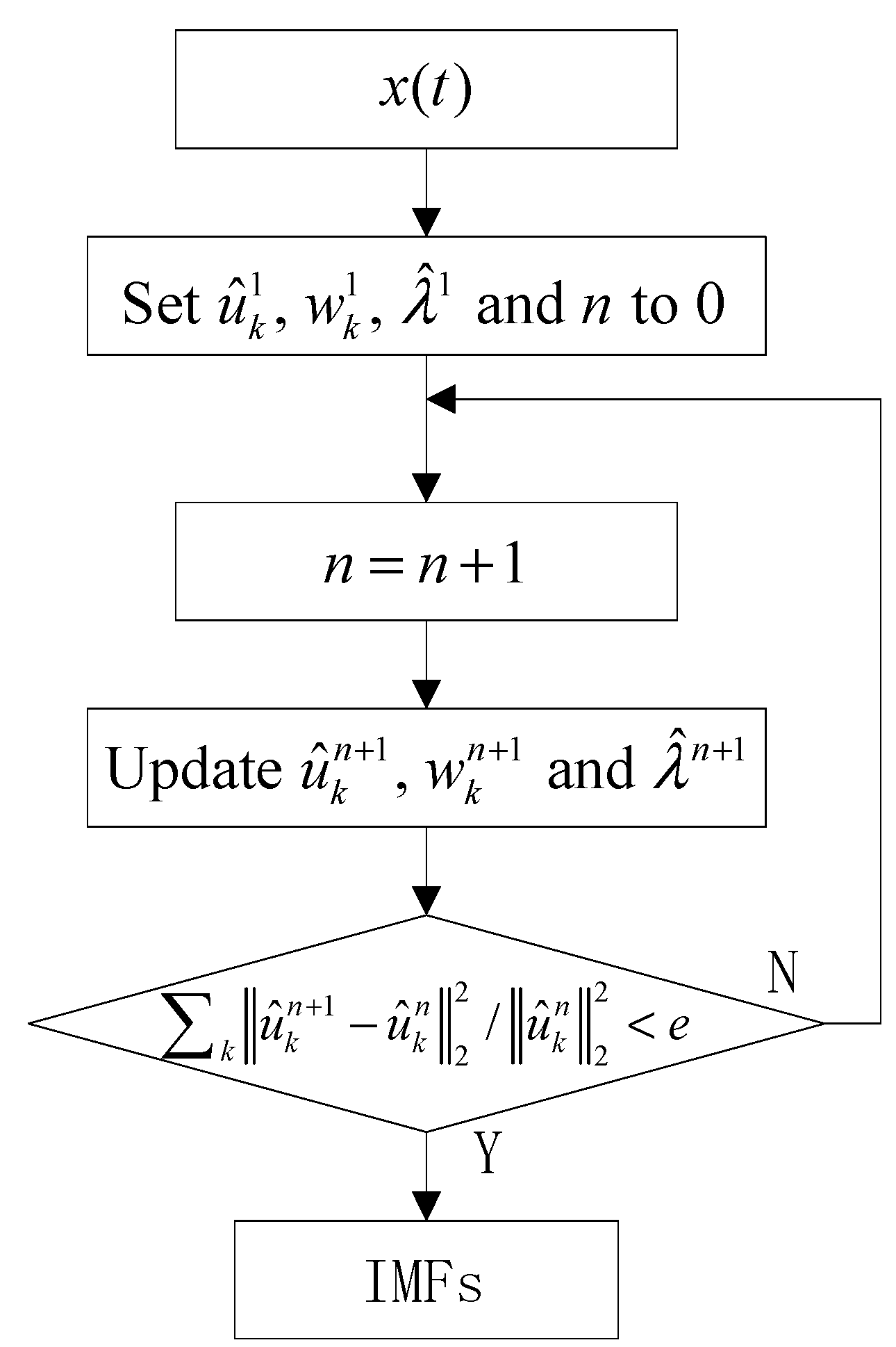
2.1. VMD
2.2. DCO
- (1)
- Put periodic signal and noise signal into the system, DCO equation can be expressed in Equation (7).
- (2)
- Set , and to 0.5, 0 and 0. The Runge-Kutta of the fourth order is used for a solution of DCO equation.
- (3)
- We can determine whether the angular frequency of the periodic signal is close to according to the system state. When the system state is the great periodic state, this means that the angular frequency of the periodic signal is approximated as , and vice versa. More detailed explanations about DCO can be found elsewhere [27,28].
2.3. KPE
- (1)
- KPE, as an improved PE, is defined as the distance between the time series and white Gaussian noise. Therefore, KPE and PE have a totally opposite trend. For example, when the time series is white Gaussian noise, PE and KPE are close to 1 and 0 respectively.
- (2)
- The equations of KPE and PE are different. KPE and PE can be expressed aswhere and represent KPE and PE, and are the number of reconstructed vectors and the embedded dimension, represents -th probability of symbol sequence.
- (3)
- Compared with PE, KPE has better robustness for time series of different lengths.
3. Frequency Feature Extraction Method for Underwater Acoustic Signal
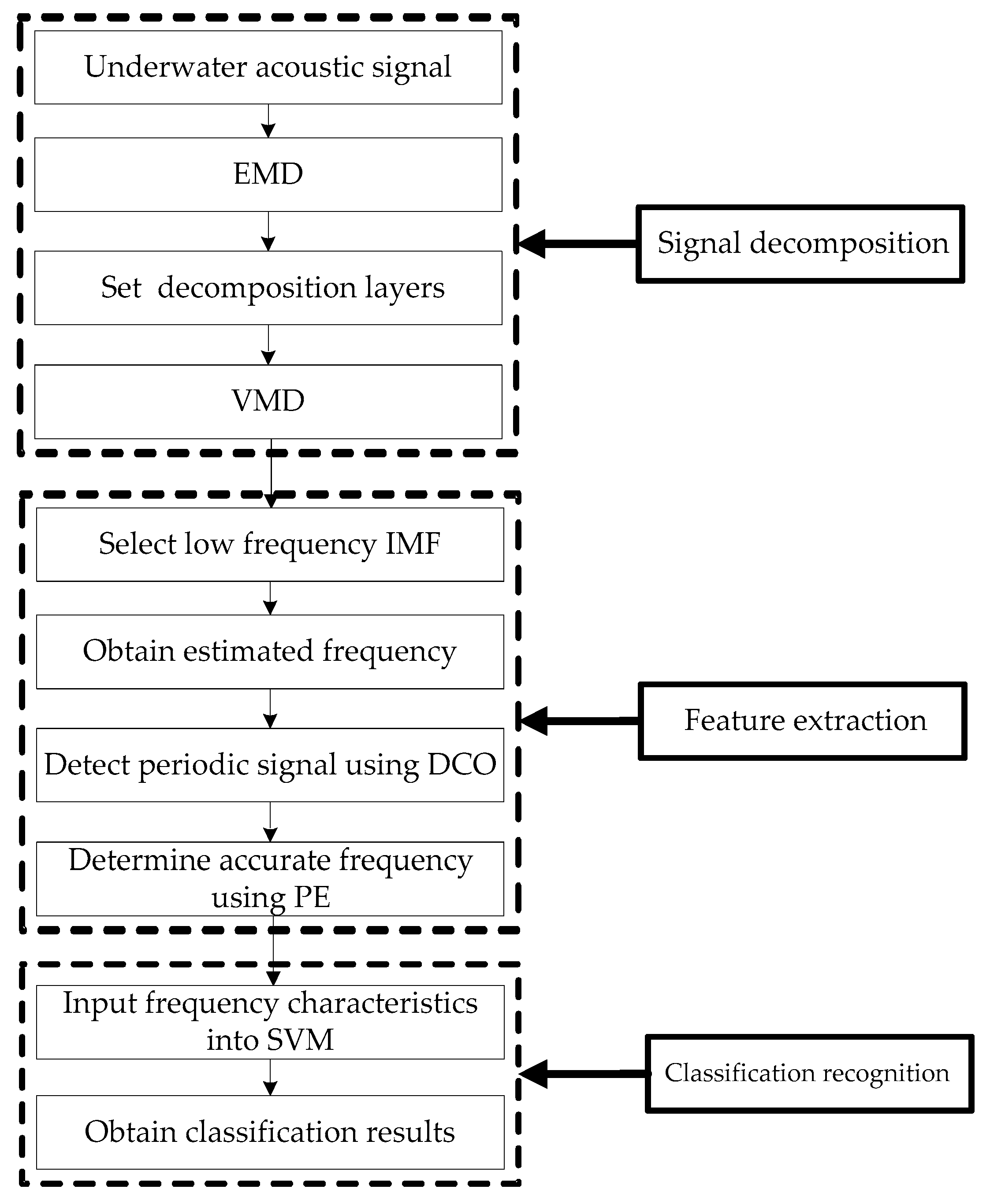
- Step 1:
- Signal decomposition.
- (1)
- Collect underwater acoustic signals by sensors;
- (2)
- Decompose underwater acoustic signals by EMD, M IMFs can be obtained;
- (3)
- Set the decomposition layers of VMD to M;
- (4)
- Decompose underwater acoustic signals by VMD.
- Step 2:
- Feature extraction.
- (1)
- Select the low-frequency IMF for the research, such as the last IMF;
- (2)
- Obtain estimated frequency of selected IMF by VMD;
- (3)
- Detect periodic signal of selected IMF using DCO;
- (4)
- When the phase track of selected IMF is in great periodic, and the KPE of DCO system output reaches the maximum, we can determine the accurate frequency of selected IMF.
- Step 3:
- Classification recognition.
- (1)
- Input frequency characteristics of different kinds of underwater acoustic signals into SVM;
- (2)
- Obtain classification results of different kinds of underwater acoustic signals.
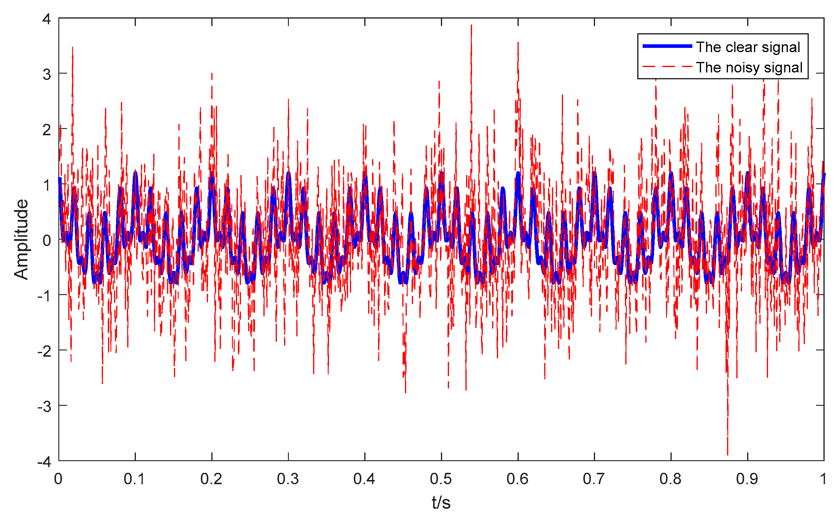
4. Frequency Feature Extraction for Simulation Signal
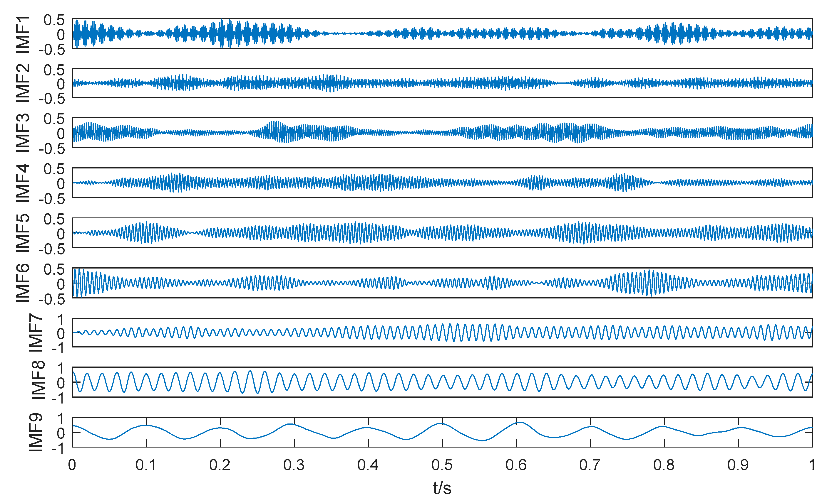
4.1. VMD of Simulation Signal
4.2. Frequency Feature Extraction of IMF Using DCO and KPE
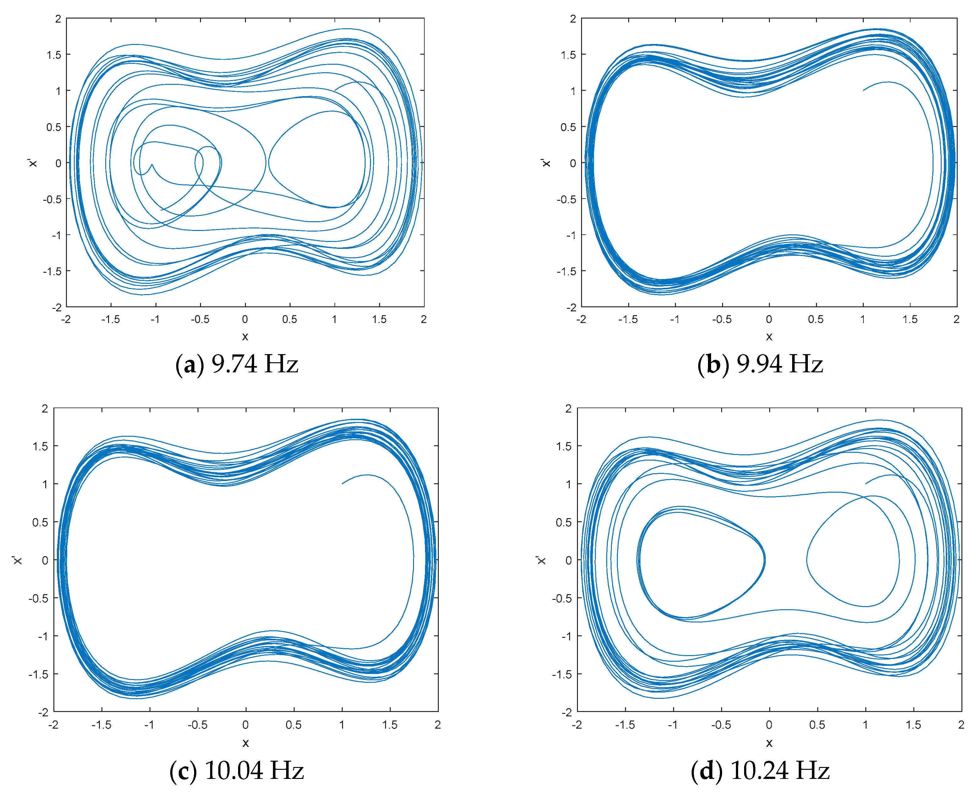
4.2.1. Frequency Feature Extraction of IMF9
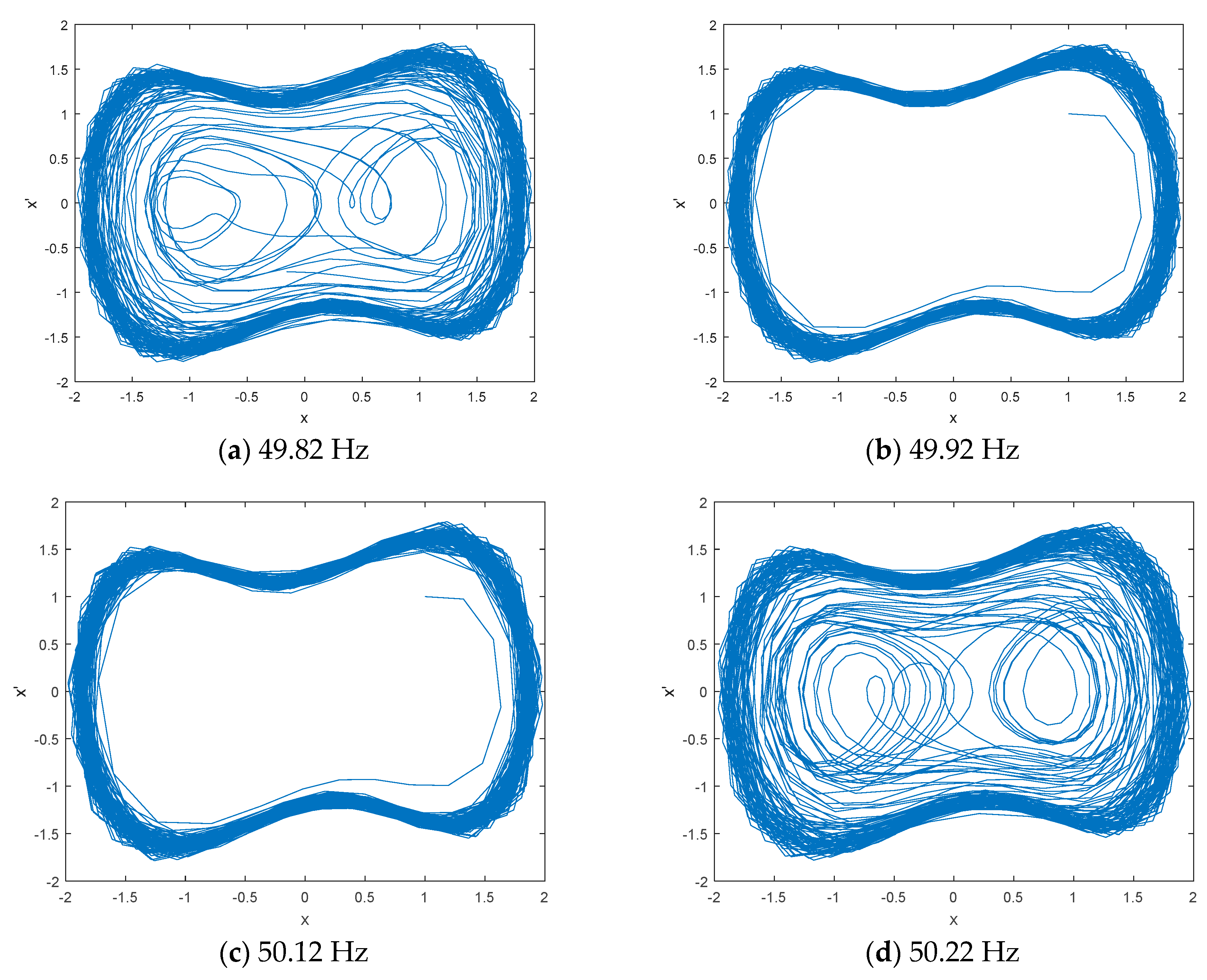
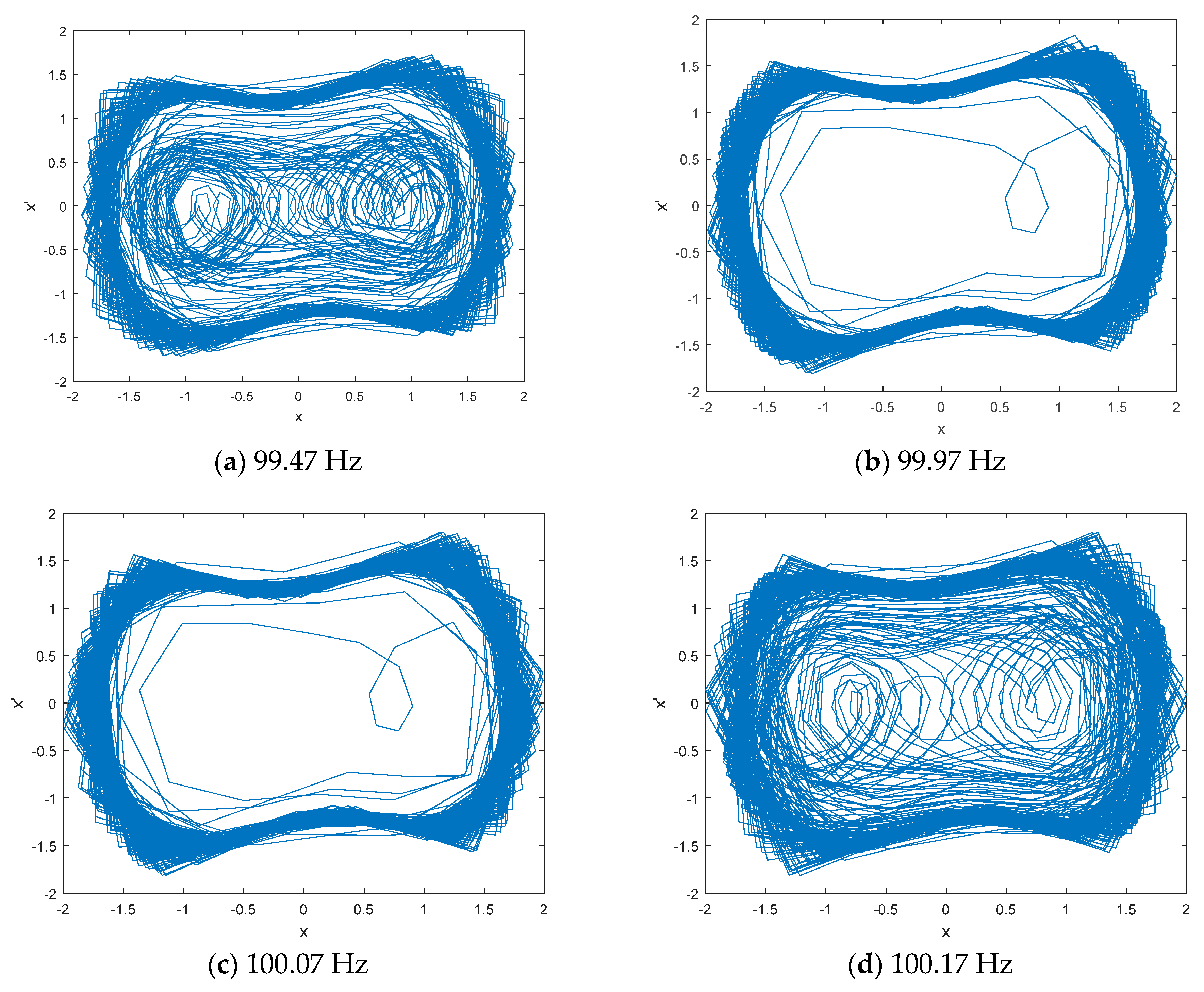
4.2.2. Frequency Feature Extraction of IMF8 and IMF7
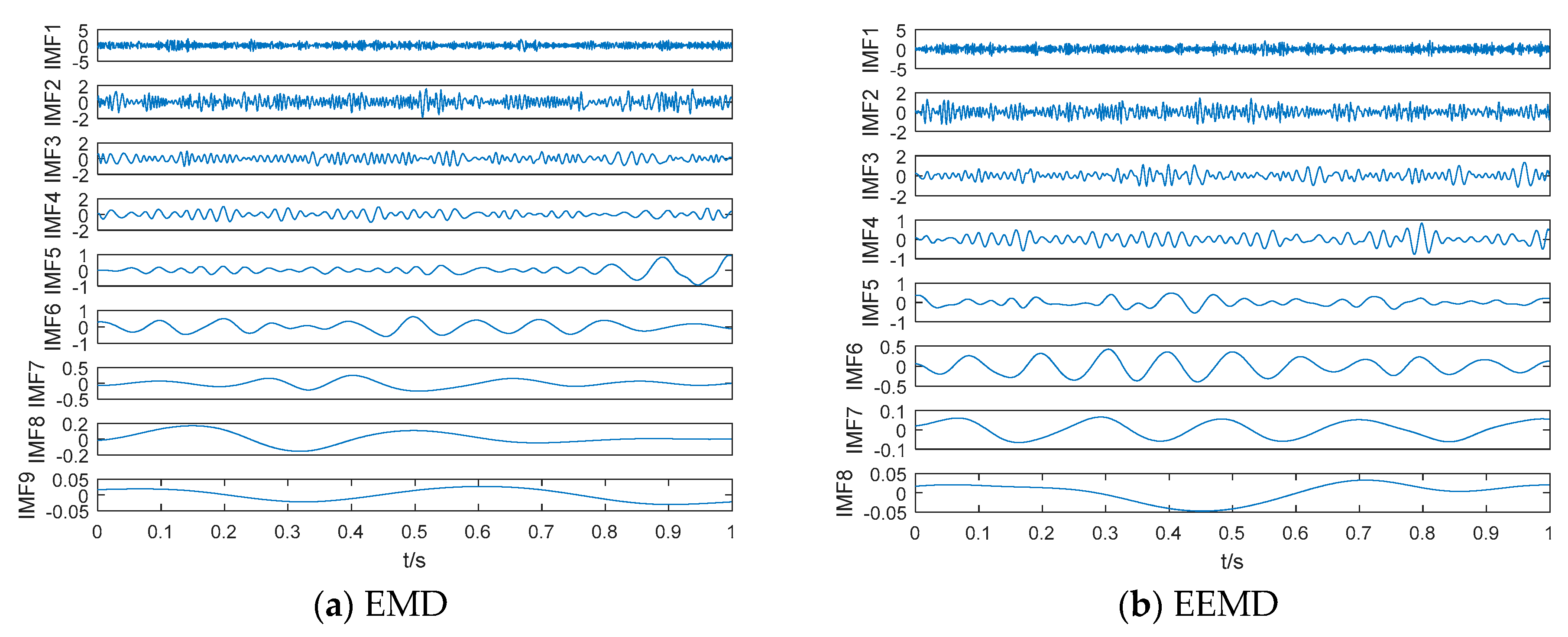
4.3. Comparison of Different Frequency Feature Extraction Methods
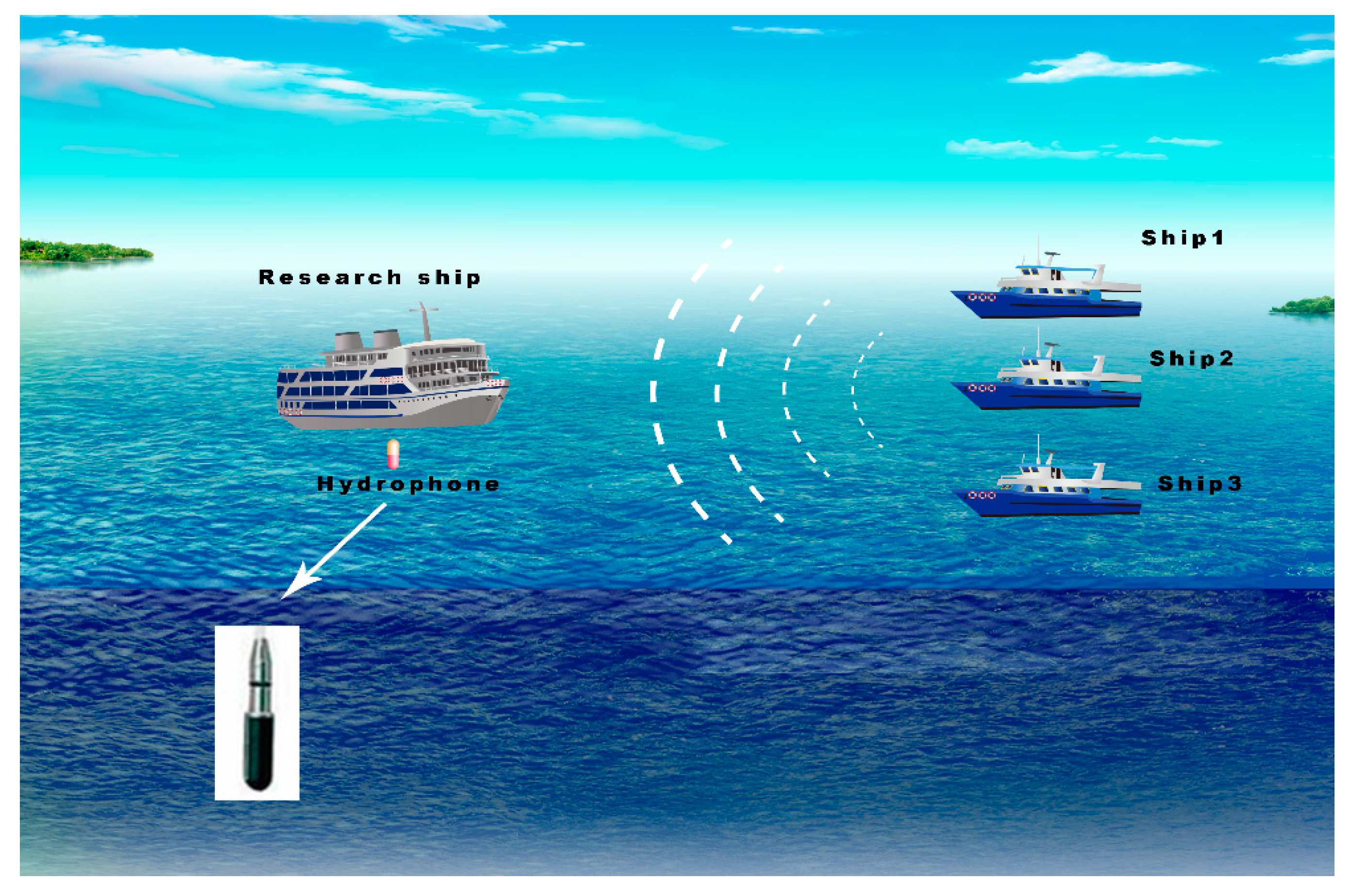
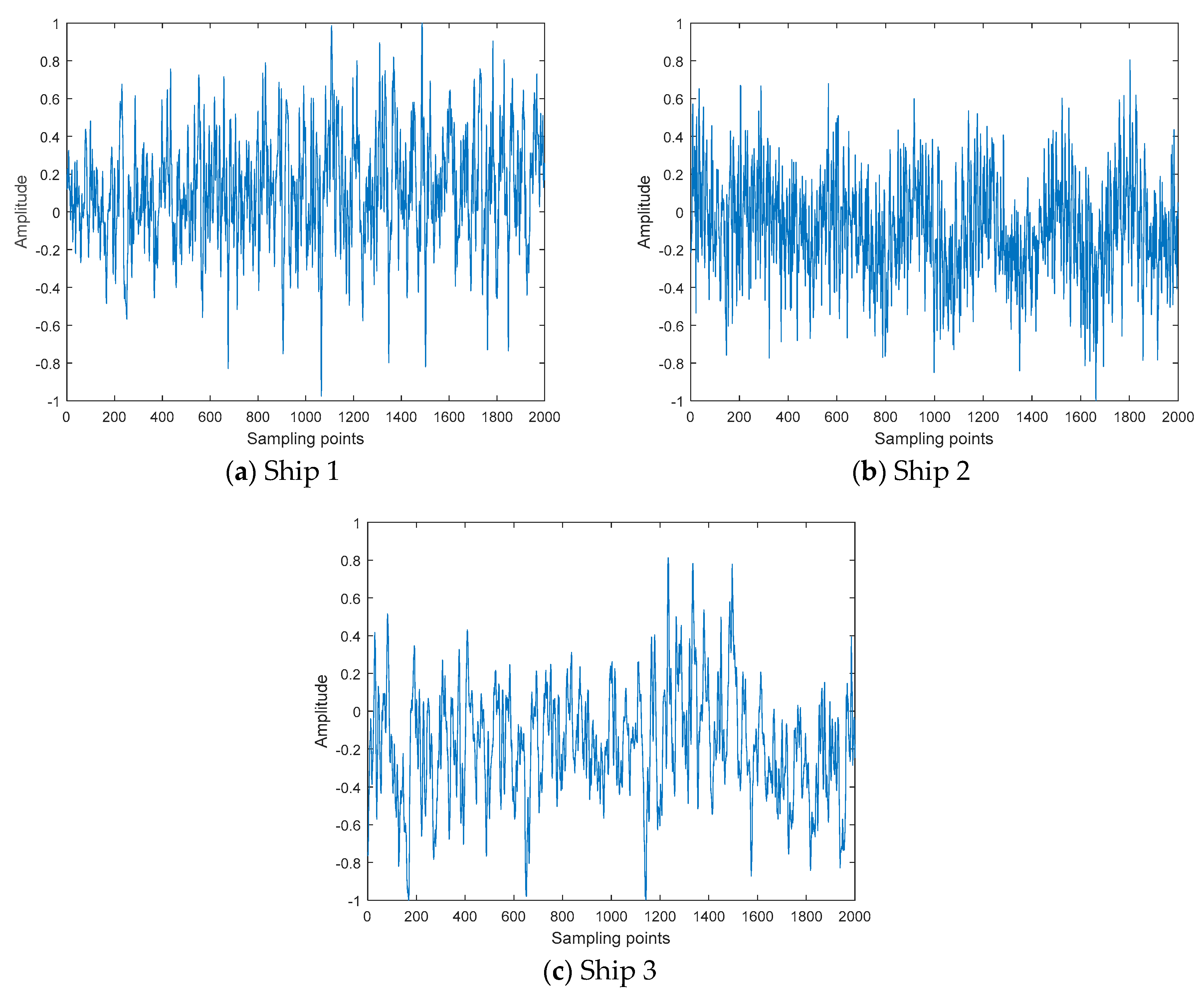
5. Application in Underwater Acoustic Signals
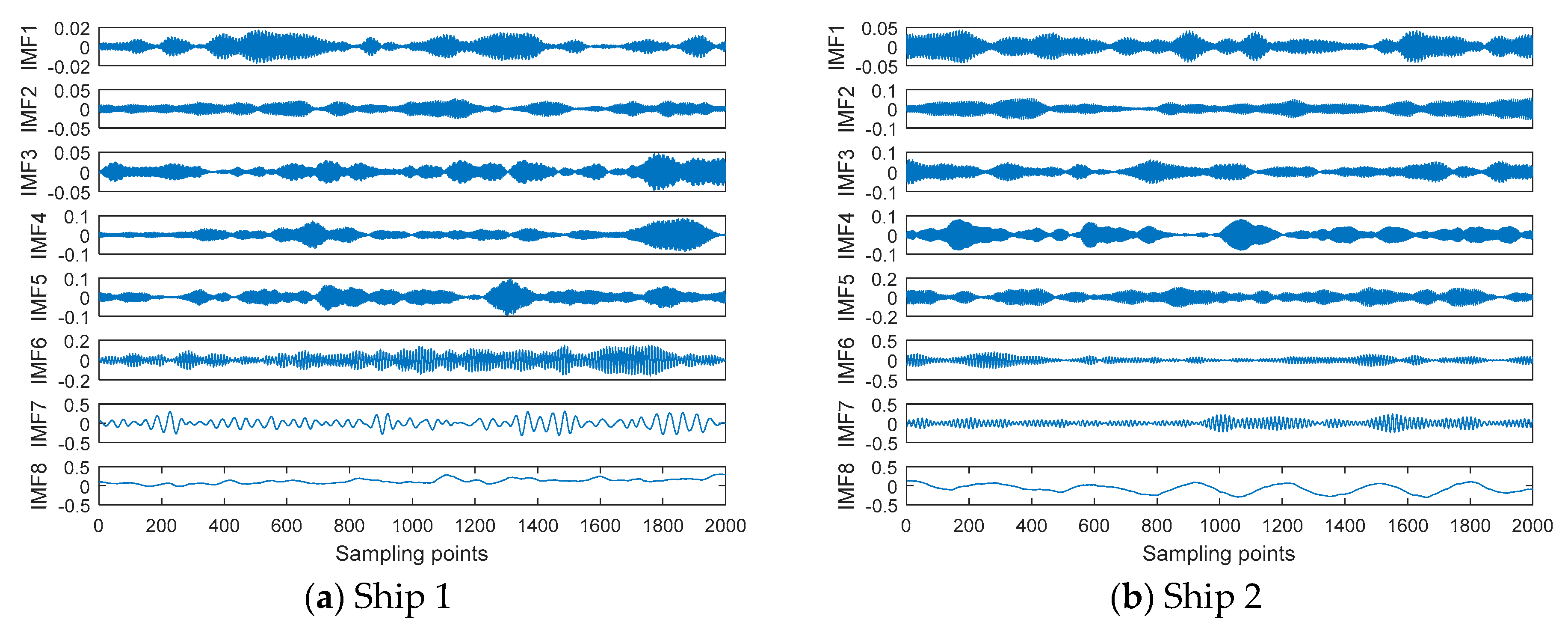
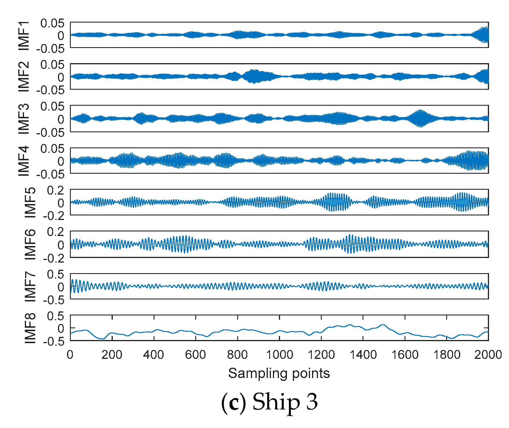
5.1. VMD of Ship-Radiated Noise Signal
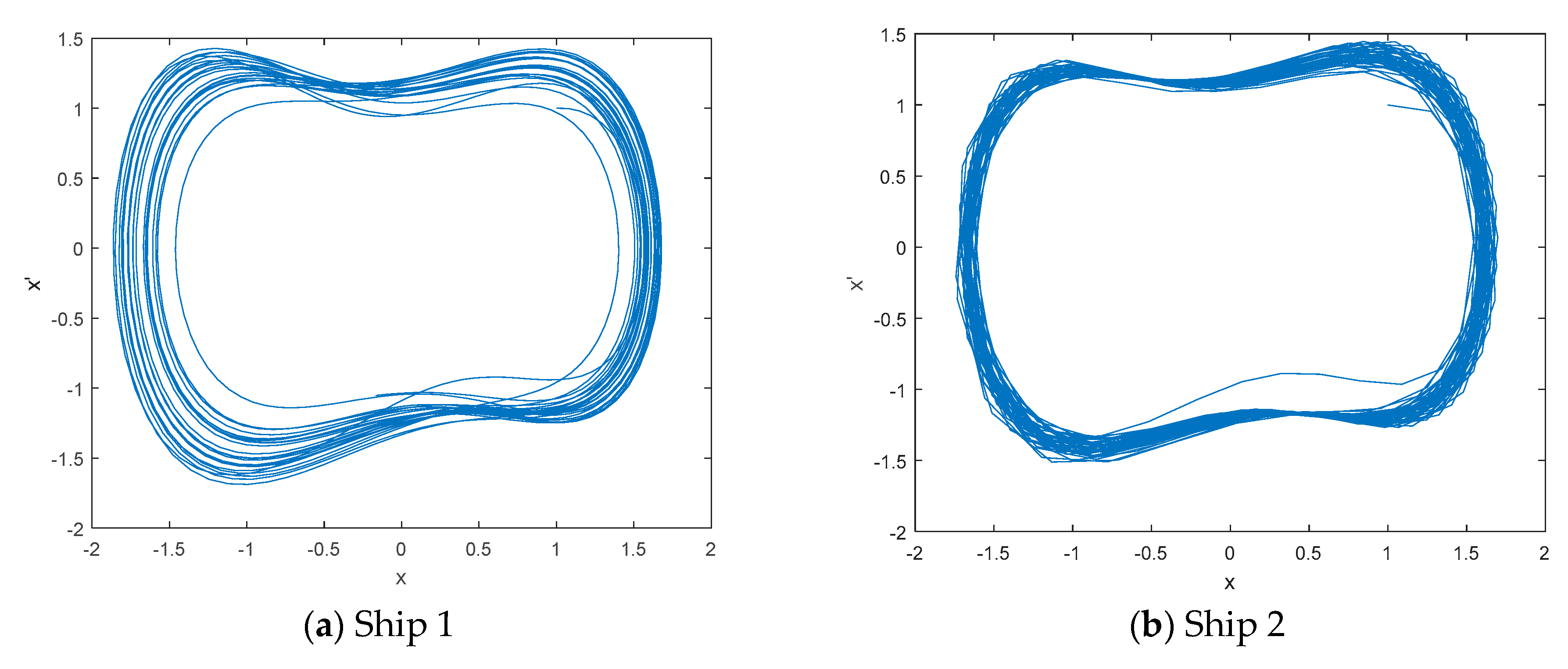
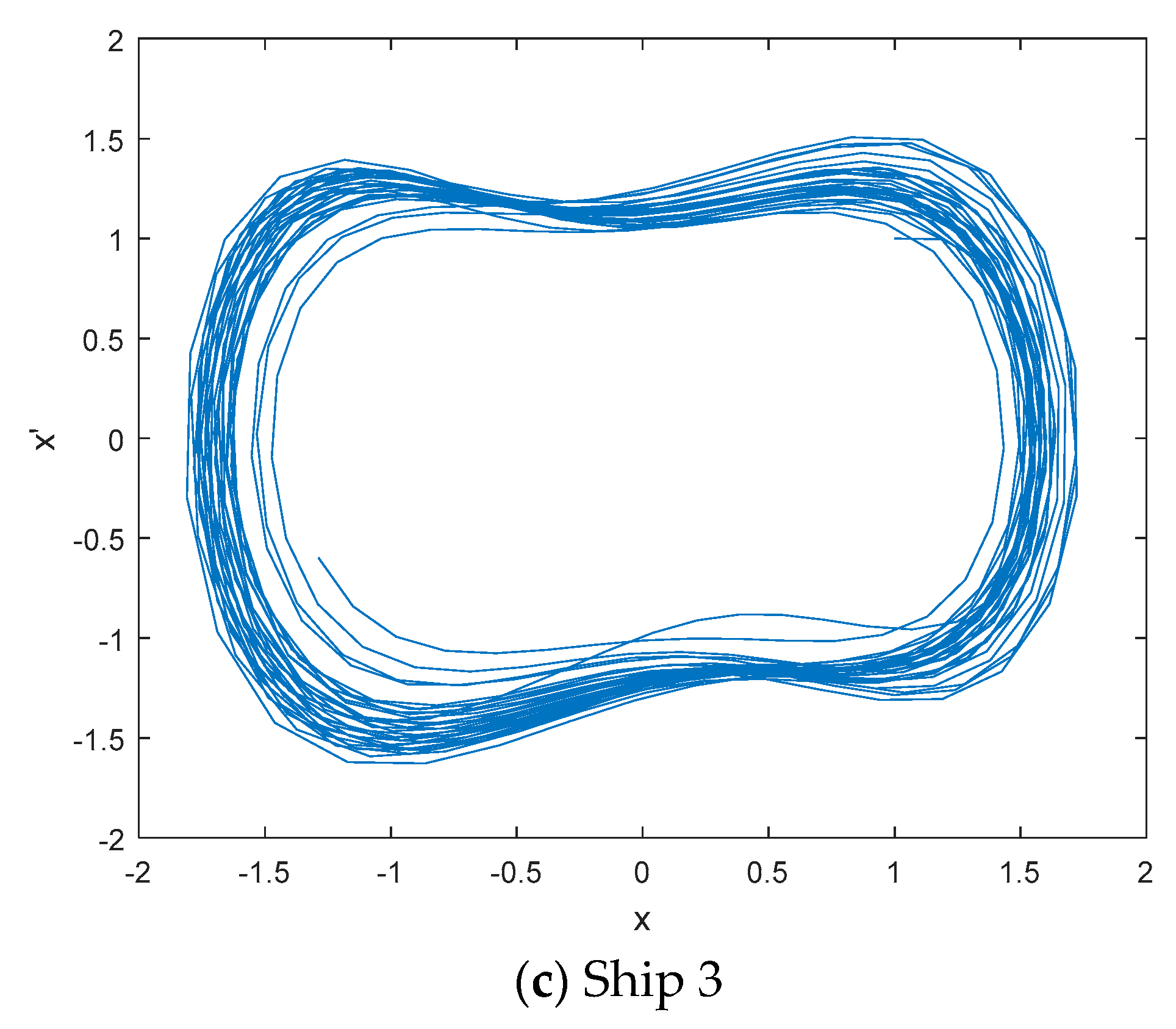
5.2. Frequency Feature Extraction of Line Spectrum
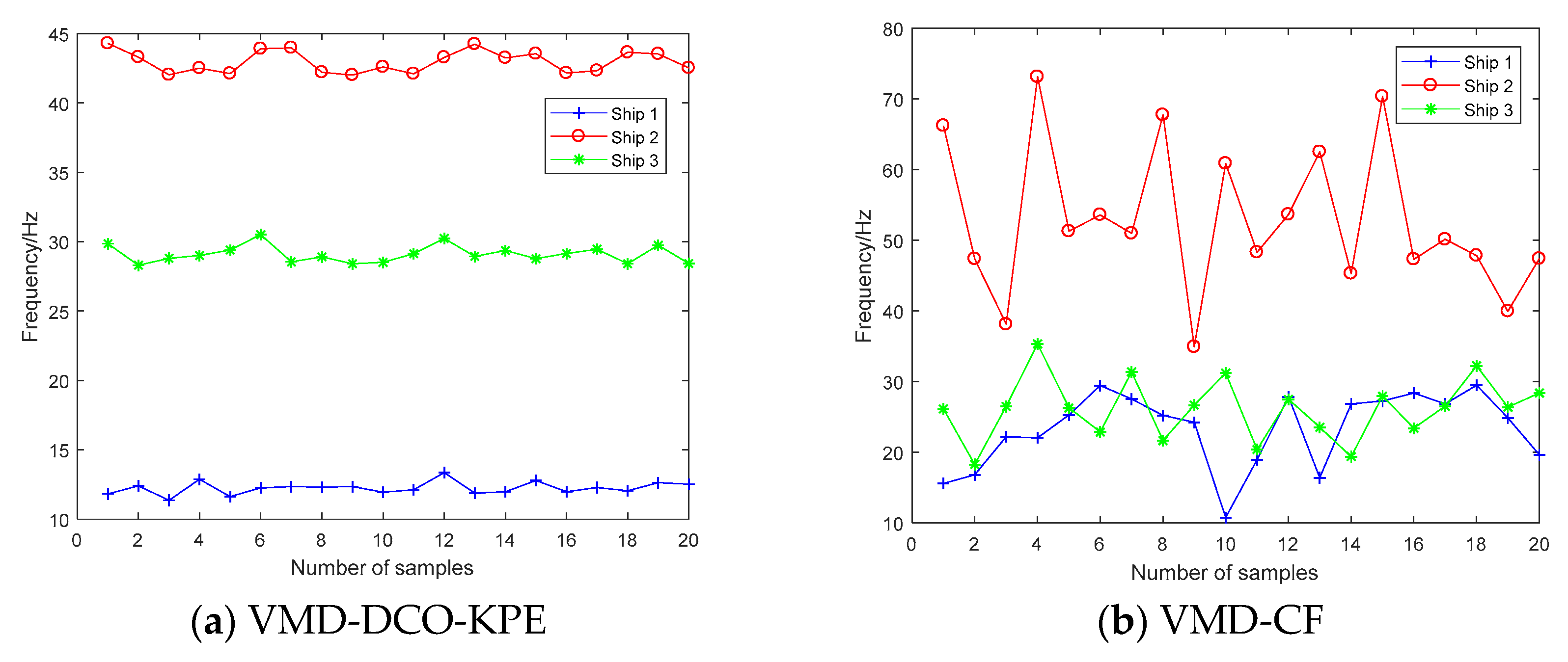
5.3. Comparison of Different Frequency Feature Extraction Methods
6. Conclusions
- (1)
- DCO is first used to detect the frequency of IMF by VMD for underwater acoustic signals in this paper.
- (2)
- KPE is first used to determine the frequency of IMF combined with DCO for underwater acoustic signals in this paper.
- (3)
- VMD-DCO-PE is successfully applied to extract the frequency feature of a simulation signal. Compared with EMD-CF, EEMD-CF and VMD-CF, VMD-DCO-KPE can be more accurate and efficient to extract the frequency feature of a simulation signal.
- (4)
- VMD-DCO-KPE is also applied to extract the frequency feature extraction of line spectrum for underwater acoustic signal. VMD-DCO-KPE has better classification performance than EMD-CF, EEMD-CF and VMD-CF.
Author Contributions
Funding
Conflicts of Interest
References
- Urick, R.J. Principles of Underwater Sound, 3rd ed.; McGraw-Hill: New York, NY, USA, 1983. [Google Scholar]
- Li, Y.; Li, Y.; Chen, X.; Yu, J. A Novel Feature Extraction Method for Ship-Radiated Noise Based on Variational Mode Decomposition and Multi-Scale Permutation Entropy. Entropy 2017, 19, 342. [Google Scholar] [CrossRef]
- Li, Y.; Li, Y.; Chen, X.; Yu, J. Research on Ship-Radiated Noise Denoising Using Secondary Variational Mode Decomposition and Correlation Coefficient. Sensors 2018, 18, 48. [Google Scholar] [CrossRef]
- Villecco, F. On the Evaluation of Errors in the Virtual Design of Mechanical Systems. Machines 2018, 6, 36. [Google Scholar] [CrossRef]
- Wang, S.; Zeng, X. Robust underwater noise targets classification using auditory inspired time-frequencyanalysis. Appl. Acoust. 2014, 78, 68–76. [Google Scholar] [CrossRef]
- Xu, L.; Yang, K.; Yang, Q. Joint time-frequency inversion for seabed properties of ship noise on a vertical line array in South China Sea. IEEE Access 2018, 6, 62856–62864. [Google Scholar] [CrossRef]
- Gassmann, M.; Wiggins, S.M.; Hildebrand, J.A. Deep-water measurements of container ship radiated noise signatures and directionality. J. Acoust. Soc. Am. 2017, 142, 1563. [Google Scholar] [CrossRef] [PubMed]
- Wang, Y.H.; Hu, K.; Lo, M.T. Uniform phase empirical mode decomposition: An optimal hybridization of masking signal and ensemble approaches. IEEE Access 2018, 6, 34819–34833. [Google Scholar] [CrossRef]
- Wang, J.L.; Wei, Q.X.; Zhao, L.Q.; Yu, T.; Han, R. An improved empirical mode decomposition method using second generation wavelets interpolation. Digit. Signal Process. 2018, 79, 164–174. [Google Scholar] [CrossRef]
- Chen, T.; Ju, S.; Yuan, X.; Elhoseny, M.; Ren, F.; Fan, M.; Chen, Z. Emotion recognition using empirical mode decomposition and approximation entropy. Comput. Electr. Eng. 2018, 72, 383–392. [Google Scholar] [CrossRef]
- Zhang, X.; Liang, Y.; Zhou, J.; Zhou, J.; Zang, Y. A novel bearing fault diagnosis model integrated permutation entropy, ensemble empirical mode decomposition and optimized SVM. Measurement 2015, 69, 164–179. [Google Scholar] [CrossRef]
- Chu, H.; Wei, J.; Qiu, J. Monthly Streamflow Forecasting Using EEMD-Lasso-DBN Method Based on Multi-Scale Predictors Selection. Water 2018, 10, 1486. [Google Scholar] [CrossRef]
- Huang, Y.; Liu, S.; Yang, L. Wind Speed Forecasting Method Using EEMD and the Combination Forecasting Method Based on GPR and LSTM. Sustainability 2018, 10, 3693. [Google Scholar] [CrossRef]
- Singh, J.; Darpe, A.K.; Singh, S.P. Bearing damage assessment using Jensen-Rényi Divergence based on EEMD. Mech. Syst. Signal Process. 2017, 87, 307–339. [Google Scholar] [CrossRef]
- Yeh, J.R.; Shieh, J.S.; Huang, N.E. Complementary ensemble empirical mode decomposition: A novel noise enhanced data analysis method. Adv. Adapt. Data Anal. 2010, 2, 135–156. [Google Scholar] [CrossRef]
- Liu, H.; Mi, X.W.; Li, Y.F. Comparison of two new intelligent wind speed forecasting approaches based on Wavelet packet decomposition, complete ensemble empirical mode decomposition with adaptive noise and artificial neural networks. Energ. Conv. Manag. 2018, 155, 188. [Google Scholar] [CrossRef]
- Lv, Y.; Yuan, R.; Wang, T.; Li, H.; Song, G. Health Degradation Monitoring and Early Fault Diagnosis of a Rolling Bearing Based on CEEMDAN and Improved MMSE. Materials 2018, 11, 1009. [Google Scholar] [CrossRef]
- Dai, S.; Niu, D.; Li, Y. Daily Peak Load Forecasting Based on Complete Ensemble Empirical Mode Decomposition with Adaptive Noise and Support Vector Machine Optimized by Modified Grey Wolf Optimization Algorithm. Energies 2018, 11, 163. [Google Scholar] [CrossRef]
- Bin Queyam, A.; Kumar Pahuja, S.; Singh, D. Quantification of Feto-Maternal Heart Rate from Abdominal ECG Signal Using Empirical Mode Decomposition for Heart Rate Variability Analysis. Technologies 2017, 5, 68. [Google Scholar] [CrossRef]
- Dragomiretskiy, K.; Zosso, D. Variational mode decomposition. IEEE Trans. Signal Process. 2014, 62, 531–544. [Google Scholar] [CrossRef]
- Li, Y.; Li, Y.; Chen, X.; Yu, J. Denoising and Feature Extraction Algorithms Using NPE Combined with VMD and Their Applications in Ship-Radiated Noise. Symmetry 2017, 9, 256. [Google Scholar] [CrossRef]
- Cai, W.; Yang, Z.; Wang, Z.; Wang, Y. A New Compound Fault Feature Extraction Method Based on Multipoint Kurtosis and Variational Mode Decomposition. Entropy 2018, 20, 521. [Google Scholar] [CrossRef]
- Wan, S.; Chen, L.; Dou, L.; Zhou, J. Mechanical Fault Diagnosis of HVCBs Based on Multi-Feature Entropy Fusion and Hybrid Classifier. Entropy 2018, 20, 847. [Google Scholar] [CrossRef]
- Tripathy, R.K.; Paternina, M.R.A.; Arrieta, J.G.; Pattanaik, P. Automateddetection of atrialfibrillation ECG signalsusing twostage VMD and atrialfibrillation diagnosis index. J. Mech. Med. Biol. 2017, 17, 840–844. [Google Scholar] [CrossRef]
- Wang, G.; Chen, D.; Lin, J.; Chen, X. The application of chaotic oscillators to weak signal detection. IEEE Trans. Ind. Electron. 1999, 46, 440–444. [Google Scholar] [CrossRef]
- Li, Y.; Shi, Y.; Ma, H.; Yang, B. Chaotic detection method for weak square wave signal submerged in colored noise. Chin. J. Electron. 2004, 32, 87–90. [Google Scholar]
- Lai, Z.; Leng, Y.; Sun, J.; Fan, B. Weak characteristic signal detection based on scale transformation of Duffing oscillator. Acta Phys. Sin. 2012, 61, 050503. [Google Scholar]
- Chen, Z.; Li, Y.; Chen, X. Underwater acoustic weak signal detection based on Hilbert transform and intermittent chaos. Acta Phys. Sin. 2015, 64, 200502. [Google Scholar]
- Bandt, C.; Pompe, B. Permutation entropy: A natural complexity measure for time series. Phys. Rev. Lett. 2002, 88, 174102. [Google Scholar] [CrossRef]
- Zhang, J.; Hou, G.; Cao, K.; Ma, B. Operation conditions monitoring of flood discharge structure based on variance dedication rate and permutation entropy. Nonlinear Dyn. 2018, 93, 1–15. [Google Scholar] [CrossRef]
- Bandt, C. A new kind of permutation entropy used to classify sleep stages from invisible EEG microstructure. Entropy 2017, 19, 197. [Google Scholar] [CrossRef]
- Haruna, T. Partially ordered permutation complexity of coupled time series. Phys. D Nonlinear Phenom. 2018, 388, 40–44. [Google Scholar] [CrossRef]
- Hu, Q.; Hao, B.; Lv, L. Feature extraction model for underwater target radiated noise. Torpedo Technol. 2008, 16, 38. [Google Scholar]
- Liu, S.; Zhang, X.; Niu, Y. Feature extraction and classification experiment of underwater acoustic signals based on energy spectrum of IMF’s. Comput. Eng. Appl. 2014, 50, 203–206. [Google Scholar]
- Yang, H.; Li, Y.; Li, G. Energy analysis of ship-radiated noise based on ensemble empirical mode decomposition. J. Vib. Shock 2015, 34, 55–59. [Google Scholar]

| IMF1 | IMF2 | IMF3 | IMF4 | IMF5 | IMF6 | IMF7 | IMF8 | IMF9 |
|---|---|---|---|---|---|---|---|---|
| 442.23 Hz | 392.59 Hz | 321.89 Hz | 264.65 Hz | 227.73 Hz | 168.37 Hz | 99.47 Hz | 50.12 Hz | 10.14 Hz |
| 9.95 Hz | 9.96 Hz | 9.97 Hz | 9.98 Hz | 9.99 Hz | 10.00 Hz | 10.01 Hz |
|---|---|---|---|---|---|---|
| 0.313618 | 0.313618 | 0.313622 | 0.313630 | 0.313622 | 0.313618 | 0.313616 |
| 49.96 Hz | 49.97 Hz | 49.98 Hz | 49.99 Hz | 50.00 Hz | 50.01 Hz | 50.02 Hz |
|---|---|---|---|---|---|---|
| 0.240762 | 0.240779 | 0.240813 | 0.240961 | 0.240884 | 0.240761 | 0.240753 |
| 100.00 Hz | 100.01 Hz | 100.02 Hz | 100.03 Hz | 100.04 Hz | 100.05 Hz | 100.06 Hz |
|---|---|---|---|---|---|---|
| 0.163238 | 0.163396 | 0.164079 | 0.164159 | 0.164076 | 0.164027 | 0.163390 |
| IMF1 | IMF2 | IMF3 | IMF4 | IMF5 | IMF6 | IMF7 | IMF8 | IMF9 |
|---|---|---|---|---|---|---|---|---|
| 319.2 Hz | 147.13 Hz | 68.94 Hz | 43.66 Hz | 19.54 Hz | 9.68 Hz | 6.32 Hz | 3.02 Hz | 1.97 Hz |
| IMF1 | IMF2 | IMF3 | IMF4 | IMF5 | IMF6 | IMF7 | IMF8 |
|---|---|---|---|---|---|---|---|
| 338.07 Hz | 149.78 Hz | 73.74 Hz | 44.07 Hz | 16.26 Hz | 9.72 Hz | 4.41 Hz | 2.37 Hz |
| Methods | 10 Hz | 50 Hz | 100 Hz |
|---|---|---|---|
| EMD-CF | 9.68 Hz | 43.66 Hz | 68.94 Hz |
| EEMD-CF | 9.72 Hz | 44.07 Hz | 73.74 Hz |
| VMD-CF | 10.14 Hz | 50.12 Hz | 99.47 Hz |
| VMD-DCO-KPE | 9.98 Hz | 49.99 Hz | 100.03 Hz |
| Ship 1 | Ship 2 | Ship 3 |
|---|---|---|
| 15.59 Hz | 66.18 Hz | 26.11 Hz |
| Ship 1 | Ship 2 | Ship 3 |
|---|---|---|
| 11.82 Hz | 44.29 Hz | 29.85 Hz |
| EMD-CF | EEMD-CF | VMD-CF | VMD-DCO-KPE |
|---|---|---|---|
| 67.33% | 74.67% | 80.67% | 100% |
© 2019 by the authors. Licensee MDPI, Basel, Switzerland. This article is an open access article distributed under the terms and conditions of the Creative Commons Attribution (CC BY) license (http://creativecommons.org/licenses/by/4.0/).
Share and Cite
Li, Y.; Chen, X.; Yu, J.; Yang, X. A Fusion Frequency Feature Extraction Method for Underwater Acoustic Signal Based on Variational Mode Decomposition, Duffing Chaotic Oscillator and a Kind of Permutation Entropy. Electronics 2019, 8, 61. https://doi.org/10.3390/electronics8010061
Li Y, Chen X, Yu J, Yang X. A Fusion Frequency Feature Extraction Method for Underwater Acoustic Signal Based on Variational Mode Decomposition, Duffing Chaotic Oscillator and a Kind of Permutation Entropy. Electronics. 2019; 8(1):61. https://doi.org/10.3390/electronics8010061
Chicago/Turabian StyleLi, Yuxing, Xiao Chen, Jing Yu, and Xiaohui Yang. 2019. "A Fusion Frequency Feature Extraction Method for Underwater Acoustic Signal Based on Variational Mode Decomposition, Duffing Chaotic Oscillator and a Kind of Permutation Entropy" Electronics 8, no. 1: 61. https://doi.org/10.3390/electronics8010061
APA StyleLi, Y., Chen, X., Yu, J., & Yang, X. (2019). A Fusion Frequency Feature Extraction Method for Underwater Acoustic Signal Based on Variational Mode Decomposition, Duffing Chaotic Oscillator and a Kind of Permutation Entropy. Electronics, 8(1), 61. https://doi.org/10.3390/electronics8010061