Filtering Methods for Efficient Dynamic Access Control in 5G Massive Machine-Type Communication Scenarios

Abstract

One of the three main use cases of the fifth generation of mobile networks (5G) is massive machine-type communications (mMTC). The latter refers to the highly synchronized accesses to the cellular base stations from a great number of wireless devices, as a product of the automated exchange of small amounts of data. Clearly, an efficient mMTC is required to support the Internet-of-Things (IoT). Nevertheless, the method to change from idle to connected mode, known as the random access procedure (RAP), of 4G has been directly inherited by 5G, at least, until the first phase of standardization. Research has demonstrated the RAP is inefficient to support mMTC, hence, access control schemes are needed to obtain an adequate performance. In this paper, we compare the benefits of using different filtering methods to configure an access control scheme included in the 5G standards: the access class barring (ACB), according to the intensity of access requests. These filtering methods are a key component of our proposed ACB configuration scheme, which can lead to more than a three-fold increase in the probability of successfully completing the random access procedure under the most typical network configuration and mMTC scenario.

1. Introduction

The first phase of standardization for the future 5th generation of mobile networks (5G) was concluded in the Release 15 of the 3GPP Evolved Universal Terrestrial Radio Access (E-UTRA) specifications [1]. Previous mobile generations, 3G and 4G, have merely focused on providing a faster and better mobile broadband service. Instead, 5G relies on three main use cases: massive machine-type communication (mMTC), enhanced mobile broadband (eMBB), and ultra-reliable low-latency communication (URLLC). The support for mMTC and URLLC are the main distinctive characteristics of 5G, and are expected to enable a great number of novel applications. These include, among others, the Internet-of-Things (IoT), where every daily-life object is connected to the Internet to empower a wide range of functionalities.

Nevertheless, the Release 15 of the 3GPP specifications introduced few advances in terms of mMTC support when compared to Release 14. One of the most critical requirements to efficiently support mMTC in 5G was to introduce enhancements to the random access procedure (RAP) of 4G. The RAP is the method used by user equipments (UEs) to switch from idle to connected mode. In other words, it is the method used by UEs for initial access to the cellular network.

Several studies have demonstrated the inefficacy of the RAP, as defined by the 3GPP [1], to support mMTC in 4G [2,3,4,5]. Specifically, severe congestion can occur when a bulk of UE access attempts occur in a highly synchronized manner. The latter, which is a typical behavior in mMTC applications, is likely to exceed the signaling capacity of the cellular system. Since the RAP remains the same in 5G, the same limitations and problems persist.

Enhancements are expected to be introduced to the RAP in the following standardization phases of 5G. At the present time, it remains uncertain whether these will be sufficient to support mMTC applications efficiently. On the other hand, access control schemes present an appealing solution to congestion. Because of this, a wide range of access control schemes have been proposed in the literature [6,7,8,9,10,11].

One of the most promising access control schemes is the access class barring (ACB); hence, it has been included in the LTE-A Radio Resource Control (RRC) specifications [1]. The ACB scheme redistributes the UE access attempts through time. For this, each UE may delay the beginning of its RAP according to the barring parameters: barring rate and mean barring time. If the barring parameters are correctly configured, sporadic periods of congestion can be relieved in exchange for a longer access delay. This is true even if barring parameters are selected beforehand and remain fixed throughout the congestion period [5,10,12,13]. However, congestion is a transitory phenomenon, so an adequate performance under several conditions can only be obtained by continuously adapting the barring parameters to the intensity of access attempts. Doing otherwise would increase the access delay of UEs during intervals in which no congestion occurs, but also fail to relieve congestion episodes that are more severe than expected. Needless to say, correctly configuring the barring parameters in real-time is a complicated task.

Numerous methods to continuously adapt the barring parameters have been proposed in the literature [9,14,15,16,17,18]; we refer to these methods simply as ACB configuration (ACBC) schemes. In other words, we use the term ACBC scheme to refer to any method or approach to select the barring parameters. In theory, some of the above-mentioned schemes can lead to a near-optimal performance in terms of success probability (i.e., probability of successfully completing the RAP) and access delay. However, most of these ACBC schemes were not designed for 3GPP cellular networks. Specifically, such a high performance is normally achieved by assuming an idealized ACB scheme and by setting extremely precise barring parameters, for which complex processes and bold assumptions are oftentimes needed. As a consequence, most of the ACBC schemes proposed in the literature cannot be implemented in the cellular systems [9,11,14,17].

Tello-Oquendo et al. presented one of the few ACBC schemes that were specifically designed for 3GPP cellular networks [18]. In particular, a reinforcement learning approach was utilized. However, results show that the performance achieved under the most typical mMTC scenario with the proposed ACBC scheme is lower than that of correctly selecting the fixed barring parameters beforehand.

In our previous work, we proposed an ACBC scheme that incorporates a filtering block [19]. In this block, the well-known least-mean square (LMS) algorithm was implemented. In particular, two different applications of the LMS were investigated: the adaptive line enhancer (ALE) and a novel twist on the latter, referred to as “pulling” ALE (PALE) [19]; preliminary work on the benefits of the PALE can be found in [8]. During previous work, we found our ACBC scheme is one of the few that can be implemented in 3GPP networks and that can provide a near-optimal performance, which greatly surpasses that of the ACB with fixed parameters, under different access request intensities [8,19].

The main motivation of the present study is to investigate the potential benefits of our ACBC scheme with different filtering methods, namely, the recursive least-squares (RLS) algorithm or fixed finite-duration impulse response (FIR) filters instead of the LMS. Each of these presents different characteristics in terms of the rate of convergence, numerical stability, and simplicity. Therefore, the main contributions of this paper are described in the following.

• Two different filtering methods are investigated, namely the RLS adaptive algorithm and a FIR filter. The benefits of these methods are compared to those of the LMS. The latter was the only algorithm considered in our previous work [8,19].
• An in-depth analysis of the tracking capabilities of the LMS and RLS adaptive algorithms in transient environments is presented.

We observed several filtering methods lead to an adequate operation of our ACBC scheme under the most typical mMTC scenario. However, the main difference between implementing an adaptive algorithm and a simple FIR filter is that, for the latter method, an additional mechanism is needed to reduce the access delay of UEs in mMTC scenarios that can be handled by the RAP itself. That is, when the intensity of access attempts is low when compared to the capacity of the RAP. Clearly, increasing the access delay of UEs in these cases is not beneficial. On the other hand, such a mechanism is not needed if some adaptive algorithm configurations are implemented.

The rest of the paper is organized as follows. The RAP and the ACB scheme are described in Section 2. Next, our ACBC scheme, the studied filtering methods, and the methodology used to assess the benefits of these methods are explained in Section 3. Our main results are presented in Section 4 and Section 5 concludes the paper.

2. Random Access Procedure (RAP) and Access Class Barring (ACB) Scheme

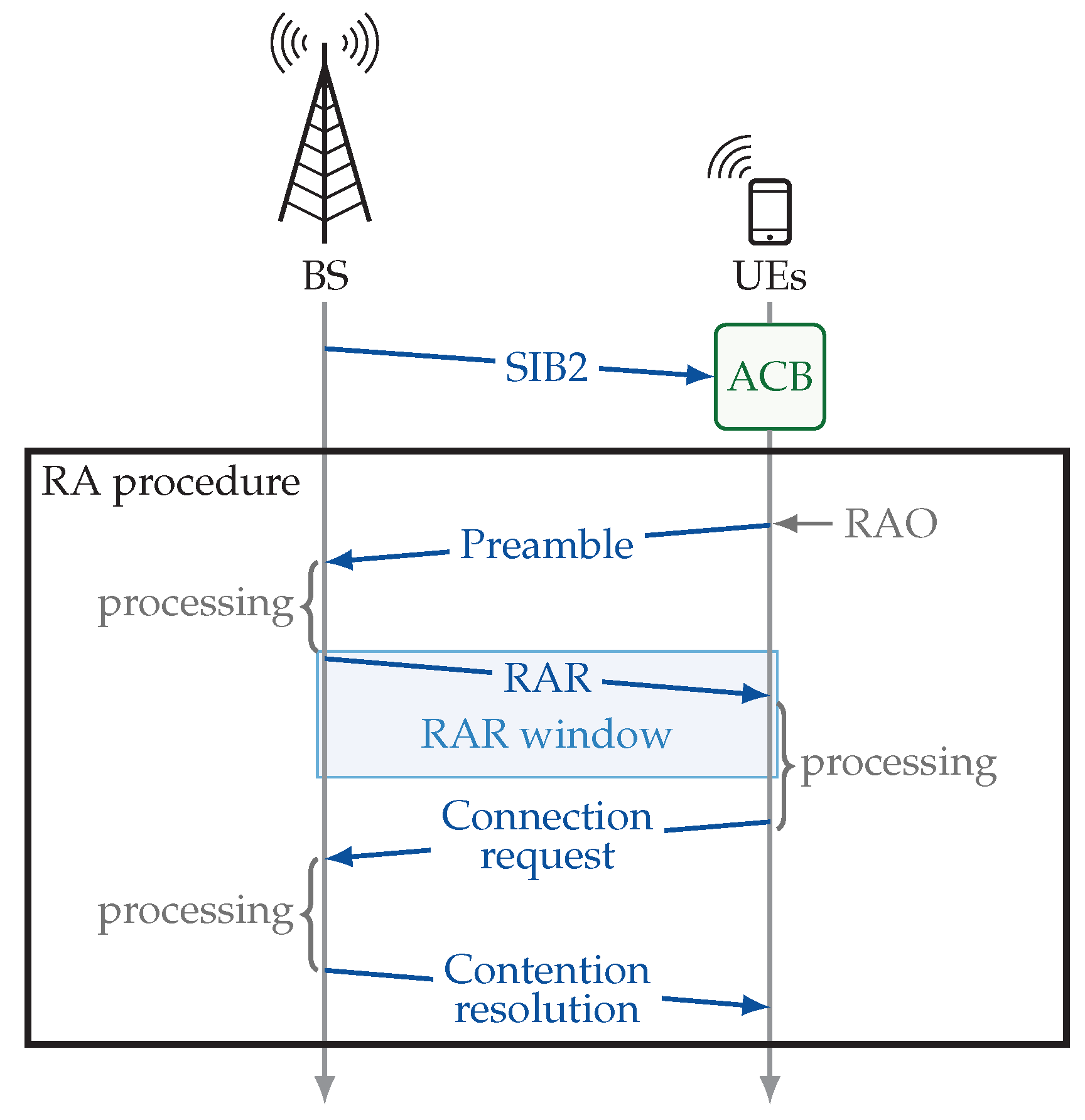
This section describes the random access (RA) as defined in the 3GPP standards. It comprises the access control and the contention-based RAP [1,20]. Throughout this study, the ACB, as defined in the 3GPP standards [1], is studied and we assume no other access control scheme is implemented. Figure 1 provides a brief description of the RA in 3GPP networks with the ACB scheme.

The first step for a UE to switch from idle to connected mode is to acquire the network configuration parameters. Once these have been obtained, the UE is subject to the ACB scheme and, finally, it performs the RAP. The network operates in a time-slotted channel in which the minimum unit for scheduling is the subframe.

The configuration parameters are broadcast by the cellular base station (BS) through the System Information Blocks (SIBs). The SIB1 includes, among other parameters, the periodicity of other SIBs in the parameter $si-Periodicity\in \{80,160,\cdots ,5120\}$ ms [1]. The SIB2 includes some basic parameters such as the periodicity of the time/frequency resources in which preamble transmissions are allowed $t_{\mathrm{rao}}$ (known as random access opportunities, RAOs) and the barring parameters [1,4,5,21].

The jth SIB2 transmission includes a barring rate $p_{\mathrm{acb}}\left(j\right)$ and a mean barring time $t_{\mathrm{acb}}\left(j\right)$ [1]. Only special categories of high-priority UEs may not be subject to the ACB scheme. The rest of the UEs subject to the ACB scheme must perform a barring check before initiating the RAP (i.e., before the transmission of their first preamble) as described in Algorithm 1 [1,22].

Algorithm 1 Access class barring (ACB) scheme.

1: repeat 2:  Acquire the mean barring time $t_{\mathrm{acb}}\left(j\right)$ and barring rate $p_{\mathrm{acb}}\left(j\right)$ broadcast in the jth SIB2. 3:  Generate $\mathcal{U}\left[0,1\right)\equiv$ a random number with uniform distribution between 0 and 1. 4:  if $\mathcal{U}\left[0,1\right)\le p_{\mathrm{acb}}\left(j\right)$ then 5:   Initiate the RAP. 6:  else 7:   Generate a new $\mathcal{U}\left[0,1\right)$. 8:   Select the barring time as $$t_{\mathrm{barred}}=\left(0.7+0.6\mathcal{U}\left[0,1\right)\right)t_{\mathrm{acb}}\left(j\right).$$ (1) 9:   Wait for $t_{\mathrm{barred}}$. 10:  end if 11: until the RAP is initiated.

UEs that succeed in a barring check are no longer subject to the ACB scheme [23] and proceed to perform the RAP as follows.

Preamble: Each UE randomly selects one out of the r available preambles and sends it towards the BS in a RAO through the random access channel (RACH). Multiple UEs can access the BS in the same RAO using different preambles due to their orthogonality. As a result, BS decodes the preambles transmitted without (wireless channel) errors by exactly one UE.

In this study, we assume the BS cannot decode preambles transmitted by multiple UEs simultaneously; we refer to these as collided preambles. This assumption goes in line with the 3GPP recommendations for the performance analysis of the RACH [2] and with most of the literature [3,14,15,24,25,26,27]. The interested reader may refer to [12] for details on the two main assumptions related to collisions during the RAP and their impact on performance.

Next, the UE waits for a predefined time window, known as the RA response (RAR) window, to receive a RAR message from the BS.

RAR: The BS computes an identifier for each successfully decoded preamble and sends the RAR message through the physical downlink control channel (PDCCH). It includes, among other data, uplink grants for the transmission of the next message, Msg3. Up to one RAR message can be sent per subframe, but it may contain several uplink grants; each of which is associated with a successfully decoded preamble.

The PDCCH resources are limited, so a maximum of $n_{\mathrm{ug}}$ uplink grants can be sent within a RAR window. Since up to three uplink grants can be sent per subframe in a RAR message, the number of available uplink grants per RAR window depends on its length.

Connection request and contention resolution: After receiving the corresponding uplink grant, the UEs schedule the transmission of the connection request message (Msg3) to the BS through dedicated resources. Then, the BS responds to each connection request with a contention resolution message (Msg4). The transmission of both of these messages is protected by a hybrid automatic repeat request (HARQ) mechanism.

The maximum number of allowed preamble transmissions for each UE is broadcast by the BS through the SIB2 [1]. Access failure can occur, for example, due to a preamble collision or to wireless channel errors during contention resolution. Whenever an access failure occurs, and if the maximum number of preamble transmissions has not been reached, the UE waits for a random backoff time (determined by the backoff indicator); then, it randomly selects and transmits a new preamble at the next RAO.

3. Access Class Barring Configuration (ACBC) Scheme

This section describes the structure of our ACBC scheme and the configuration of the selected filtering methods. It is important to emphasize our ACBC scheme, first introduced in [8], was designed to operate under the 3GPP specifications, hence, it can be directly implemented in 4G and 5G networks.

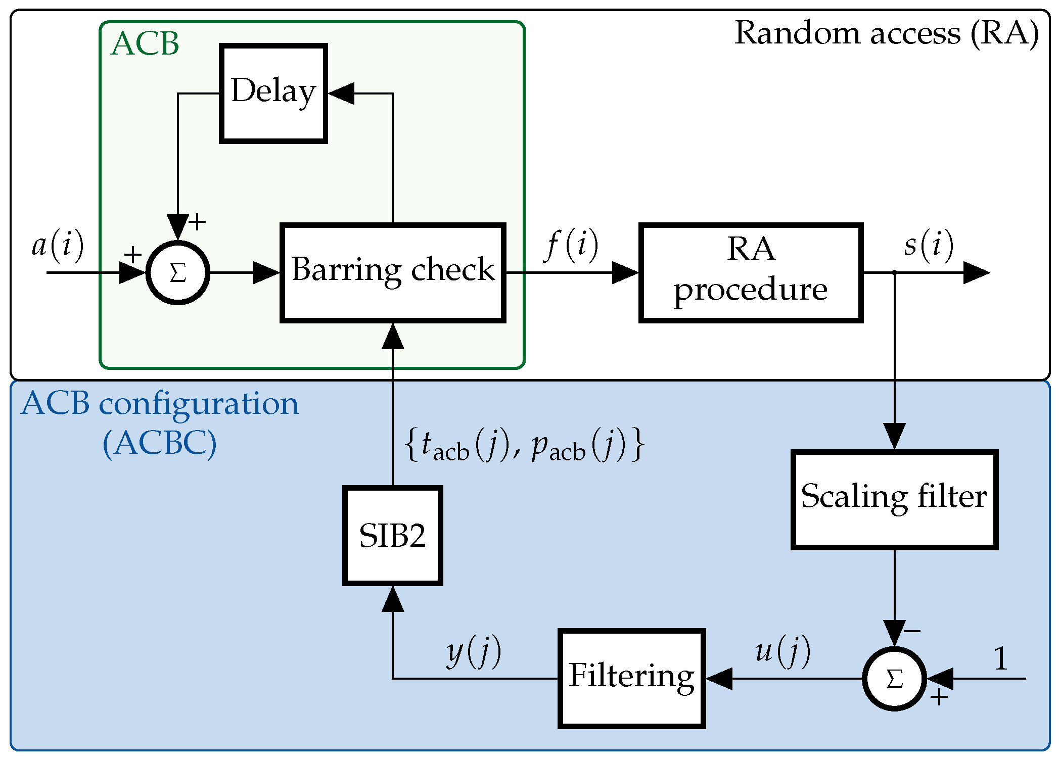
Figure 2 illustrates the block diagram that describes the operation of the RAP with our ACBC scheme. Two main blocks are clearly identified in the figure: the RA and the ACBC scheme. The RA, depicted in the upper part of Figure 2, operates as described in Section 2.

Let $a\left(i\right)$ be the number of UEs that attempt to switch from idle to connected mode for the first time at the ith RAO; these UEs are subject to the ACB scheme. Hereafter we refer to $a\left(i\right)$ simply as the UE arrivals.

Next, let $f\left(i\right)$ be the number of UEs whose barring check at the ith RAO is successful. These UEs begin the RAP at the ith RAO; hence, $f\left(i\right)$ is also the number of UEs whose first preamble is transmitted at the ith RAO. Finally, $s\left(i\right)$ is the number of UEs that will receive an uplink grant at the ith RAR window. That is, as a response to a preamble transmitted at the ith RAO. Therefore, the discrete time index i stands for the epoch number. The epoch duration is one RAO since the RA is performed at each and every RAO.

The lower part of Figure 2 depicts the structure of our ACBC scheme, where the BS calculates the barring parameters: mean barring time $t_{\mathrm{acb}}\left(j\right)$ and barring rate $p_{\mathrm{acb}}\left(j\right)$ that will be broadcast through the jth SIB2. The SIB2 is broadcast once every $t_{\mathrm{si}}$ RAOs, hence, these parameters are adapted according to the perceived access intensity throughout this period. As such, the discrete time index j stands for the epoch number when the epoch duration is $t_{\mathrm{si}}$ RAOs. Therefore, the ACBC scheme operates at a time scale that is $t_{\mathrm{si}}$ times greater than that of the RA block. Specifically, the jth SIB2 is broadcast at the $i=\left(j{t}_{\mathrm{si}}\right)$th RAO. Therefore, the barring parameters remain constant from the $\left(j{t}_{\mathrm{si}}+1\right)$th until the $\left(\left(j+1\right)t_{\mathrm{si}}\right)$th RAO. Throughout this study we assume $t_{\mathrm{acb}}\left(j\right)$ is selected beforehand and remains fixed throughout the operation of the network. Hence, the latter is simply denoted as $t_{\mathrm{acb}}$. In the following, we describe the process to calculate $p_{\mathrm{acb}}\left(j\right)$.

The BS calculates the ratio of idle to available resources immediately before the jth SIB2 transmission. For this, let $n\left(i\right)$ be the number of contending UEs (i.e., the total number of preamble transmissions) at the ith RAO. Please observe the number of successful preambles at an arbitrary RAO i is a random variable. From there, the theoretical PRACH (uplink) capacity can be defined as the maximum expected value of the latter random variable for a given number of available preambles r and for any $n\left(i\right)\in {\mathbb{R}}_{\ge 0}$. The PRACH capacity is achieved when the number of contending UEs is

$$n^{\ast }\left(i\right)={\left[log\left(\frac{r}{r-1}\right)\right]}^{-1}$$

(2)

and is calculated by Lin et al. [15] as

$$c\left(r\right)=n^{\ast }\left(i\right){\left(1-\frac{1}{r}\right)}^{n^{\ast }\left(i\right)-1}.$$

(3)

Next, let $c\left(r,n_{\mathrm{ug}}\right)$ be the theoretical capacity of the channels involved in the RAP: PRACH and PDCCH. The capacity of the PDCCH is exclusively determined by the number of available uplink grants per RAR window $n_{\mathrm{ug}}$ [2]. Hence, the capacity of the RAP is the minimum between the PRACH capacity and the PDCCH capacity,

$$c\left(r,n_{\mathrm{ug}}\right)=min\left\{c\left(r\right),n_{\mathrm{ug}}\right\}.$$

(4)

We refer to $c\left(r,n_{\mathrm{ug}}\right)$ simply as the RAP capacity.

With this information, the ratio of idle to available resources is calculated immediately before the jth SIB2 transmission (i.e., at the $\left(j{t}_{\mathrm{si}}\right)$th RAO) by means of the scaling filter block and the comparator shown in the bottom right corner of Figure 2 as

$$u\left(j\right)=1-{\mathit{h}}^{\mathsf{T}}\mathit{s}\left(j\right)$$

(5)

where $\mathit{h}=\left[h_0,h_1,\cdots ,h_{t_{\mathrm{si}}-1}\right]$ is the column vector of coefficients of the scaling filter

$$h_m=\frac{1}{t_{\mathrm{si}}c\left(r,n_{\mathrm{ug}}\right)},\mathrm{for}m\in \{0,1,\cdots ,t_{\mathrm{si}}\}$$

(6)

and $\mathit{s}\left(j\right)=\left[s\left(j{t}_{\mathrm{si}}\right),s(j{t}_{\mathrm{si}}-1),\cdots ,s(j{t}_{\mathrm{si}}-t_{\mathrm{si}})\right]$ is the vector that contains the number of uplink grants assigned at each of the $t_{\mathrm{si}}$ RAOs within the SIB2 period. Next, $u\left(j\right)$ serves as the input to the filtering process, whose output $y\left(j\right)$ is used to calculate the barring rate for the jth SIB2 broadcast interval

$$p_{\mathrm{acb}}\left(j\right)=min\left\{y\left(j\right),1\right\}.$$

(7)

Hence, $p_{\mathrm{acb}}\left(j\right)$ decreases with the ratio of idle to available resources. This increases the probability of delaying the beginning of the RAP when most of the resources have been utilized.

The filtering block in our ACBC scheme (at the bottom of Figure 2) is generic, which means different filtering methods can be implemented at this point. In the following, we describe three possibilities: two adaptive filtering algorithms and FIR filters with fixed coefficients.

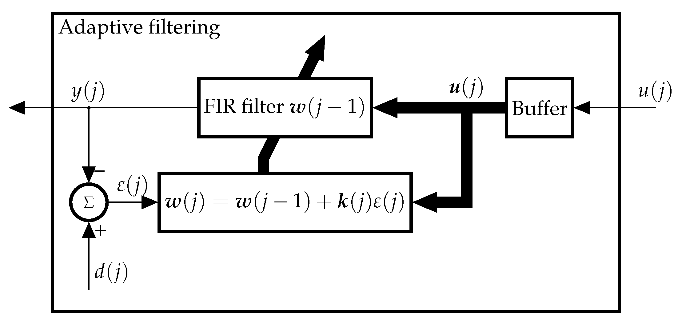
3.1. Recursive Least-Squares (RLS) Algorithm

The RLS is an adaptive algorithm that minimizes the total squared error between its output and the desired response. In particular, it is a recursive implementation of the method of least squares. The RLS can be derived from the least-mean square (LMS) algorithm, described in the next subsection, and is renowned for its fast rate of convergence. For instance, the rate of convergence of the RLS can be up to an order of magnitude faster than that of the LMS. In exchange, its numerical complexity is in the order of $\mathcal{O}\left(M^2\right)$, which is higher than that of the LMS. Nevertheless, the mathematical formulation and implementation of the RLS is relatively simple [28].

The internal structure of the RLS algorithm is illustrated in Figure 3. A buffer has been incorporated to clearly illustrate that the ratio of idle resources during the last M SIB2 intervals

$$\mathit{u}\left(j\right)=\left[u\left(j\right),u(j-1),\cdots ,u(j-M+1)\right]$$

(8)

is the input to the algorithm. That is, a single value of $u\left(j\right)$ is the input to the buffer as indicated by the thin arrow, and the output of the buffer is a vector, as indicated by the thick arrows.

The RLS is summarized in Algorithm 2, and consists of a filtering and an adaptive process.

In the filtering process, the output of the FIR filter $y\left(j\right)$ is computed from $\mathit{u}\left(j\right)$.

In the adaptive process, the output $y\left(j\right)$ is compared to the desired response $d\left(j\right)$ to adapt the weights of the FIR filter

$$\mathit{w}\left(j\right)=\left[w_0\left(j\right),w_1\left(j\right),\cdots ,w_{M-1}\left(j\right)\right].$$

(9)

The parameter $\epsilon \left(j\right)$ is the a priori error, which represents an estimate of the desired response $d\left(j\right)$ based on the old least-squares estimate of $\mathit{w}\left(j-1\right)$. It is essential to emphasize that $\epsilon \left(j\right)$ is different to the a posteriori estimation error $e\left(j\right)$, calculated in the LMS algorithm (see next subsection).

Regarding the configuration of the RLS in our ACBC scheme, the desired response is set to be $d\left(j\right)=1$ for all j. By doing so, the RLS algorithm is set to minimize the distance between the output $y\left(j\right)$ and its maximum value, $d\left(j\right)=1$, which in turn “pulls” the output toward the aforementioned maximum value. This increases the barring rate $p_{\mathrm{acb}}\left(j\right)$ and, in turn, reduces the access delay of UEs. This effect will be described in detail on page 16.

The RLS algorithm has two parameters that must be selected empirically, the regularization parameter $\delta$ and the forgetting factor $\lambda$. The latter determines the rate at which the effect of the previous inputs on the algorithm is minimised. There is no exact method to select $\delta$ nor $\lambda$. However, the following recommendations exist [28].

• Regularization parameter $\delta$: Select a small positive value when the input (in our case $u\left(j\right)$) is relatively high with respect to its sudden variations. Select a large positive value otherwise.
• Forgetting factor $\lambda$: Select a positive value that is close to, but less than, 1. This ensures that past the values of the input $u\left(j\right)$ are forgotten by the algorithm. On the other hand, $\lambda =1$ corresponds to the method of least squares.

The beginning of Section 4 focuses on finding adequate values for $\delta$ and $\lambda$.

Algorithm 2 RLS adaptive algorithm.

Require: the number of filter coefficients M Require: regularization parameter $\delta >0$ Require: forgetting factor $\lambda$ 1: Initialize the vector of filter coefficients $\mathit{w}\left(0\right)$ and the input vector $\mathit{u}\left(0\right)$ as $$w_m\left(0\right)=u\left(-m\right)=0,m\in \{0,1,\cdots ,M-1\}$$ (10) 2: Initialize the inverse correlation matrix $\mathit{P}\left(0\right)={\delta }^{-1}\mathit{I}$ 3: for all$j=1,2,\dots$do 4: Filtering process: $$y\left(j\right)={\mathit{w}}^{\mathsf{T}}(j-1)\mathit{u}\left(j\right)$$ (11) 5: Adaptive process: $$\begin{array}{cc}\hfill \mathit{k}\left(j\right)& =\frac{{\lambda }^{-1}\mathit{P}\left(j-1\right)\mathit{u}\left(j\right)}{1+{\lambda }^{-1}{\mathit{u}}^{\mathsf{T}}\left(j\right)\mathit{P}\left(j-1\right)\mathit{u}\left(j\right)}\hfill \end{array}$$ (12a) $$\begin{array}{cc}\hfill \epsilon \left(j\right)& =d\left(j\right)-y\left(j\right)\hfill \end{array}$$ (12b) $$\begin{array}{cc}\hfill \mathit{w}\left(j\right)& =\mathit{w}(j-1)+\mathit{k}\left(j\right)\epsilon \left(j\right)\hfill \end{array}$$ (12c) $$\begin{array}{cc}\hfill \mathit{P}\left(j\right)& ={\lambda }^{-1}\mathit{P}\left(j-1\right)-{\lambda }^{-1}\mathit{k}\left(j\right){\mathit{u}}^{\mathsf{T}}\left(j\right)\mathit{P}\left(j-1\right)\hfill \end{array}$$ (12d) 6: end for

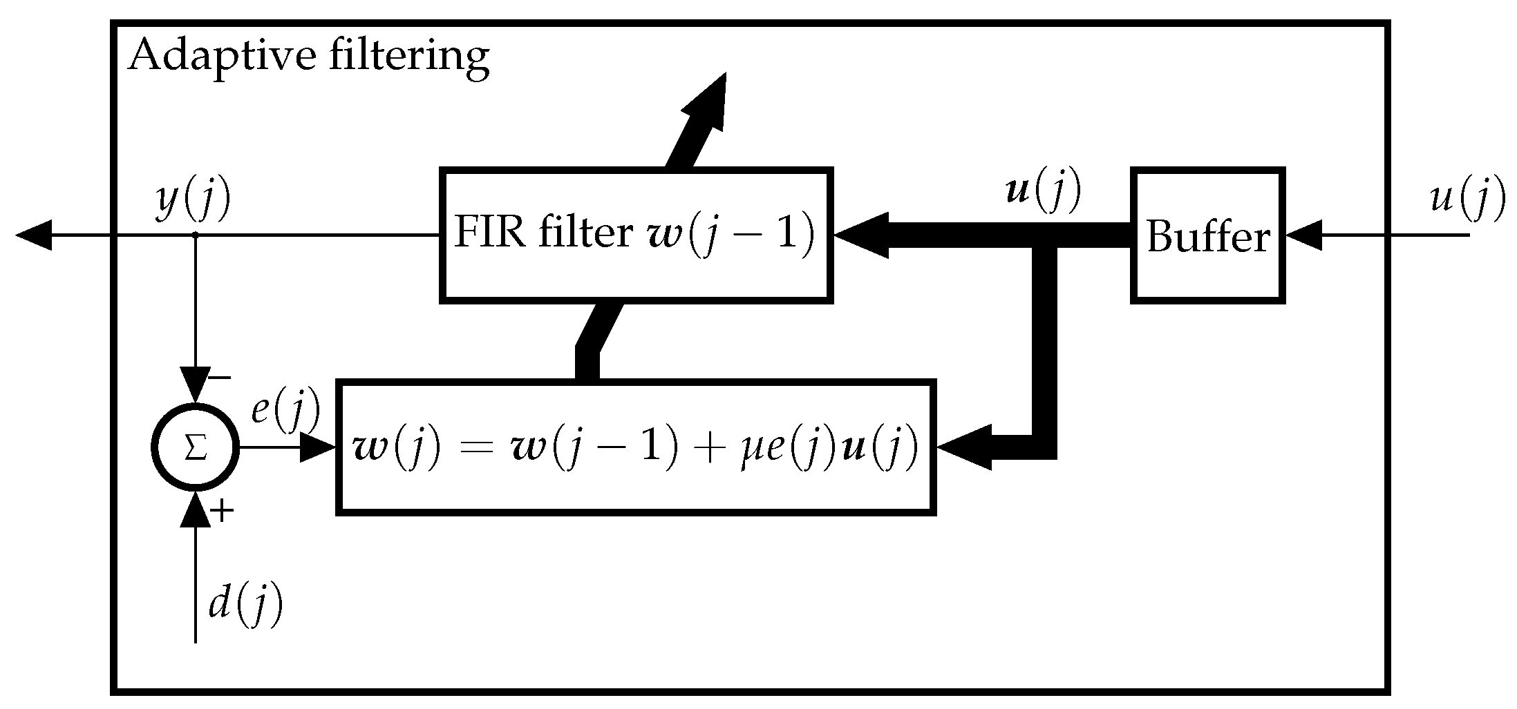
3.2. Least-Mean Square (LMS) Algorithm

The LMS algorithm is widely used because of its simplicity and numerical robustness [28]. Concretely, the complexity of the LMS scales linearly with the filter length M. The LMS is an application of the method of stochastic gradient descent, hence, it belongs to a different family of algorithms to that of the RLS. The internal structure of the LMS is depicted in Figure 4 and Algorithm 3 summarizes its operation.

Algorithm 3 LMS adaptive algorithm.

Require: the number of filter coefficients M Require: the adaptation step size $\mu$ 1: Initialize the vector of filter coefficients $\mathit{w}\left(0\right)$ and the input vector $\mathit{u}\left(0\right)$ as $$w_m\left(0\right)=u\left(-m\right)=0,m\in \{0,1,\cdots ,M-1\}$$ (13) 2: for all$j=1,2,\cdots$do 3:   Select the desired response $d\left(j\right)$ 4:   Filtering process: $$y\left(j\right)={\mathit{w}}^{\mathsf{T}}(j-1)\mathit{u}\left(j\right)$$ (14) 5:   Adaptive process: $$\begin{array}{cc}\hfill e\left(j\right)& =d\left(j\right)-y\left(j\right)\hfill \end{array}$$ (15a) $$\begin{array}{cc}\hfill \mathit{w}\left(j\right)& =\mathit{w}(j-1)+\mu e\left(j\right)\mathit{u}\left(j\right)\hfill \end{array}$$ (15b) 6: end for

As with the RLS, the LMS comprises a filtering and an adaptive process. An important difference between these two algorithms is that the output $y\left(j\right)$ is compared to the desired response $d\left(j\right)$ to obtain the error $e\left(j\right)$ in the LMS, whereas the a priori error $\epsilon$ is calculated in the RLS.

The correct selection of the rate of adjustment $\mu$ is essential for the LMS to be stable. In particular, the value of $\mu$ must be selected to satisfy

$$0<\frac{1}{2}\mu {\parallel \mathit{u}\left(j\right)\parallel }^2<1,\mathrm{for}\mathrm{all}\mathit{u}\left(j\right)$$

(16)

where $\parallel ·\parallel$ is the Euclidean norm operator.

Two different configurations of the LMS algorithm are considered: an adaptive line enhancer (ALE) and a “pulling” ALE (PALE). In the ALE, the primary input is a delayed version of $\mathit{u}\left(j\right)$, namely $\mathit{u}(j-1)$, while the desired output is set to $d\left(j\right)=u\left(j\right)$. In the PALE, the primary input is simply $u\left(j\right)$ and the desired output is set to $d\left(j\right)=1$ for all j. The latter configuration has a similar effect on the filter output as the one described above for the RLS configuration.

3.3. Simple Low-Pass FIR Filter

Besides investigating the benefits of our ACBC scheme with the two previously described adaptive filter algorithms, we also consider the inclusion of a simple FIR filter with fixed weights $w_m$. We refer to this as the low-pass filtering (LPF) method.

The filter weights must be chosen to ensure the following two conditions are met.

$$\sum _{m=0}^{M-1}{w}_m=1$$

(17a)

$$w_m>0,\mathrm{for}\mathrm{all}m\in \{0,1,\dots ,M-1\}.$$

(17b)

For this, let $\rho$ be the degree of the decreasing polynomial function that determines the fixed weights of the filter. Naturally, the rapidness of the response of the fixed filter to sudden changes in the input $u\left(j\right)$ increases with $\rho$, but so does its sensitivity. In other words, the selection of $\rho$ creates a trade-off between the responsiveness and the stability of the filter output.

In particular, we choose the filter weights as

$$w_m={\left(M-m\right)}^{\rho }{\left(\sum _{m=0}^{M-1}{\left(M-m\right)}^{\rho }\right)}^{-1}={\left(M-m\right)}^{\rho }{\left(\sum _{\ell =1}^M{\ell }^{\rho }\right)}^{-1};$$

(18)

where ${\sum }_{\ell =1}^M{\ell }^{\rho }$ is the normalization factor.

3.4. Methodology

In this study, we aim to compare the tracking capabilities of the RLS adaptive algorithm to those of the LMS and simple fixed FIR filters in a transient environment: the traffic model 2 defined by the 3GPP [2]. The latter represents a highly synchronized mMTC scenario, in which the UE arrivals follow a $\mathrm{Beta}\left(3,4\right)$ distribution over 10 s. Several studies have confirmed the traffic model 2 leads to severe congestion if no access control scheme is implemented [2,3,4,5,12,13].

Results presented in the following section were obtained by simulation. In particular, a C-based simulator is used, which closely replicates the arrival process of the UEs, the ACB scheme, and the RAP as described in the specifications [1,22]. In each simulation, the adaptive algorithm is initialized and the filter weights are stabilized (if applicable). Then, n = 30,000 UE arrivals are scheduled within the distribution period $t_{\mathrm{dist}}$ which begins at $i=0$. The jth SIB2 is broadcast at the $\left(j{t}_{\mathrm{si}}+i_r\right)$th RAO, where $i_r$ is a discrete random time shift, selected from a uniform distribution between 0 and $t_{\mathrm{si}}-1$. A simulation run is concluded when every UE has terminated the RA procedure. The number of simulation runs is set to the smallest number that ensures the cumulative results obtained up to the last simulation differ from those obtained up to the previous simulation by less than $0.01$ percent.

The first step in our analyses is to use a non-synchronized mMTC scenario, the traffic model 1, to identify an adequate configuration of the RLS algorithm. The traffic model 1 can be seen as a stationary scenario of finite duration with a low access intensity, in which UE arrivals follow a uniform distribution over 60 s. As such, the traffic model 1 (stationary scenario) is used to “train” the RLS algorithm to provide an adequate response in a transient scenario. For this, we set the UEs to ignore the ACB scheme and assess two main characteristics: the rate of convergence of the output of the filter and the relative amplitude of its variations with respect to the mean value. It is important to emphasize that similar trial and error approaches to set the configuration of adaptive algorithms are the most common in the practice, especially in transient scenarios [29]. The main characteristics of both traffic models are listed in

Table 1. Characteristics of the different traffic models defined by the 3GPP for the performance evaluation of the RAP [2].

Parameter	Traffic Model 1	Traffic Model 2
Number of UEs n	30,000	30,000
Distribution period $t_{\mathrm{dist}}\left(\mathrm{s}\right)$	60	10
Distribution over $t_{\mathrm{dist}}$	Uniform	$\mathrm{Beta}(3,4)$

.

In our experiments, we assume the most typical configuration of the RACH, as suggested by the 3GPP [2]. The number of available preambles is set to $r=54$; this is the most typical value for this parameter. Furthermore, it allows us to evaluate the RAP in a scenario in which the number of successful accesses is greatly affected by r, but also by the number of available uplink grants $n_{\mathrm{ug}}$. In addition, we assume the shortest possible period for the SIB transmissions, 80 ms. These values are listed in

Table 2. Parameters for the selected network configuration.

Parameter	Setting
Available preambles	$r=54$
Subframe length	1 ms
RAO periodicity	$t_{\mathrm{rao}}=5$ subframes
RAR window size	5 subframes
Available uplink grants per RAR window	$n_{\mathrm{ug}}=15$
Period of SIB transmissions	80 ms
SIB2 periodicity in RAOs	$t_{\mathrm{si}}=16$
Maximum number of preamble transmissions	10
Backoff indicator	20 ms
Detection probability for the kth preamble transmission	$P_d\left(k\right)=1-1/e^k$
Maximum number of Msg3 and Msg4 transmissions	5
Detection probability for Msg3 and Msg4	$0.9$

, along with other values selected for the most relevant configuration parameters.

To assess the benefits of the RLS algorithm, we test several values for parameter $\delta$ and $\lambda$, whereas other configuration parameters remain fixed. For example, $M=32$ is a widely used filter length that led to satisfactory results in our preliminary tests with the RLS algorithm. Furthermore, it is the filter length that maximizes the benefits of the LMS algorithm [19]. Therefore, it is selected throughout the remainder of the paper for every filter.

In addition, we select an intuitive value for the mean barring rate $t_{\mathrm{acb}}=1$ s among those available in the SIB2; as it will be seen throughout the following section, this value leads to a sufficiently high $P_s\ge 0.95$ for all the selected filtering methods under the traffic model 2. Certainly, an optimal value for this parameter could be selected, but it is out of the scope of this paper to optimize the performance of each of the studied filtering methods under the selected scenario. Furthermore, selecting a value higher than $t_{\mathrm{acb}}=1$ only causes a slight increase in the access delay when compared to the results presented in this paper. The interested reader may refer to [19], where our ACBC scheme with the LMS algorithm was optimized, and apply an analogous procedure for the RLS algorithm. The configuration parameters for the filtering methods studied in this paper are listed in

Table 3. Parameters for the selected filter configurations.

Filtering Method	Parameter	Setting
Common to all
	Number of filter coefficients	$M=32$
	Mean barring time	$t_{\mathrm{acb}}=1$ s
RLS
	Forgetting factor	$\lambda \in \{0.99,0.999,1\}$
	Regularization parameter	$\delta \in \{10,1,0.1,0.01,0.001\}$
	Primary input	$u\left(j\right)$
	Desired response	$d\left(j\right)=1$
LMS ALE
	Adaptation step size	$\mu =1/800$
	Primary input	$u(j-1)$
	Desired response	$d\left(j\right)=u\left(j\right)$
LMS PALE
	Adaptation step size	$\mu =1/800$
	Primary input	$u\left(j\right)$
	Desired response	$d\left(j\right)=1$
LPF
	Polynomial degree	$\rho \in \{0,1,2\}$

.

In particular, we are set to find configurations of the RLS and fixed FIR filters that successfully reduce the variations of $u\left(j\right)$ with the fastest possible convergence toward $\mathbb{E}\left[u\left(j\right)\right]$. Under the traffic model 1, n = 30,000 UE accesses are uniformly distributed within 60 s. Since RAOs occur once every $t_{\mathrm{rao}}=5$ subframes and the subframe duration is 1 ms, there are $i_{\mathrm{dist}}$ = 12,000 RAOs in the distribution period.

Let A be the random variable that defines the number of UE arrivals at an arbitrary RAO within the distribution period. Hence, $a\left(i\right)$, shown in Figure 2, is the outcome of a single experiment for random variable A at the ith RAO. Please observe $A\sim \mathrm{B}\left(n,1/i_{\mathrm{dist}}\right)$, hence, we have $\mathbb{E}\left[A\right]=n/i_{\mathrm{dist}}=2.5$. Since the intensity of access attempts under the traffic model 1 is considerably low when compared to the RAP capacity, the number of successful accesses per RAO $s\left(i\right)$ highly resembles that of UE arrivals (i.e., $s\left(i\right)\approx a\left(i\right)$, for all i). As a consequence, $\mathbb{E}\left[u\left(j\right)\right]$ can be approximated by substituting $\mathit{s}\left(i\right)$ with $\mathit{a}$, a column vector of length $t_{\mathrm{si}}$ whose entries are $\mathbb{E}\left[A\right]$, in (5).

$$\mathbb{E}\left[u\left(j\right)\right]\approx 1-{\mathit{h}}^{\mathsf{T}}\mathit{a}=1-\frac{\mathbb{E}\left[A\right]}{c\left(r,n_{\mathrm{ug}}\right)}$$

(19)

which gives $\mathbb{E}\left[u\left(j\right)\right]\approx 5/6$ for $r=54$. This value has been confirmed by simulation and by an analytical model [12].

4. Results

In this section, we assess the benefits of our ACBC scheme with different filtering methods. As a starting point, we find adequate values for the regularization parameter $\delta$ and the forgetting factor $\lambda$, which determine the response of the RLS algorithm. Next, we briefly study the response of the LPF method (fixed FIR filters) and of the LMS algorithm. Next, we assess the benefits provided by the different filtering methods under the traffic model 2, when compared to an ACB scheme with fixed parameters (static ACB) and to our ACBC scheme with no filtering (i.e., where $y\left(j\right)=u\left(j\right)$). The section concludes with the comparison of the response of the different filtering methods under the traffic model 2.

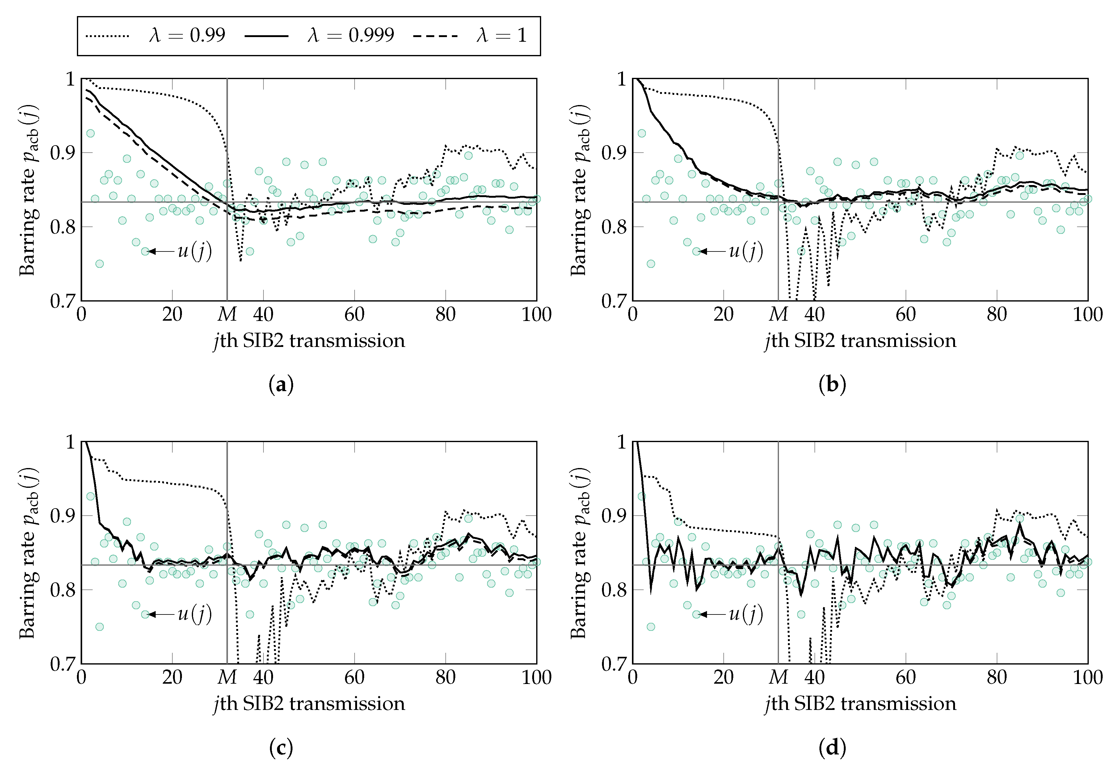
Adequate values for parameters $\delta$ and $\lambda$ are selected by observing the response of the algorithm. The latter is illustrated in Figure 5 for $\delta \in \{0.001,0.01,0.1,1\}$ and $\lambda \in \{0.99,0.999,1\}$, given $r=54$, along with the calculated $u\left(j\right)$. Clearly, the response is not adequate with $\lambda =0.99$ as $p_{\mathrm{acb}}\left(j\right)$ presents a drastic drop around $j=M$, hence, the response of the RLS is not stable. On the other hand, the difference in the response between selecting $\lambda =0.999$ and $\lambda =1$ is minimal; both of these values of $\lambda$ greatly reduce the variations of $p_{\mathrm{acb}}\left(j\right)$ given a sufficiently low value of $\delta$ is selected, for example, $\delta =0.001$. Figure 5 shows $\delta =0.01$ is also an acceptable candidate for the regularization parameter, whereas higher values of $\delta$ should be avoided, as the amplitude of variations of $p_{\mathrm{acb}}\left(j\right)$ is high when compared to its mean.

It has been observed in the literature that parameter $\lambda$ plays a similar role in the RLS algorithm as the complement of parameter $\mu$ in the LMS algorithm [28]. In our previous studies we observed $\mu =1/800$ is an adequate value for the adaptation step size in our ACBC scheme. Hence, results presented in Figure 5 confirm the relation between $\lambda$ and $\mu$, as an adequate response is obtained with $\lambda =0.999\approx 1-1/800=1-\mu$. The latter value of $\lambda$ is selected throughout the remainder of the paper, in combination of $\delta =0.001$. As it can be seen, $p_{\mathrm{acb}}\left(j\right)$ with this combination converges toward $\mathbb{E}\left[u\left(j\right)\right]$ around $j=M$.

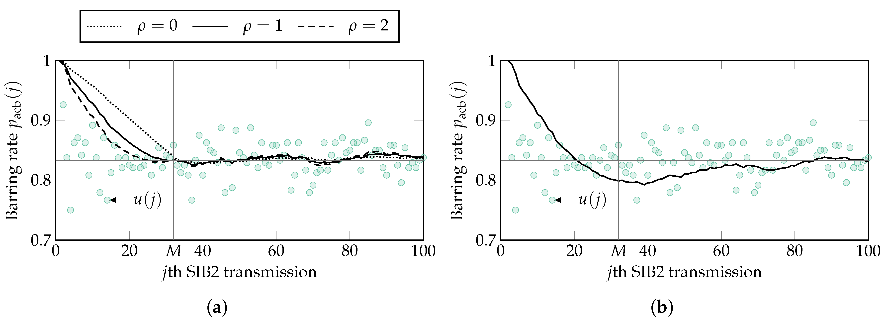
Regarding the LPF method, it is immediate to see in Figure 6 that $p_{\mathrm{acb}}\left(j\right)$ converges toward $\mathbb{E}\left[u\left(j\right)\right]$ at exactly $j=M$ for $\rho =0$, and the rate of convergence increases slightly with $\rho$. It is also interesting to observe that the $p_{\mathrm{acb}}\left(j\right)$ calculated with the RLS, given $\lambda =0.999$ and $\delta =0.1$, shown in Figure 5b, is highly similar to that of the LPF method. On the other hand, the $p_{\mathrm{acb}}\left(j\right)$ calculated with the LMS presents a different behavior to both the RLS and LPF methods. For example, $p_{\mathrm{acb}}\left(M\right)<\mathbb{E}\left[u\left(j\right)\right]$ and converges toward $\mathbb{E}\left[u\left(j\right)\right]$ approximately until $j=100$.

Next, we investigate whether the difference in the response of the filters provides different benefits to our ACBC scheme. For this, we consider three key performance indicators (KPIs):

• Success probability, defined as the probability to successfully complete the RAP. The minimum success probability considered as acceptable is $0.95$. Hence, the main goal of our ACBC scheme is to guarantee that more than 95% of the UEs successfully complete the RAP.
• Access delay, defined as the time elapsed since the arrival of a specific UE and the successful completion of its RAP. This KPI is assessed in terms of the 95th percentile. That is, the delay of 95% of the UEs that successfully complete the RAP is lower than, or equal, to the reported value.
• Number of preamble transmissions to successfully complete the RAP. This KPI is assessed in terms of its expected value.

It is important to emphasize that the success probability under the traffic model 2 with no implemented ACB scheme is only $0.313$, which is poor. In addition, the benefits of our ACBC scheme are minor when no filtering is performed and $y\left(j\right)=u\left(j\right)$. Specifically, the success probability with $t_{\mathrm{acb}}=1$ s and no filtering is only $0.419$, which is still unacceptable. The reason for such a poor performance is that the UE arrivals and the number of successful accesses per RAO present high variations with respect to their mean value. These variations remain present in $u\left(j\right)$ and, naturally, in $p_{\mathrm{acb}}\left(j\right)$. On the other hand, filtering away these variations in $u\left(j\right)$ leads to a stable $p_{\mathrm{acb}}\left(j\right)$ that is closely related to the intensity of UE accesses in a larger time scale to that of the SIB2 period.

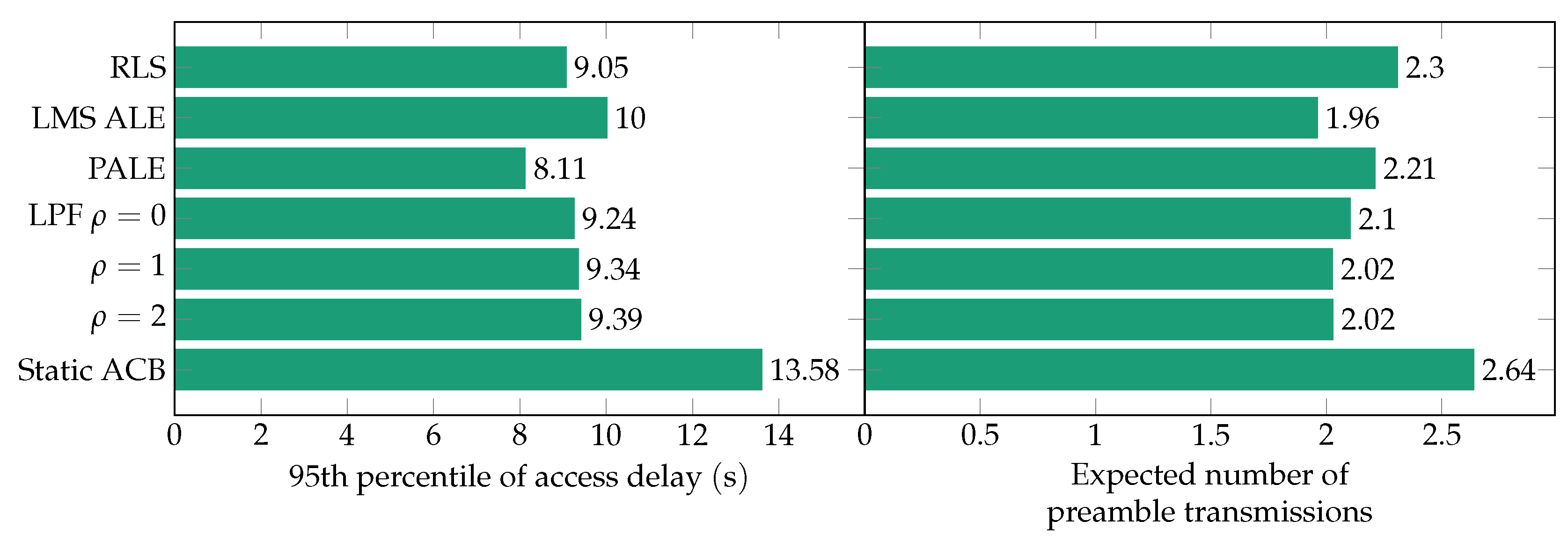
Figure 7 shows the 95th percentile of access delay and the expected number of preamble transmissions for the studied filtering methods. The success probability obtained with our ACBC scheme with each of the filtering methods included in Figure 7 is higher than $0.985$, hence, the difference between them, in this KPI, is negligible. In contrast, the success probability under the traffic model 2 without ACB scheme is only $0.313$. For benchmark purposes, Figure 7 also includes the KPIs obtained with the optimal configuration of a static ACB. The optimal configuration for the latter is defined as the combination of fixed barring parameters that leads to a success probability of $0.95$ or higher with the shortest 95th percentile of access delay. In particular, we found the optimal configuration of the static ACB to be $p_{\mathrm{acb}}=0.31$ and $t_{\mathrm{acb}}=1.75$ s, which yields a success probability of $0.95$.

As it can be seen, regardless of the selected filtering method, the 95th percentile of access delay and the expected number of preamble transmissions are reduced by more than 26% and 12%, respectively, when compared to the optimal static ACB implementation. It can also be seen in Figure 7 that the different values of $\rho$ for the LPF method have a minimal impact on performance. Specifically, the difference in each of the two KPIs shown in the figure for the different valued of $\rho$ is less than 4%.

On the other hand, there is a significant difference between the KPIs obtained with each of the adaptive algorithm configurations. In particular, the ALE leads to the longest access delay but to the lowest number of transmissions, whereas the opposite occurs with the PALE. The RLS leads to an access delay that is in between both LMS configurations, but to the highest number of preamble transmissions. This difference is caused by the “pulling” effect of the PALE and RLS algorithms, which is absent from the ALE.

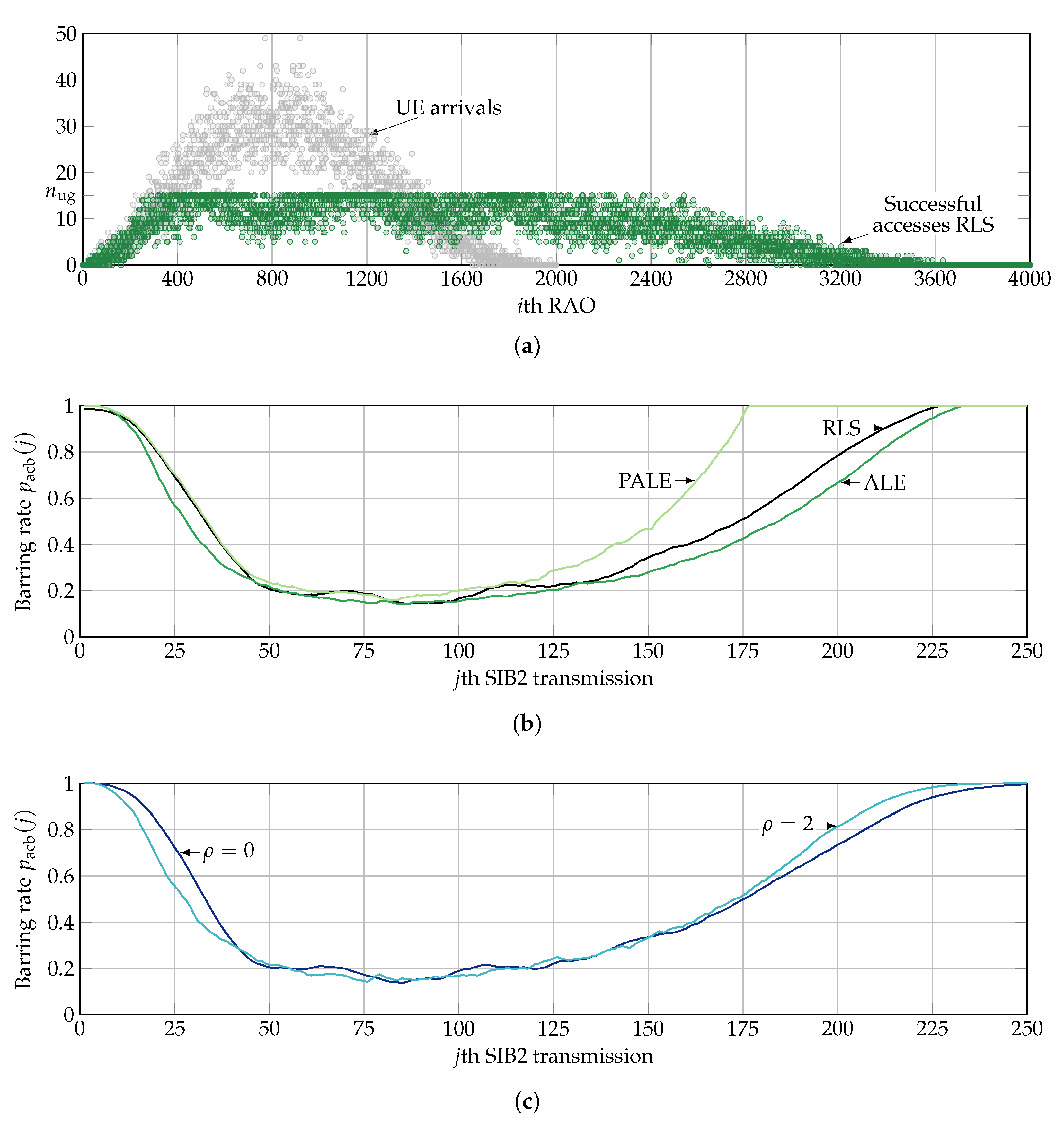
Figure 8 clearly illustrates the difference in the $p_{\mathrm{acb}}\left(j\right)$ calculated with the ALE, PALE, RLS, and LPF methods. The number of UE arrivals and successful accesses at each RAO with the RLS algorithm are also illustrated as a reference in Figure 8a. From this figure, it can be seen the number of UE accesses and successful accesses per RAO are highly variable. Furthermore, the number of successful accesses per RAO closely follows that of UE arrivals in the interval $0\le i\le 343$. Then, for $i\ge 343$, the number of successful accesses approaches $n_{\mathrm{ug}}$. This behavior is highly desirable, as it maximizes the utilization of resources and, in turn, reduces the access delay of UEs.

Next, Figure 8b,c exhibit that the LMS algorithm with the ALE configuration operates as a low-pass filter with output $p_{\mathrm{acb}}\left(j\right)$. That is, the calculated $p_{\mathrm{acb}}\left(j\right)$ with the ALE configuration highly resembles that with the LPF method with both $\rho \in \{0,2\}$. On the other hand, the PALE and the RLS “pull” the latter toward $d\left(j\right)=1$. As a consequence, the $p_{\mathrm{acb}}\left(j\right)$ calculated with the PALE and RLS are higher than those with the ALE and LPF methods. However, it is important to observe that the “pulling” effect is greater for the PALE than for the RLS. For instance, $p_{\mathrm{acb}}\left(j\right)$ increases more rapidly for the PALE than for the RLS as the number of UE arrivals drops (i.e., after the 2000th RAO, which corresponds to the 150th SIB2 transmission). The reason for this effect is the rapid response of the RLS, which converges more rapidly toward $\mathbb{E}\left[u\left(j\right)\right]$, calculated with the M most recent values of $u\left(j\right)$. As a result, the benefits provided by the RLS are in between those provided by the ALE and the PALE.

On the other hand, the calculated $p_{\mathrm{acb}}\left(j\right)$ with both $\rho \in \{0,2\}$ is closely similar in the period $j\in \left[50,175\right]$, and the difference is observed when rapid changes in the number of successful accesses occur. Naturally, the rate of change of $p_{\mathrm{acb}}\left(j\right)$ with respect of $s\left(i\right)$ is more rapid for $\rho =2$ than for $\rho =0$. However, this difference is not evident in the 95th percentile of access delay, illustrated in Figure 7.

5. Conclusions

In this paper, we investigated the impact of implementing different filtering methods to our ACBC scheme under a typical mMTC scenario: the traffic model 2. The latter leads to severe congestion when no access control scheme is implemented.

Based on the behavior described in Section 4, it is safe to claim that our ACBC scheme can operate efficiently with several filtering methods, and its performance is compromised only if this process is omitted. That is, when compared to the optimal configuration of a static ACB scheme, our ACBC scheme can reduce the 95th percentile of access delay by more than 26%, while increasing the success probability and reducing the number of preamble transmissions with numerous filtering methods.

One of the main advantages of selecting an adaptive algorithm, such as the LMS and the RLS, is the “pulling” effect provided by setting the desired response to 1. By doing so, the access delay of UEs is further reduced. The latter is of utmost importance under scenarios in which the number of UE accesses is considerably low when compared to the RAP capacity, such as the traffic model 1. In these scenarios, an access control scheme is not needed and increasing the access delay of UEs may be counterproductive. On the other hand, correctly configuring the LMS and RLS algorithms is not straightforward and different methods to reduce the access delay in these scenarios exist. For example, the mean barring time can be set to be a function of the barring rate, hence reducing the barring time as the barring rate increases. Furthermore, if the access delay is not relevant at all, implementing a simple FIR filter in our ACBC scheme would be equally effective as implementing an adaptive algorithm, but the former eliminates the difficulty of selecting correct configuration parameters.