Reduced Computational Complexity Orthogonal Matching Pursuit Using a Novel Partitioned Inversion Technique for Compressive Sensing

 , ,
, , 
Abstract
:1. Introduction
2. Overview of SOMP Algorithm
2.1. Description of SOMP Algorithm
| Algorithm 1. Simultaneous orthogonal matching pursuit (SOMP). |
| Input: •ℝM×N: The measurement matrix • y ℝM×L: The multiple measurement vector Output: • ℝN×L: The estimate of original signal Variable: • m: The sparsity level of original signal x • r ℝM×L: The residue Initialize: , For ith iteration: 1. , where , and k is an index 2. 3. 4. Repeat process until i = m to generate the final estimate of the . |
2.2. Least Square (LS) Problem
3. Conditions of the Input Matrix in LS Problem
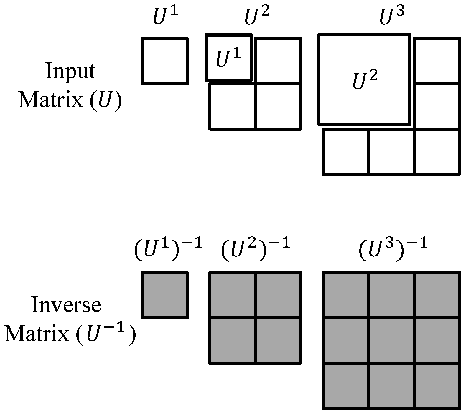
4. Proposed Partitioned Inversion
4.1. Conventional Partitioned Inversion
4.2. Proposed Partitioned Inversion
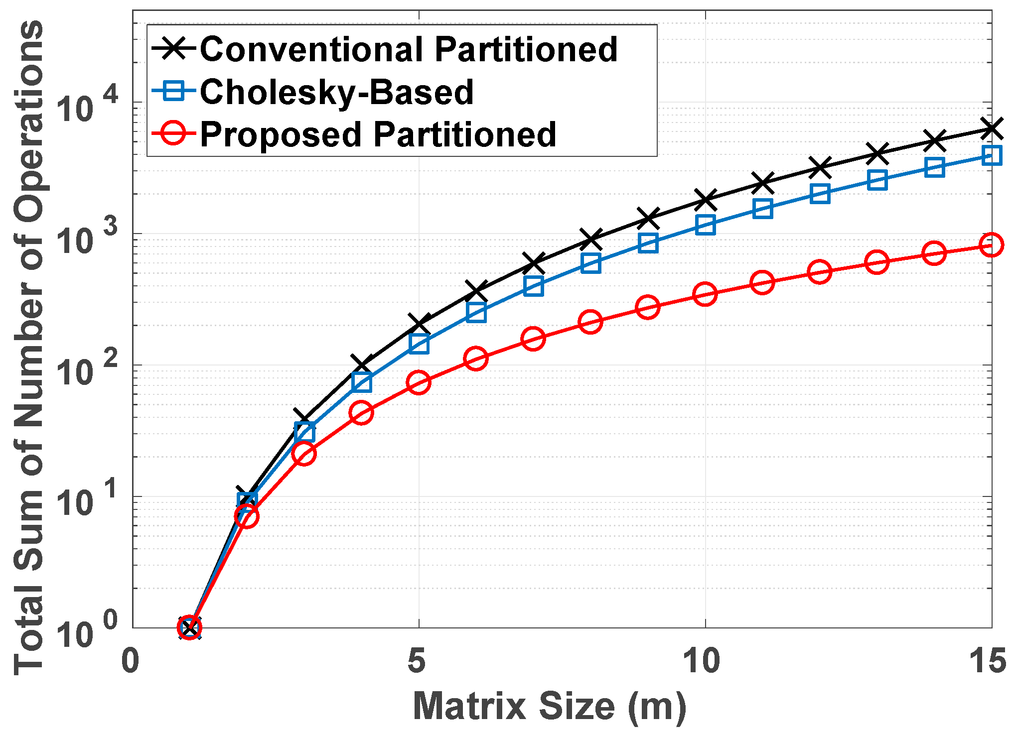
4.3. Computational Complexity for Proposed Partitioned Inversion
4.4. Proposed Partitioned Inversion for Multiple Supporter System
- Multiplication:
- Add/sub:
- Division:where n is the number of the supporter. Although the computation complexity becomes larger as n increases, the proposed inversion method can be applied to the multiple supporter system.
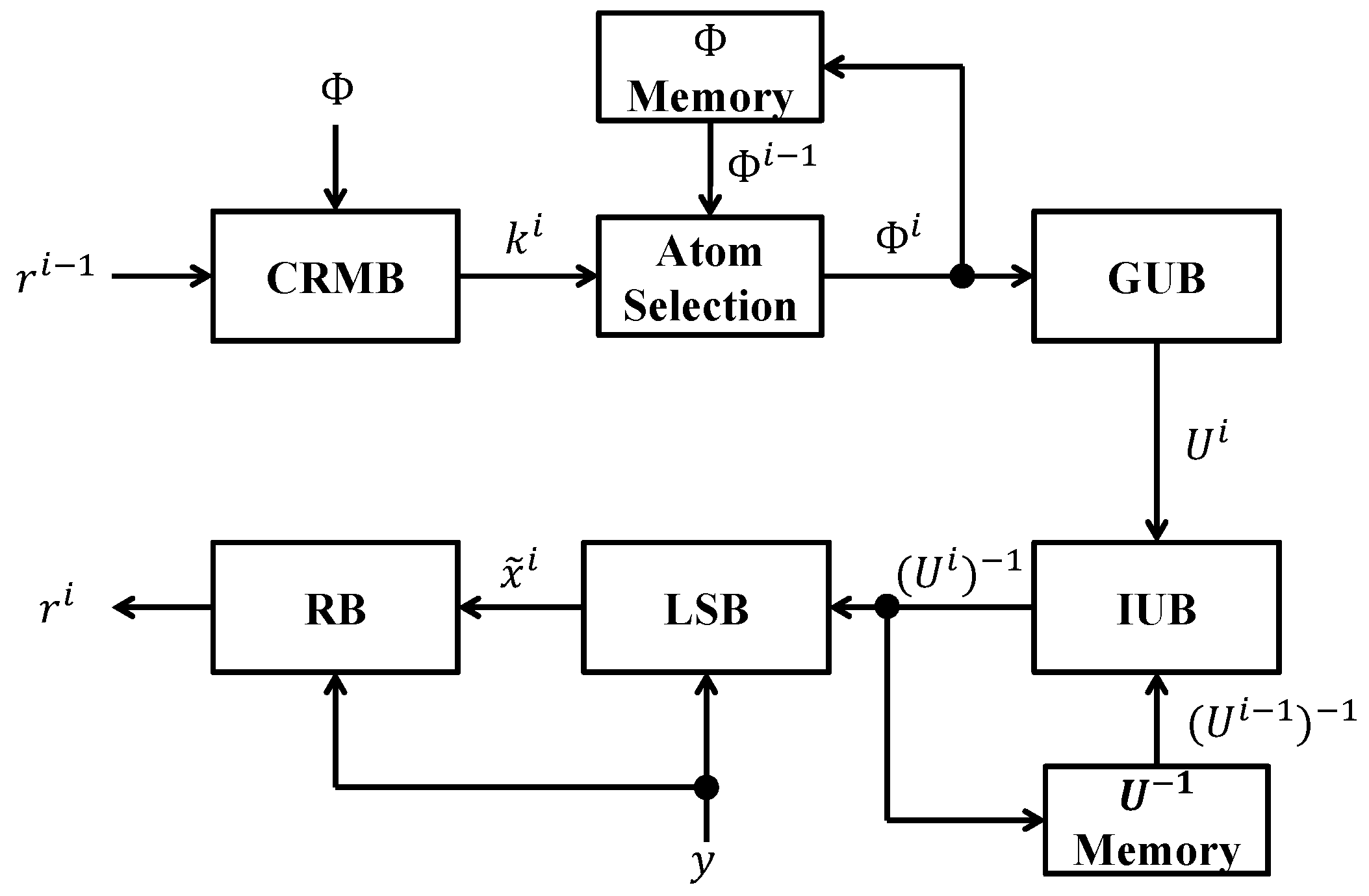
4.5. SOMP Structure with the Proposed Partitioned Inversion
5. Experiment Results
5.1. FPGA Implementation Approach
5.2. Additional Optimisation in FPGA Implementation
5.3. SOMP Hardware Utilization
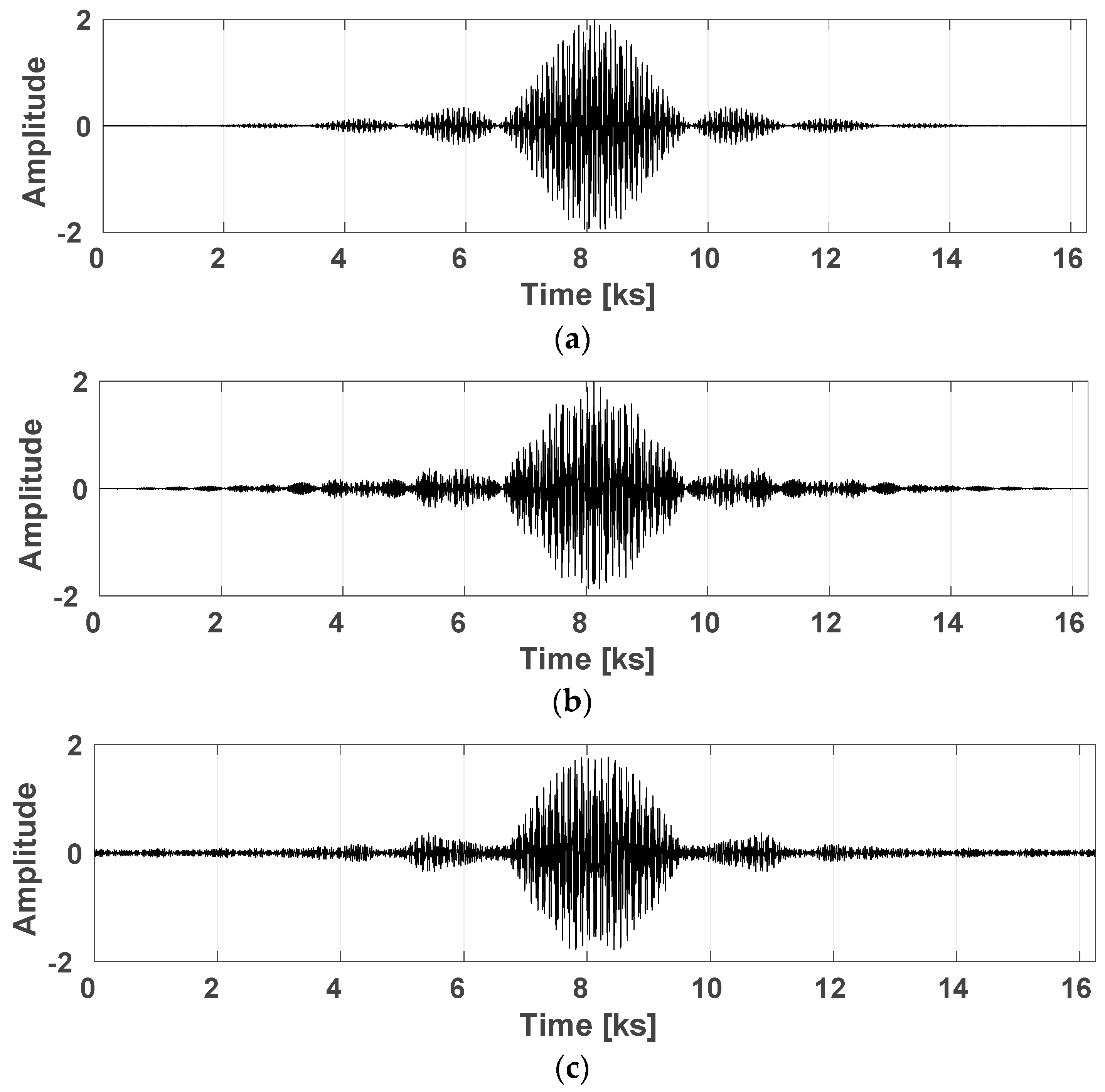
5.4. Signal Reconstruction
5.5. Performance Comparison
6. Conclusions
Author Contributions
Funding
Conflicts of Interest
References
- Candes, E.; Wakin, M. An introduction to compressive sampling. IEEE Signal Process. Mag. 2008, 25, 21–30. [Google Scholar] [CrossRef]
- Pati, Y.; Rezaiifar, R.; Krishnaprasad, P. Orthogonal matching pursuit: Recursive function approximation with applications to wavelet decomposition. In Proceedings of the IEEE Record of The Twenty-Seventh Asilomar Conference on Signals, Systems, and Computers, Pacific Grove, CA, USA, 1–3 November 1993; pp. 40–44. [Google Scholar]
- Tropp, J.; Gilbert, A. Signal recovery from random measurements via orthogonal matching pursuit. IEEE Trans. Inf. Theory 2007, 53, 4655–4666. [Google Scholar] [CrossRef]
- Chen, S.; Donoho, D.; Saunders, M. Atomic decomposition by basis pursuit. SIAM Rev. 2001, 43, 129–159. [Google Scholar] [CrossRef]
- Khan, I.; Singh, M.; Singh, D. Compressive sensing-based sparsity adaptive channel estimation for 5G massive MIMO systems. Appl. Sci. 2018, 8, 2076–3417. [Google Scholar] [CrossRef]
- Sahoo, S.; Makur, A. Signal recovery from random measurements via extended orthogonal matching pursuit. IEEE Trans. Signal Process. 2015, 63, 2572–2581. [Google Scholar] [CrossRef]
- Rabah, H.; Amira, H.; Mohanty, B.; Almaadeed, S.; Meher, P. FPGA implementation of orthogonal matching pursuit for compressive sensing reconstruction. IEEE Trans. Very Large Scale Integr. Syst. 2015, 23, 2209–2220. [Google Scholar] [CrossRef]
- Bai, L.; Maechler, P.; Muehlberghuber, M.; Kaeslin, H. High-speed compressed sensing reconstruction on FPGA using OMP and AMP. In Proceedings of the 19th IEEE International Conference on Electronics, Circuits, and Systems (ICECS), Seville, Spain, 9–12 December 2012; pp. 53–56. [Google Scholar]
- Blache, P.; Rabah, H.; Amira, A. High level prototyping and FPGA implementation of the orthogonal matching pursuit algorithm. In Proceedings of the 11th IEEE International Conference on Information Science, Signal Processing and their Applications (ISSPA), Montreal, QC, Canada, 2–5 July 2012; pp. 1336–1340. [Google Scholar]
- Tropp, J.; Gilbert, A.; Strauss, M. Algorithms for simultaneous sparse approximation. Part 1: Greedy pursuit. Signal Process. 2006, 86, 572–588. [Google Scholar] [CrossRef]
- Determe, J.; Louveaux, J.; Jacques, L.; Horlin, F. On the exact recovery condition of simultaneous orthogonal matching pursuit. IEEE Signal Process. Lett. 2016, 23, 164–168. [Google Scholar] [CrossRef]
- Quan, Y.; Li, Y.; Gao, X.; Xing, M. FPGA implementation of realtime compressive sensing with partial Fourier dictionary. Int. J. Antennas Propag. 2016, 2016, 1671687. [Google Scholar] [CrossRef]
- Septimus, A.; Steinberg, R. Compressive sampling hardware reconstruction. In Proceedings of the IEEE International Symposium on Circuits and Systems (ISCAS), Paris, France, 30 May–2 June 2010; pp. 3316–3319. [Google Scholar]

| Measurement Matrix | Input Matrix |
|---|---|
| Input Matrix | Inversion of Input Matrix |
|---|---|
| Conventional Partitioned Inversion | Proposed Partitioned Inversion |
| Step 1. 2. 3. 4. 5. 6. 7. 8. 9. 10. | Step 1. 2. 3. 4. 5. 6. 7. |
| Inversion | Cholesky-Based [7] | Conventional Partitioned | Proposed Partitioned | |
|---|---|---|---|---|
| Operation | ||||
| Multiplication | ||||
| Add/sub | ||||
| Division | ||||
| Xilinx Kintex UltraScale XCKU115 | Conventional | Proposed |
|---|---|---|
| BRAM | 283 (13.1%) | (14.2%) |
| DSP48E | 2754 (49.9%) | 2032 (36.8%) |
| FF | 225,337 (17%) | 210,577 (15.9%) |
| LUT | 190,742 (28.7%) | 153,447 (23.1%) |
| Sparsity | Clock Frequency | Reconstruction Time | Inversion Type | Data Format | |
|---|---|---|---|---|---|
| Intel Core Duo [7] | 5 | 2.8 GHz | 606 μs | Cholesky-based | 32-bit fixed-point real data |
| FPGA Virtex 7 [12] | 5 | 0.165 GHz | 18.3 μs | QR decomposition-based | 32-bit fixed-point hybrid complex data |
| FPGA Virtex 5 [13] | 5 | 0.039 GHz | 24 μs | Cholesky-based | 32-bit fixed-point real data |
| FPGA Kintex UltraScale [This Work] | 8 | 0.25 GHz | 27 μs | Proposed partitioned inversion | 16- and 32-bit fixed-point complex data |
© 2018 by the authors. Licensee MDPI, Basel, Switzerland. This article is an open access article distributed under the terms and conditions of the Creative Commons Attribution (CC BY) license (http://creativecommons.org/licenses/by/4.0/).
Share and Cite
Kim, S.; Yun, U.; Jang, J.; Seo, G.; Kang, J.; Lee, H.-N.; Lee, M. Reduced Computational Complexity Orthogonal Matching Pursuit Using a Novel Partitioned Inversion Technique for Compressive Sensing. Electronics 2018, 7, 206. https://doi.org/10.3390/electronics7090206
Kim S, Yun U, Jang J, Seo G, Kang J, Lee H-N, Lee M. Reduced Computational Complexity Orthogonal Matching Pursuit Using a Novel Partitioned Inversion Technique for Compressive Sensing. Electronics. 2018; 7(9):206. https://doi.org/10.3390/electronics7090206
Chicago/Turabian StyleKim, Seonggeon, Uihyun Yun, Jaehyuk Jang, Geunsu Seo, Jongjin Kang, Heung-No Lee, and Minjae Lee. 2018. "Reduced Computational Complexity Orthogonal Matching Pursuit Using a Novel Partitioned Inversion Technique for Compressive Sensing" Electronics 7, no. 9: 206. https://doi.org/10.3390/electronics7090206
APA StyleKim, S., Yun, U., Jang, J., Seo, G., Kang, J., Lee, H.-N., & Lee, M. (2018). Reduced Computational Complexity Orthogonal Matching Pursuit Using a Novel Partitioned Inversion Technique for Compressive Sensing. Electronics, 7(9), 206. https://doi.org/10.3390/electronics7090206