Time Sequential Motion-to-Photon Latency Measurement System for Virtual Reality Head-Mounted Displays


Abstract
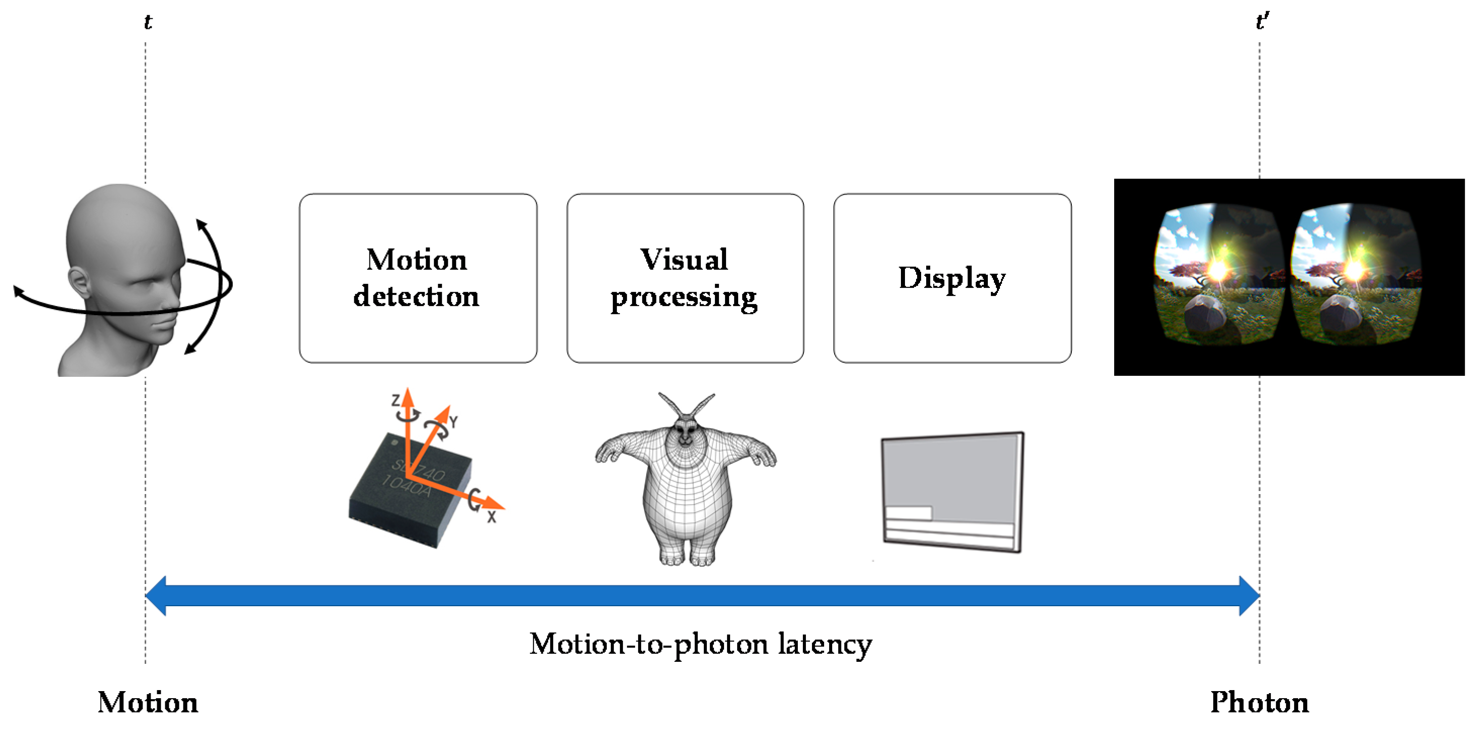
:1. Introduction
2. Proposed Method
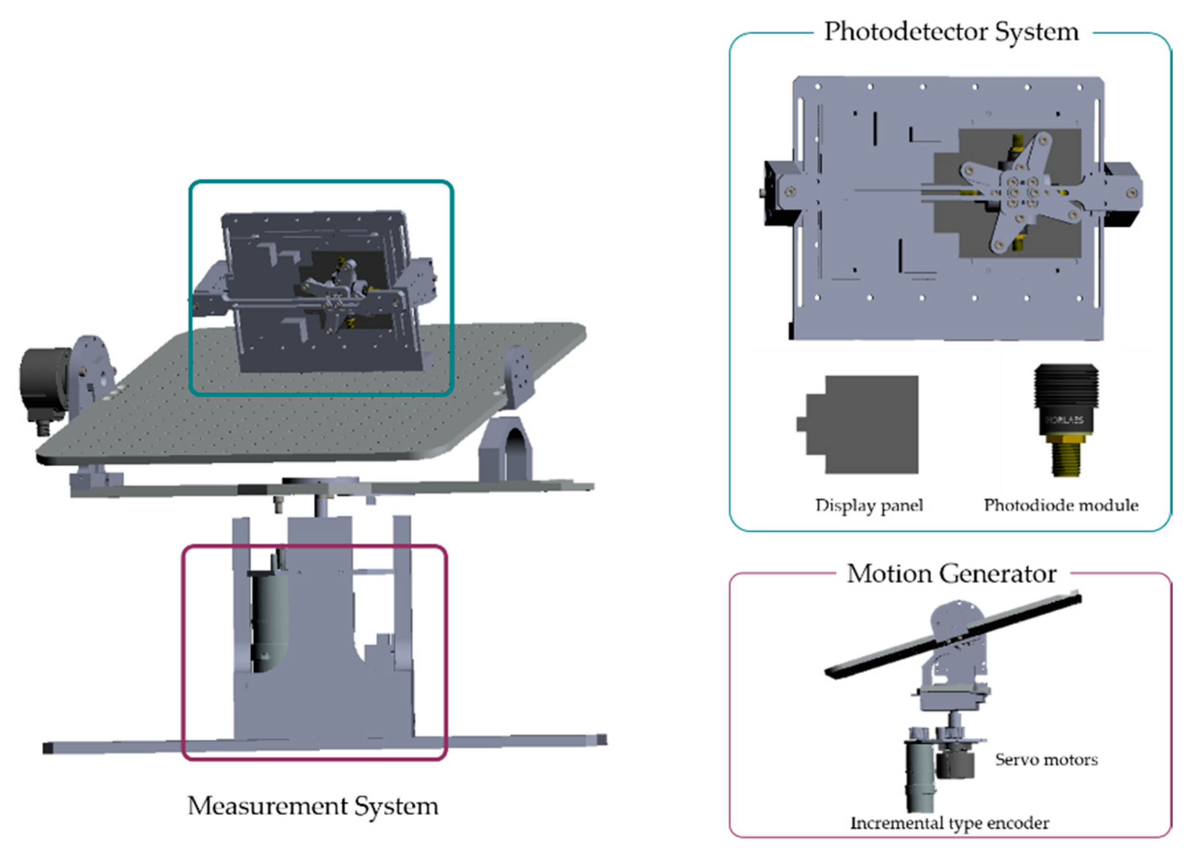
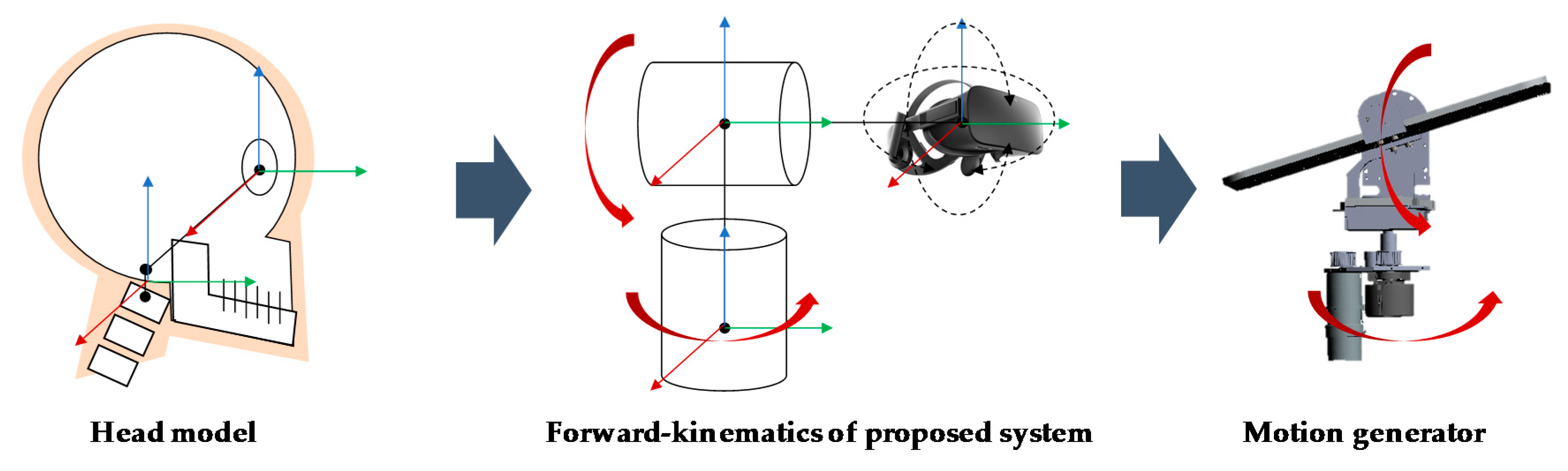
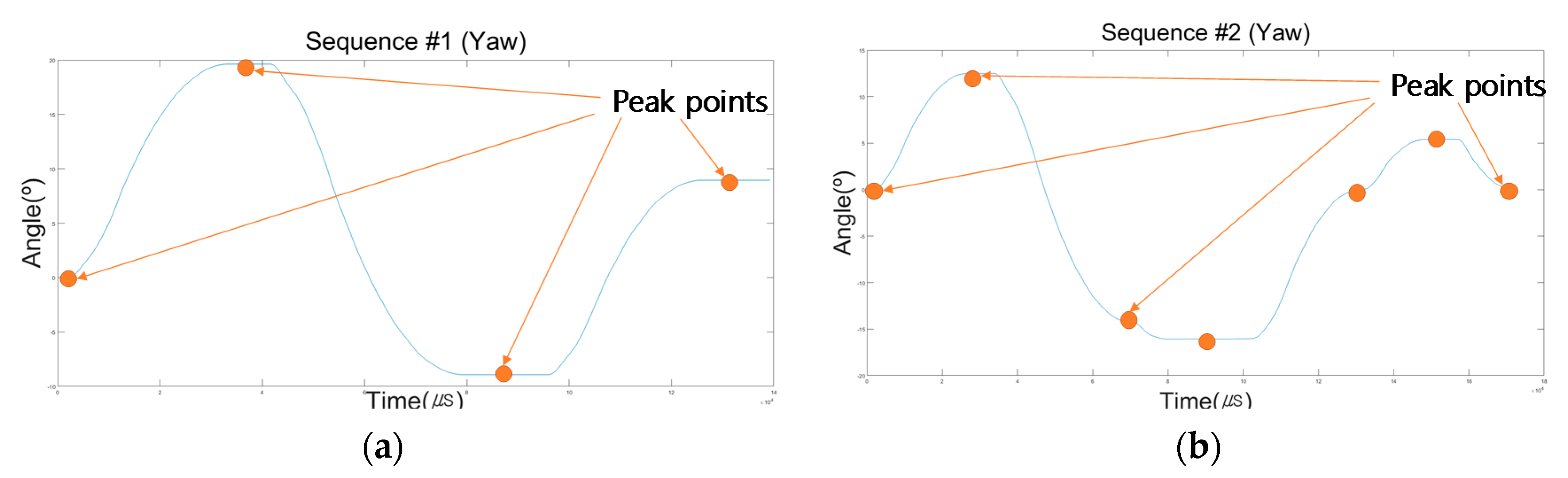
2.1. Motion Generator-Based on Human Neck Movement
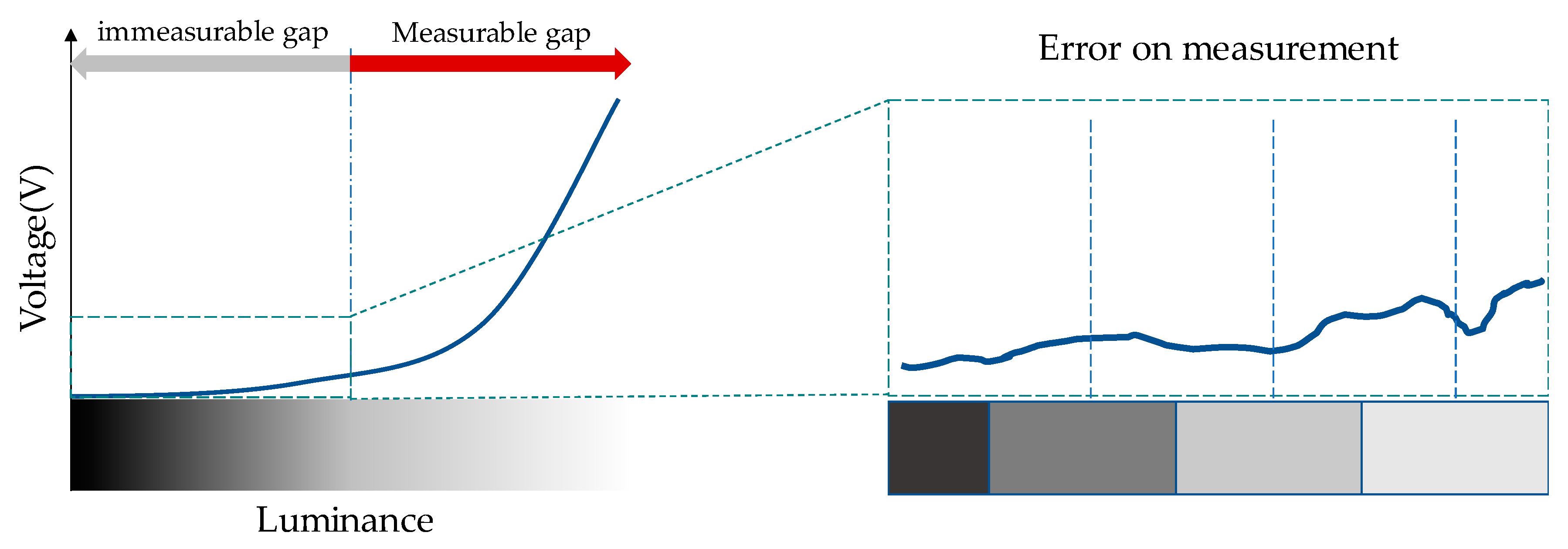
2.2. Measurement Area Design
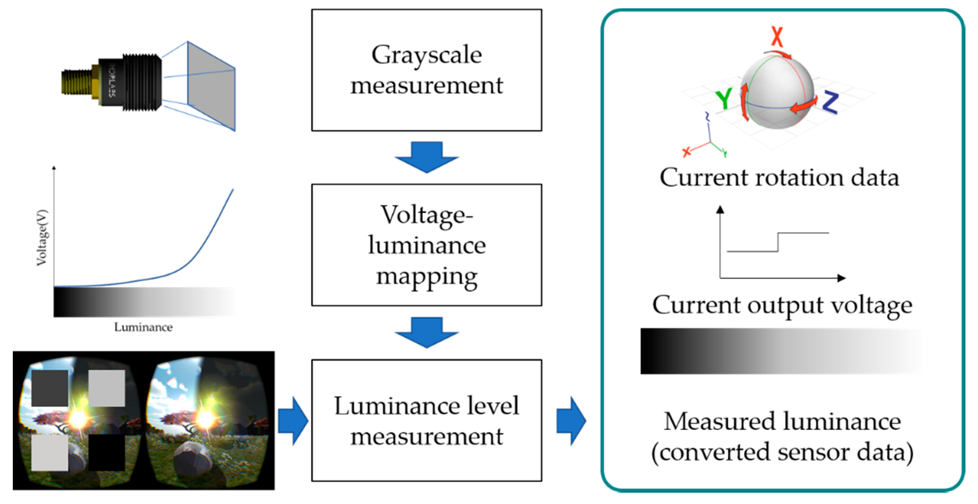
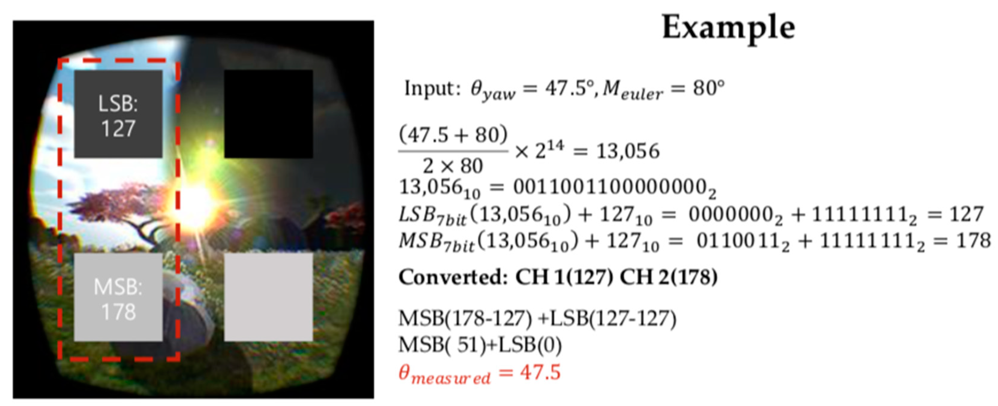
2.3. Voltage Mapping Table
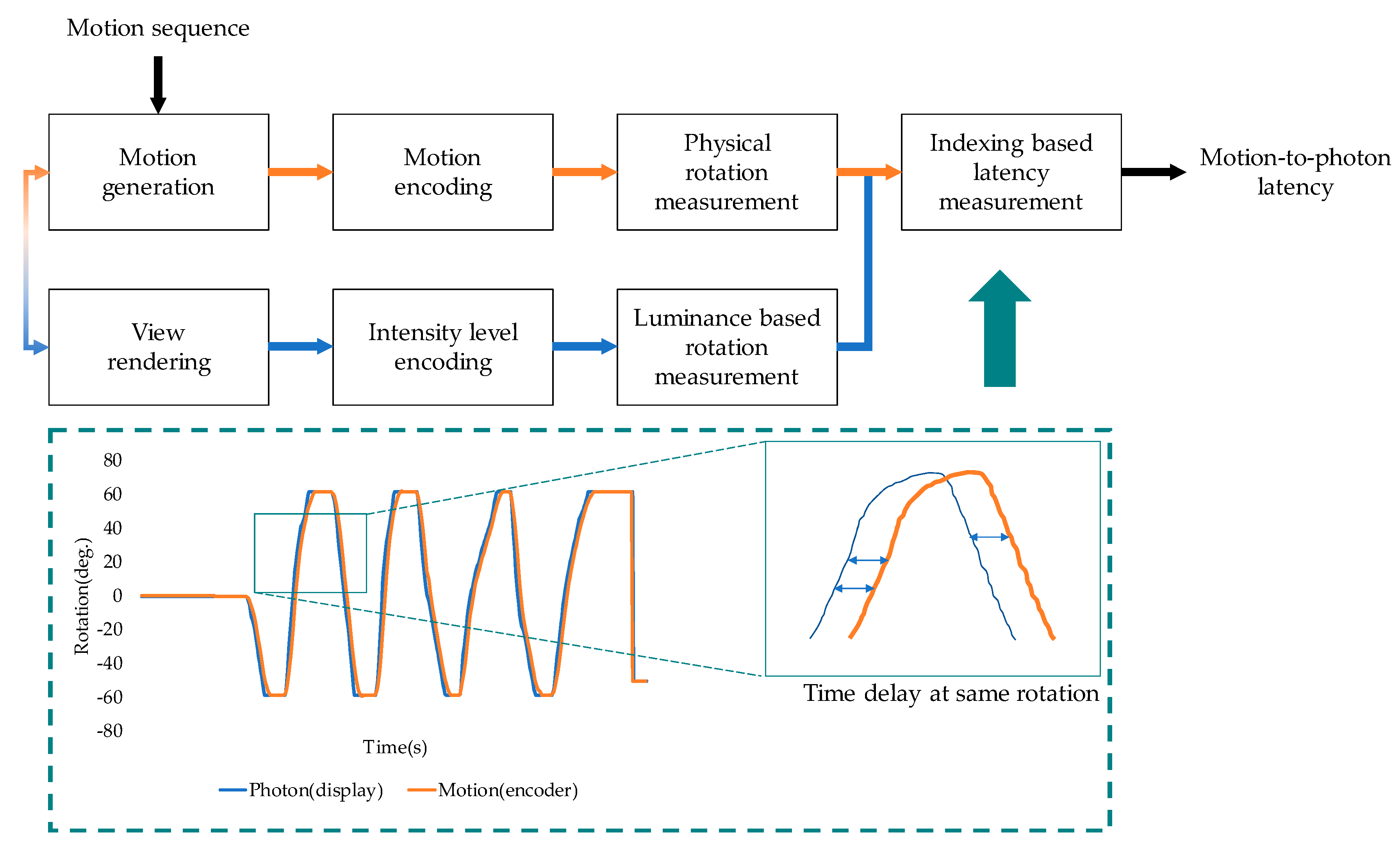
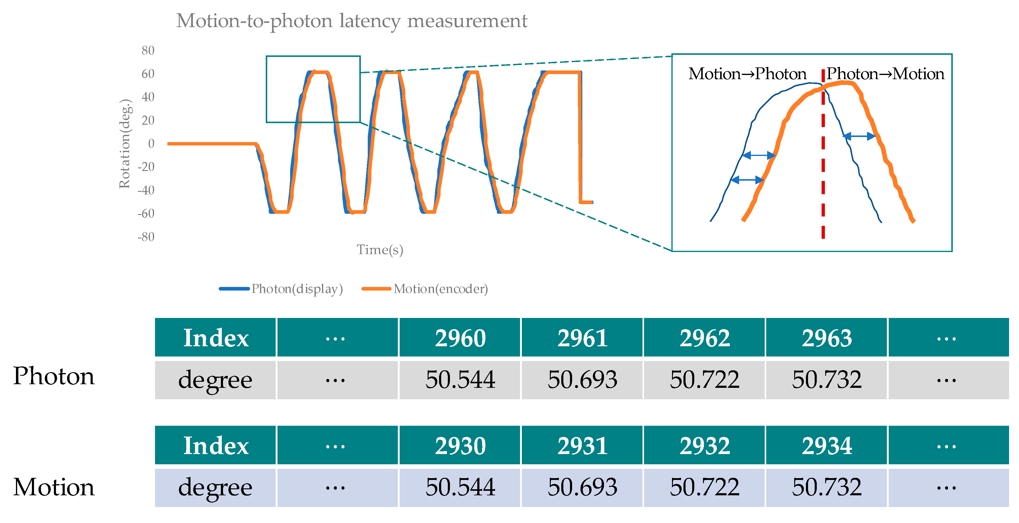
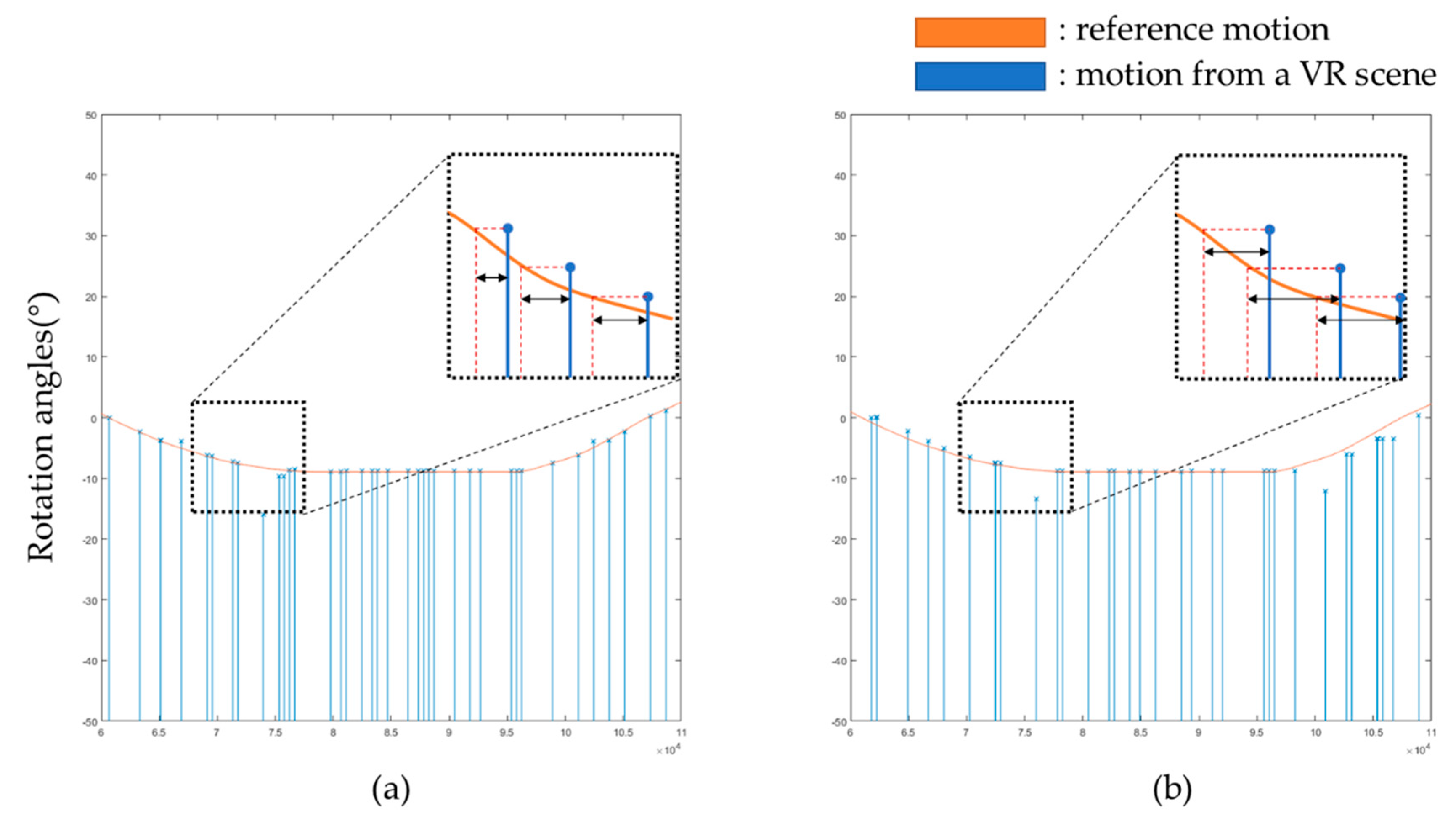
2.4. Measurement of Motion-to-Photon Latency
2.5. Real-Time Measurement and Interface
3. Experimental Results
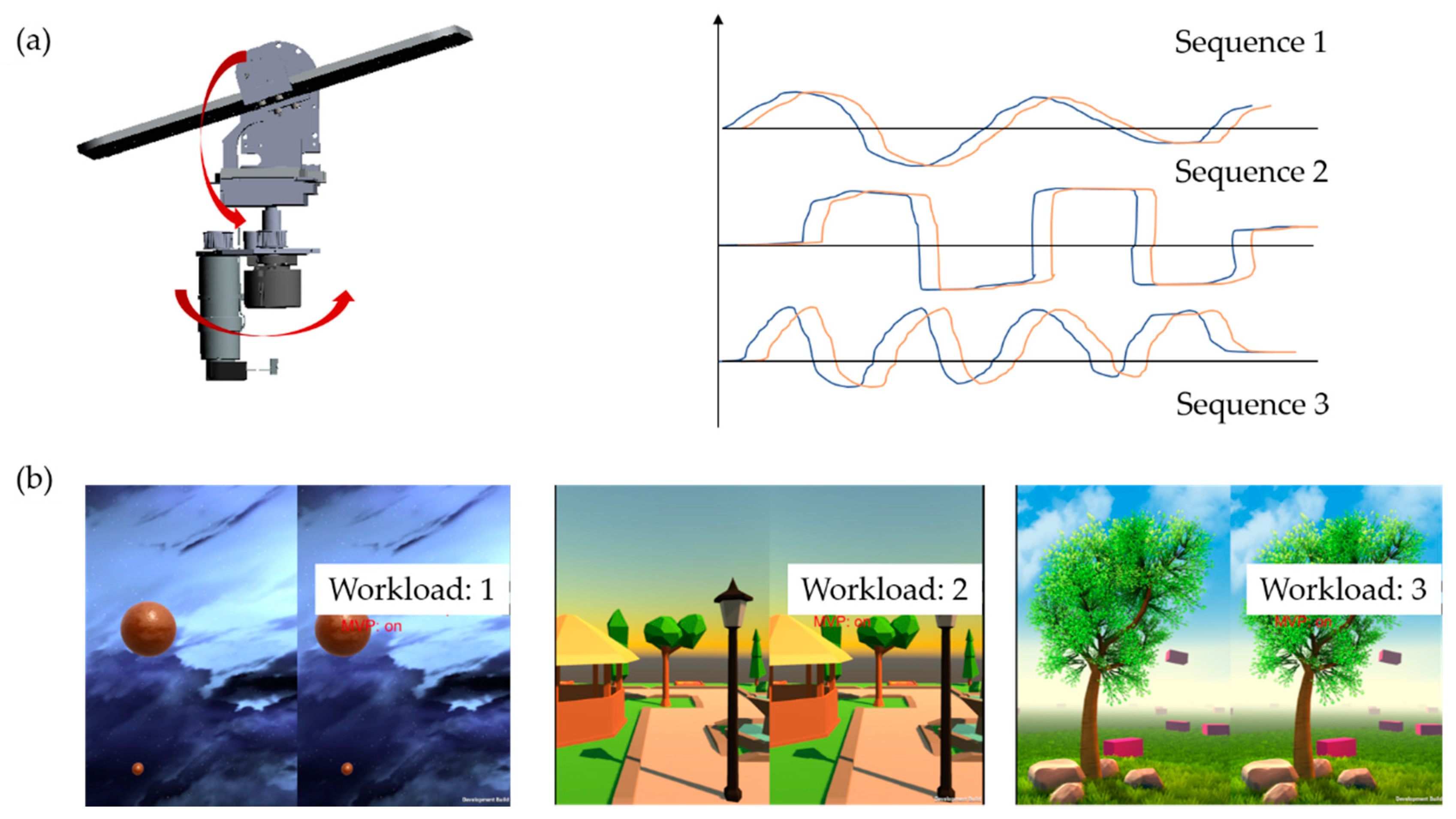
3.1. Position Sequence
3.2. Different Workloads
4. Conclusions
Author Contributions
Acknowledgments
Conflicts of Interest
References
- Chang, S.N.; Chen, W.L. Does visualize industries matter? A technology foresight of global Virtual Reality and Augmented Reality Industry. In Proceedings of the 2017 International Conference on Applied System Innovation (ICASI), Sapporo, Japan, 13–17 May 2017. [Google Scholar]
- Azuma, R.; Baillot, Y.; Behringer, R.; Feiner, S. Recent advances in augmented reality. IEEE Comput. Graph. Appl. 2001, 21, 34–47. [Google Scholar] [CrossRef]
- Iribe, B. Virtual reality—A new frontier in computing. In Proceedings of the AMD Announces 2013 Developer Summit, San Jose, CA, USA, 13 November 2013. [Google Scholar]
- Justin, M.; Diedrick, M.; Stoffregen, T. The virtual reality head-mounted display Oculus Rift induces motion sickness and is sexist in its effects. Exp. Brain Res. 2017, 3, 889–901. [Google Scholar]
- LaValle, S.M.; Yershova, A.; Katsev, M.; Antonov, M. Head tracking for the Oculus Rift. In Proceedings of the 2014 IEEE International Conference on Robotics and Automation (ICRA), Hong Kong, China, 31 May–7 June 2014. [Google Scholar]
- Evangelakos, D.; Mara, M. Extended TimeWarp latency compensation for virtual reality. In Proceedings of the 20th ACM SIGGRAPH Symposium on Interactive 3D Graphics and Games, Redmond, WA, USA, 27–28 February 2016. [Google Scholar]
- Tsai, Y.J.; Wang, Y.X.; Ouhyoung, M. Affordable system for measuring motion-to-photon latency of virtual reality in mobile devices. In Proceedings of the SIGGRAPH Asia 2017 Posters, Bangkok, Thailand, 27–30 November 2017. [Google Scholar]
- Lincoln, P.; Blate, A.; Singh, M.; Whitted, T.; State, A.; Lastra, A.; Fuchs, H. From motion to photons in 80 microseconds: Towards minimal latency for virtual and augmented reality. IEEE Trans. Visual Comput. Graph. 2016, 22, 1367–1376. [Google Scholar] [CrossRef] [PubMed]
- Seo, M.; Choi, S.; Lee, S.; Lee, E.; Baek, J.; Kang, S. Photosensor-based latency measurement system for head-mounted displays. Sensors 2017, 17, 1112. [Google Scholar] [CrossRef] [PubMed]
- Sharkey, M.; Murray, W.; Heuring, J. On the kinematics of robot heads. IEEE Trans. Rob. Autom. 1997, 13, 437–442. [Google Scholar] [CrossRef]
- Funda, J.; Taylor, H.; Paul, P. On homogeneous transforms, quaternions, and computational efficiency. IEEE Trans. Rob. Autom. 1990, 6, 382–388. [Google Scholar]
- Denavit, J.; Hartenberg, S. A kinematic notation for lower-pair mechanisms based on matrices. J. Appl. Mech. 1955, 1, 215–221. [Google Scholar]
- Kim, J.; Kumar, R. Kinematics of robot manipulators via line transformations. J. Rob. Syst. 1990, 7, 649–674. [Google Scholar] [CrossRef]
- Kucuk, S.; Bingul, Z. Robot kinematics: Forward and inverse kinematics. In Industrial Robotics: Theory, Modelling and Control; INTECH Open: London, UK, 2006. [Google Scholar]
- Eberly, D.H. 3D Game Engine Design: A Practical Approach to Real-Time Computer Graphics; CRC Press: Boca Raton, FL, USA, 2006. [Google Scholar]
- Jack, K.; Tsatsulin, V. Dictionary of Video and Television Technology; Gulf Professional Publishing: Houston, TX, USA, 2002. [Google Scholar]
- Kariya, T.; Kurata, H. Generalized least squares estimators. In Generalized Least Squares, 1st ed.; John Wiley & Sons: Hoboken, NJ, USA, 2004; pp. 25–67. [Google Scholar]
- Oculus Rift DK 2 Overview of the DK2 and SDK 0.4. Available online: https://developer.oculus.com/documentation/pcsdk/0.4/concepts/dg-intro-version/ (accessed on 2 September 2017).
- Maxon RE 40 40 mm, Graphite Brushes, 150 Watt Specifications. Available online: https://www.maxonmotor.com/medias/sys_master/root/8825409404958/17-EN-132.pdf (accessed on 2 September 2017).
- EPOS2 50/5, Digital Positioning Controller, 5 A, 11 - 50 VDC Specifications. Available online: https://www.maxonmotor.com/medias/sys_master/root/8821075705886/16-421-422-423-425-EN.pdf (accessed on 2 September 2017).
- EIL580 Mounted Optical Incremental Encoders Specification. Available online: http://www.baumer.com/es-en/products/rotary-encoders-angle-measurement/incremental-encoders/58-mm-design/eil580-standard (accessed on 2 September 2017).
- SM05PD Mounted Photodiodes – SM05 and SM1 Compatible Specifications. Available online: https://www.thorlabs.com/Images/PDF/Vol18_773.pdf (accessed on 2 September 2017).
- PicoScope 4824 Data Sheet. Available online: https://www.picotech.com/legacy-document/datasheets/PicoScope4824.en-2.pdf (accessed on 2 September 2017).
- Intel Core i7-6700K Processor Specifications. Available online: https://ark.intel.com/products/88195/Intel-Core-i7-6700K-Processor-8M-Cache-up-to-4_20-GHz (accessed on 2 September 2017).
- Geforce GTX 1080 Graphic card Specifications. Available online: https://www.nvidia.com/en-us/geforce/products/10series/geforce-gtx-1080/ (accessed on 2 September 2017).


| Orientation | Yaw | Pitch | |||
|---|---|---|---|---|---|
| Number of Sequences | 1 | 2 | 1 | 2 | |
| Peak point | 1 | 0.00 | 0.00 | 0.00 | 0.00 |
| 2 | 19.10 | 13.50 | −14.00 | 19.10 | |
| 3 | 5.10 | −14.20 | −5.00 | 5.10 | |
| 4 | 0.00 | −15.00 | 13.50 | 0.00 | |
| 5 | −8.90 | 5.00 | 6.50 | −8.90 | |
| 6 | 0.00 | 0.00 | 0.00 | 0.00 | |
| Orientation | Yaw | Pitch | ||
|---|---|---|---|---|
| Number of Sequences | 1 | 2 | 1 | 2 |
| Min. (ms) | 21.83 | 15.78 | 23.42 | 32.10 |
| Max. (ms) | 63.72 | 69.33 | 53.75 | 65.36 |
| Average (ms) | 46.55 | 47.42 | 43.87 | 49.45 |
| Rendering Workload | 0 | 1 | 2 | 3 |
|---|---|---|---|---|
| Number of objects | 2 | 7 | 12 | 17 |
| Vertices | 0.8 M | 2.4 M | 4.8 M | 9.5 M |
| Rendering Workload | 0 | 1 | 2 | 3 |
|---|---|---|---|---|
| Min. (ms) | 21.80 | 45.30 | 88.30 | 120.15 |
| Max. (ms) | 63.75 | 89.75 | 133.65 | 198.24 |
| Average (ms) | 46.55 | 63.22 | 101.29 | 154.63 |
© 2018 by the authors. Licensee MDPI, Basel, Switzerland. This article is an open access article distributed under the terms and conditions of the Creative Commons Attribution (CC BY) license (http://creativecommons.org/licenses/by/4.0/).
Share and Cite
Choi, S.-W.; Lee, S.; Seo, M.-W.; Kang, S.-J. Time Sequential Motion-to-Photon Latency Measurement System for Virtual Reality Head-Mounted Displays. Electronics 2018, 7, 171. https://doi.org/10.3390/electronics7090171
Choi S-W, Lee S, Seo M-W, Kang S-J. Time Sequential Motion-to-Photon Latency Measurement System for Virtual Reality Head-Mounted Displays. Electronics. 2018; 7(9):171. https://doi.org/10.3390/electronics7090171
Chicago/Turabian StyleChoi, Song-Woo, Siyeong Lee, Min-Woo Seo, and Suk-Ju Kang. 2018. "Time Sequential Motion-to-Photon Latency Measurement System for Virtual Reality Head-Mounted Displays" Electronics 7, no. 9: 171. https://doi.org/10.3390/electronics7090171
APA StyleChoi, S.-W., Lee, S., Seo, M.-W., & Kang, S.-J. (2018). Time Sequential Motion-to-Photon Latency Measurement System for Virtual Reality Head-Mounted Displays. Electronics, 7(9), 171. https://doi.org/10.3390/electronics7090171