Enabling Off-Road Autonomous Navigation-Simulation of LIDAR in Dense Vegetation

Abstract

Machine learning techniques have accelerated the development of autonomous navigation algorithms in recent years, especially algorithms for on-road autonomous navigation. However, off-road navigation in unstructured environments continues to challenge autonomous ground vehicles. Many off-road navigation systems rely on LIDAR to sense and classify the environment, but LIDAR sensors often fail to distinguish navigable vegetation from non-navigable solid obstacles. While other areas of autonomy have benefited from the use of simulation, there has not been a real-time LIDAR simulator that accounted for LIDAR–vegetation interaction. In this work, we outline the development of a real-time, physics-based LIDAR simulator for densely vegetated environments that can be used in the development of LIDAR processing algorithms for off-road autonomous navigation. We present a multi-step qualitative validation of the simulator, which includes the development of an improved statistical model for the range distribution of LIDAR returns in grass. As a demonstration of the simulator’s capability, we show an example of the simulator being used to evaluate autonomous navigation through vegetation. The results demonstrate the potential for using the simulation in the development and testing of algorithms for autonomous off-road navigation.

1. Introduction

Laser ranging sensors, commonly referred to as LIDAR, are ubiquitous in off-road autonomous navigation because they provide a direct measurement of the geometry of the operating environment of the robot [1]. One of the ongoing issues with LIDAR perception is the inability of the sensor to distinguish between navigable obstacles like grass and non-navigable solid obstacles. This problem is stated clearly by [2]:

Among the more pervasive and demanding requirements for operations in vegetation is the discrimination of terrain from vegetation-of rocks from bushes... Failure to make the distinction leads to frustrating behaviors including unnecessary detours (of a timid system) around benign vegetation or collisions (of an aggressive system) with rocks misclassified as vegetation.

While there has been progress over the last decade in addressing the perception issues associated with LIDAR [3,4], the mitigating techniques have primarily been developed and refined experimentally. Recent advances in simulation for robotics have demonstrated that autonomy algorithms can be developed and tested in simulation [5,6,7]. However, up until now simulations have either lacked the fidelity to realistically capture LIDAR-vegetation interaction or been computationally slow and difficult to integrate with existing autonomy algorithms [8].

In this work, the development, validation, and demonstration of a realistic LIDAR simulator that can be used to develop and test LIDAR processing algorithms for autonomous ground vehicles is presented. It accurately captures the interaction between LIDAR and vegetation while still maintaining real-time performance. Real-time performance is maintained by making some simplifying approximations and by using Embree, an open-source ray-tracing engine from Intel [9], for ray-tracing calculations, making the simulator useful for integration into “in-the-loop” simulations of autonomous systems.

LIDAR Basics

While there are several different types of LIDAR sensors, this paper focuses on incoherent micro-pulse LIDAR sensors, commonly referred to as Time-of-Flight (TOF) sensors, as this type of LIDAR is by far the most common type used in outdoor autonomous navigation. The operating principle of TOF LIDAR is to measure the time between the initial pulse of the LIDAR and the arrival of the reflected pulse, and divide this time by the speed of light to derive a distance [10].

Most LIDAR sensors used in autonomous navigation also feature a rotating scanning mechanism that allows the laser to sample multiple locations. For example, the SICK sensor scans by having a stationary laser reflect from a rotating mirror, producing a planar “slice” of the environment, while the Velodyne sensors feature an array of 16, 32, or 64 laser-sensor pairs in a rotating housing, producing a 3D point cloud with each full rotation of the sensor.

There are several different sources of error in LIDAR range measurements. The finite duration of the laser pulse, discretization of the reflected signal for processing, and atmospheric scattering properties all contribute to the error. However, this work focuses on the divergence of the laser beam and how the diverging beam’s interaction with the fine scale detail of vegetation results in error in the LIDAR range measurement.

In the following sections, the paper briefly outlines the materials and methods of the simulated experiments (Section 2), describes the results of simulations (Section 3) and presents discussion and conclusions based on these results (Section 4 and Section 5).

2. Materials and Methods

This work describes the development of a high-fidelity, physics-based LIDAR simulator for off-road autonomous vehicles. The method of validation of the simulator is qualitative comparison to previously published experiments on LIDAR interaction with vegetation and other extended objects.

The LIDAR simulation has several key objectives that guided development decisions. First, it must simulate common robotic LIDAR sensors such as the Velodyne HDL-64E operating in highly-vegetated outdoor environments in real-time. Second, it must realistically capture the salient characteristics of laser-beam interaction with blades of grass and leaves. Third, the simulation must be generic enough to simulate a variety of different LIDAR sensors with only the parameters obtained from specification sheets and other freely available data. With these requirements in mind, it is noted that the LIDAR simulator presented here was not developed to support the design and development of LIDAR sensors. Rather, the simulator was developed to be used in robotics applications where real-time LIDAR simulation is a requirement.

2.1. Software

The simulator is written in C++ with MPI bindings. The compiler used was the Intel C++ compiler. Third party libraries used in the development of the simulator are given in

Table 1. Third-party software libraries used by the simulator.

Software	Available at
Cimg	cimg.eu
TinyObjLoader	https://github.com/syoyo/tinyobjloader
OpenGL Mathematics (GLM)	https://github.com/g-truc/glm
Rapidjson	https://github.com/Tencent/rapidjson
HosekWilkie Sky Model	http://cgg.mff.cuni.cz/projects/SkylightModelling/
Rinex	https://www.ngs.noaa.gov/gps-toolbox/rinex.htm
a-star	https://github.com/hjweide/a-star
Embree	https://github.com/embree

.

2.2. Hardware

Two different computers were used for the simulations in this work. The LMS-291 simulations were run on a Linux workstation using four Intel Xeon E5 2.9 GHz CPUs. The Velodyne simulations were run with 40 Intel Ivy Bridge processors on Mississippi State University’s High Performance Computer, Shadow [11].

3. Results

This section describes the results of simulated LIDAR experiments and their comparison to previously published data. This section also outlines the development of an analytical range model for LIDAR penetration into grass for comparison to simulated results.

3.1. Simulation Parameters

The parameters used by the LIDAR model are listed in

Table 2. LIDAR simulation parameters.

Parameter	Units	HDL-32E
Min & max horizontal angle	degrees	[−180, 180]
Horizontal resolution	degrees	0.16
Min & max vertical angle	degrees	[−30.6623, 10.67]
Vertical resolution	degrees	1.3333
Min range	m	1.0
Max range	m	70
Beam spot shape	circular, rectangular, or elliptical	rectangular
Horizontal divergence	rad	0.0033
Vertical divergence	rad	0.0007
Signal cutoff	m	1.0
Mode	first, last, strongest, strongest & last	strongest or last

, all of which are typically found in sensor specification sheets. As an illustrative example, the parameters used in the simulation for a common LIDAR sensor, the Velodyne HDL-32E [12], are also listed.

3.2. Physics of Laser-Vegetation Interaction

There are three processes which need to be simulated in order to realistically capture the salient characteristics of the laser-beam interaction with vegetation. First, the divergence and shape of the laser beam should be taken into account. Second, the scattering properties of the leaves and vegetation in the environment must be simulated. Finally, the on-board processing of the LIDAR sensor also influences the result.

3.2.1. Beam Divergence

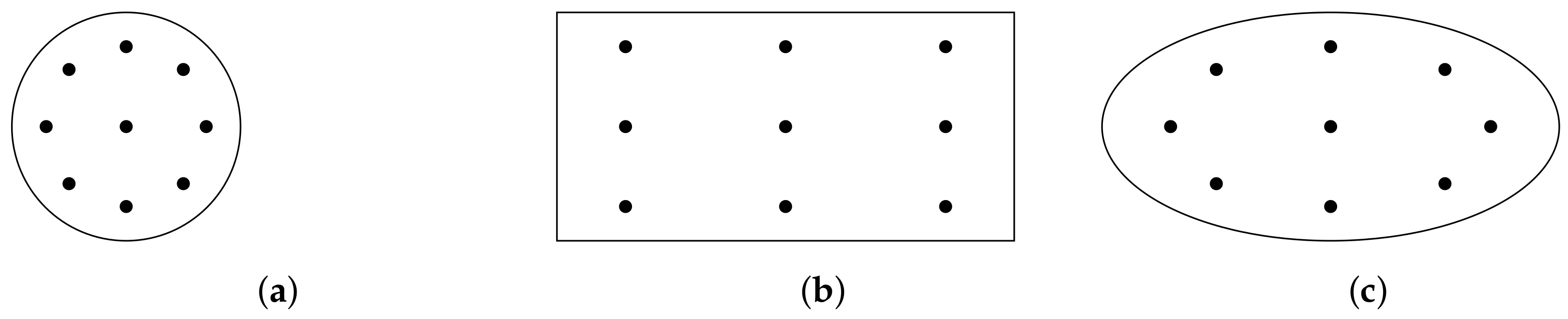
In order to simulate beam divergence, the simulator uses the Embree ray-tracing kernel [9,13] to over-sample each laser pulse and estimate a return signal. The signal pulse is then processed according to the specified mode of the LIDAR, which can be first, strongest, or last return, or both strongest and last. Ideally, each beam would be randomly sampled to build up a representative reflected pulse. However, in order to maintain the real-time requirement, the simulator uses a fixed 9-point stencil for each of the three beam spot shapes. The three stencils are shown in Figure 1a–c.

In the simulation, nine rays are traced from the sensor origin through the stencil points for each beam pulse. The location of the stencil points is defined by the divergence values specified for the sensor at 1 m of range. For example, for a sensor located at the origin, oriented with the z-axis up, having a circular beam spot with divergence $\gamma$ and beam oriented along the x-axis, the stencil points would lie in a circle in the $y-z$ plane with radius given by

$$\mathtt{radius}=\sqrt{(}2)tan(\gamma /2)/4$$

and centered around the x-axis at $x=1$.

3.2.2. Scattering from Leaves and Vegetation

The environment is modeled as a collection of triangular meshes, with each triangle attributed with a reflectance value. All materials in the scene are assumed to be diffuse reflectors, so if a ray intersects a triangle, the intensity of the retro-reflected ray is given by

$$I=\rho I_{0}cos\left(\theta \right)$$

(1)

where $\rho$ is the surface reflectance (with possible values ranging from 0 to 1), $\theta$ is the angle between the surface normal and the ray, and $I_0$ is the intensity of the laser. In the simulator, $I_0=1$ for all sensors and perform all calculations in relative intensity. Multiply scattered rays are not considered in the simulation. Although multiply-scattered rays can introduce anomalies in environments with highly reflective materials, natural materials tend to reflect diffusely with values of $\rho <0.5$, in which case the intensity of multiply scattered rays typically falls below the detection threshold of the receiver.

3.2.3. Signal Processing

For each pulse, all reflected rays are stored in a reflected signal. The range is then extracted from the signal according to the mode of the LIDAR. If the mode is “strongest”, the ray with the most intense reflection is used to calculate the distance. If the mode is “last”, the ray with the furthest distance (and longest time) is returned. It is also possible to return both the strongest and last signals. Finally, if the mode is set to “first”, all signals between the closest reflection (in time and distance) and those within the “signal cutoff” distance of the closest return are averaged. The signal cutoff parameter accounts for the fact that LIDAR sensors typically do not average over the time window of the entire pulse. The value of the signal cutoff parameter can be inferred from laboratory measurements [14]. Figure 2 illustrates how the signal cutoff parameter is used to process the signals in the simulation.

3.3. Real-Time Implementation

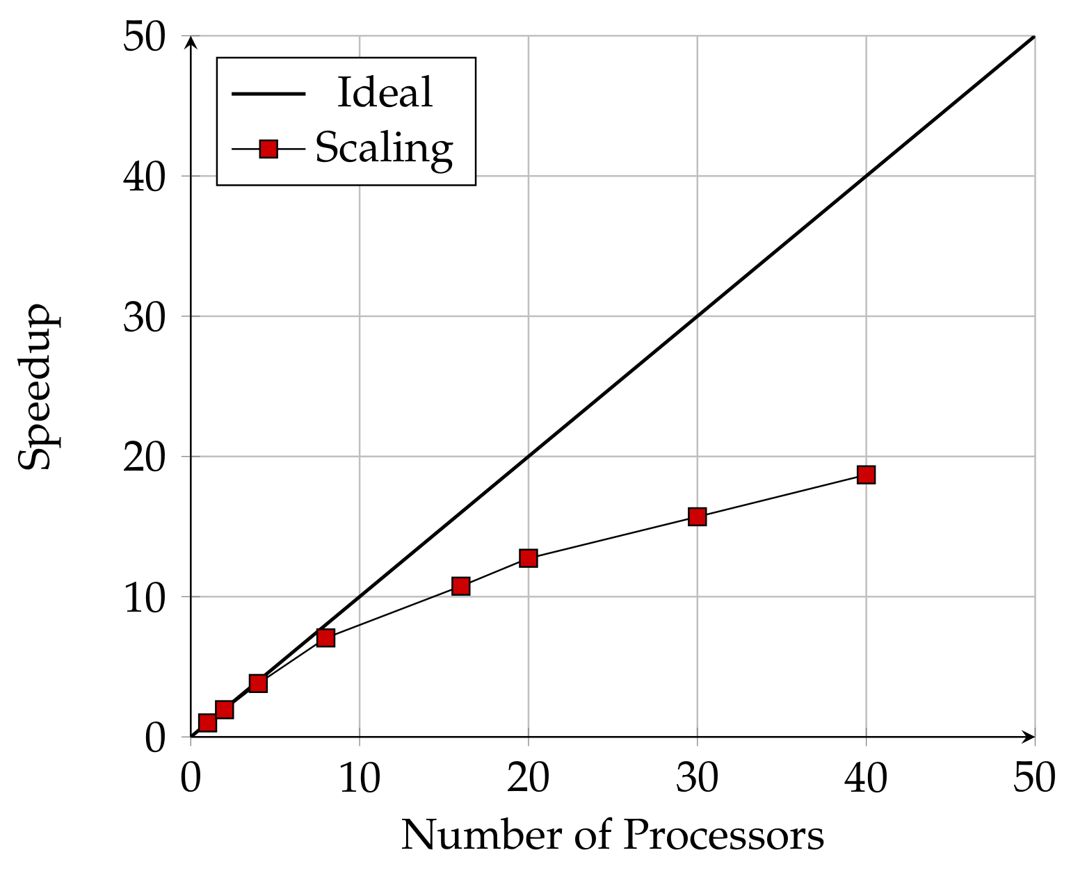
In the example simulations shown in the following sections, the simulated environment contains over 193 million triangles. A sensor like the Velodyne HDL-64E returns about 10${}^6$ points per second, and the simulator traces 9 rays per pulse. This means that the simulation must perform $\mathcal{O}\left({10}^{15}\right)$ ray-triangle intersections per second of simulation time. Even with a ray-tracing kernel like Embree that uses bounding-volume hierarchy acceleration, ray-tracing simulations on this scale require additional parallelization in order to maintain real-time speed.

The Message Passing Interface (MPI) [15] is used to parallelize each scan by laser pulse so that each bundle of 9 rays can be simulated independently. This method is embarrassingly parallel and scales well with the addition of processors. Figure 3 shows the scaling of the code with the number of processors used.

The Sick LMS-291 and the Velodyne HDL-64E were used for computational performance bench-marking. The LMS-291 simulation was run on 4 processors at approximately 30% faster than real time (6.8 s of simulated time in 4.7 s of wall time). The HDL-64E was run on 40 processors at approximately 30% faster than real time (6.8 s of simulated time in 4.7 s of wall time). Details about the hardware used to run the simulations are given in Section 2.2. These examples demonstrate that the implementation is capable of achieving real-time performance, even for very complex LIDAR sensors and environment geometries.

3.4. Simulation Validation

The requirements for validation of physics-based simulation can vary in rigor depending on the application. Accuracy requirements must be defined by the user, and this creates well-known difficulties when generating synthetic sensor data for autonomous vehicle simulations [16]. In the sections above, the development of a generalized LIDAR simulation that captures the interaction between LIDAR and vegetation was presented. The simulation is not optimized for a particular model of LIDAR sensor or type of environment. Therefore, in order to validate the simulation, is of primary importance to qualitatively reproducing well-known LIDAR-vegetation interaction phenomenon. To this end, three validation cases are presented. In the first case, the results of the simulation are compared to an analytical model. Next, simulation results are compared to previously published laboratory experiments. Finally, the simulation is compared to previously published controlled field experiments. All three cases show good qualitative agreement of the simulation with the expected results.

3.4.1. Comparison to Analytical Model

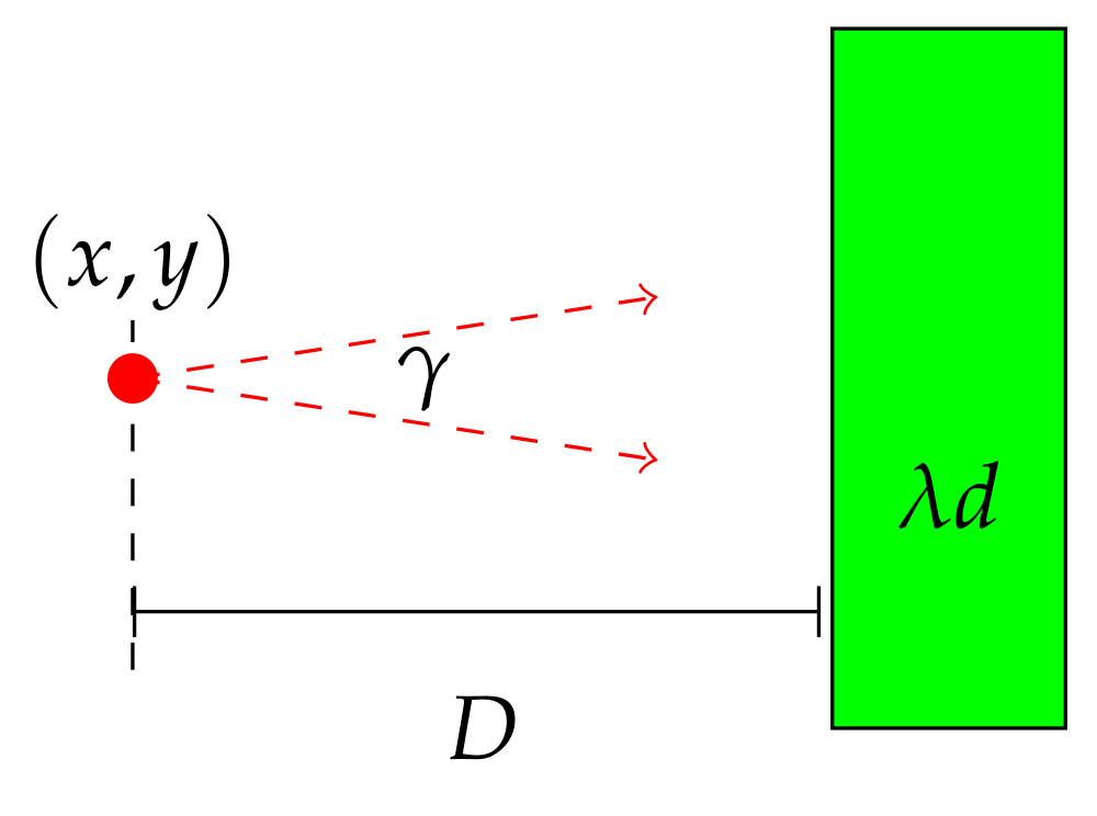
The statistics of LIDAR range returns in grass have been studied for nearly two decades. In particular, Macedo, Manduchi, and Matthies [3] presented an analytical model for the range distribution of LIDAR returns in grass that was based on the exponential distribution function, and this model has been cited frequently in subsequent works [4,14,17,18]. Accounting for the beam divergence, Ref. [3] present the following model for the probability distribution of the LIDAR interacting with a stand of grass, modeled as randomly placed, uniform diameter cylinders.

$$p\left(r\right)=\lambda d(1+ar)e^{-\lambda d(r-D)(1+a{(r+D)}^2/2)}U(r-D)$$

(2)

where $\lambda$ is the number density of the grass per square meter, d is the average grass stem diameter (meters), D is the distance between the laser and the edge of the grass-stand (meters), r is the measured range (meters), and a is related to the laser beam divergence, $\gamma$ (radians) by

$$a=2tan(\gamma /2)$$

(3)

Although the details of the derivation of Equation (2) are not presented in [3], it appears that the model was developed by assuming that the LIDAR’s returned distance would be the nearest distance encountered along the beam spot profile. However, the exponential model has the unsatisfactory result that the most likely returned distance is D, which runs counter to simple geometrical considerations. Additionally, as noted in [3], TOF LIDAR sensors will measure an average over the spatial resolution of the beam spot. The exponential model does not properly account for this averaging over the entire width of the returned pulse. Therefore, an improved analytical model is needed.

Noting that the distribution of the average of multiple samples of an exponentially distributed random variable is a gamma distribution, an improved analytical model based on the gamma distribution is proposed. In the case of a laser beam, the integration is continuous over the width of the beam. Noting that the beam spot factor is proportional to $a{D}^2\approx \gamma D^2$ for small values of $\gamma$ [3], the continuous variable of integration is

$$\alpha =1+\gamma D^2.$$

(4)

The range probability equation is then given by the gamma distribution

$$p\left(r\right)=\frac{{(r-D)}^{\alpha -1}{\left(\alpha \lambda d\right)}^{\alpha }}{\Gamma \left(\alpha \right)}{e}^{-\alpha \lambda d(r-D)}$$

(5)

where $\Gamma$ is the gamma function. This choice of $\alpha$ gives the desirable property that when the divergence is zero, the model reproduces the exponential model while tending towards a normal distribution as $\alpha$ gets large.

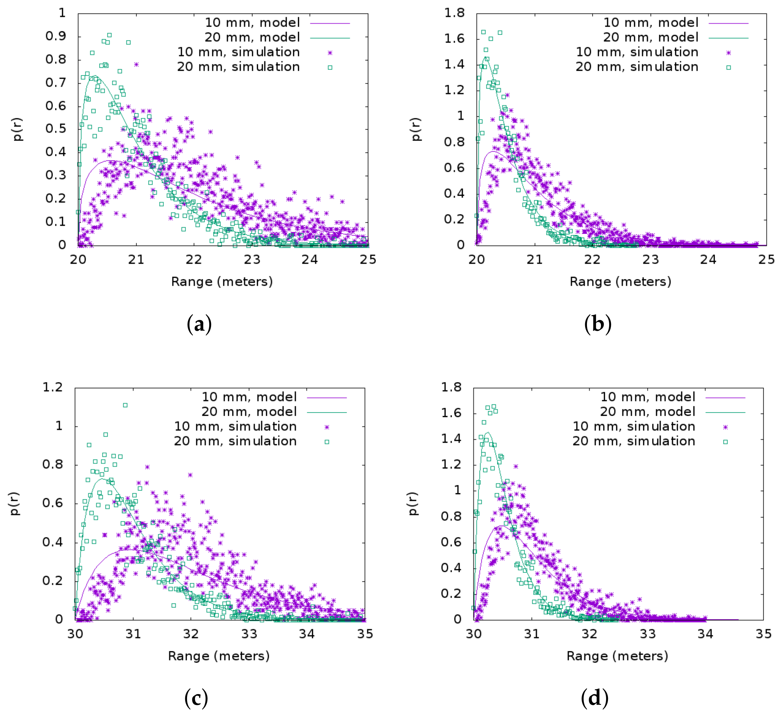
In order to compare the simulation to this model, a single point LIDAR with a divergence of 1 mrad aimed at a stand of randomly placed grass, modeled as uniform vertical cylinders, was simulated. For purposes of comparison, the signal cutoff parameter was set to a value of 100 m, simply because the analytical model does not account for signal cutoff. The grass stand was 10 m wide and 5 m deep. Stem densities of $\lambda =50$ and $\lambda =100$ were simulated, corresponding to 2500 and 5000 stems, respectively, in the 50 m${}^2$ area. The simulation setup is shown in Figure 4.

Simulation results for distances of 20 and 30 m are shown in Figure 5a–d. Several interesting features of the model and simulation are noted. First, increasing the range, D, shifted the entire distribution to the right, as predicted by the model. Second, the most likely value in the simulated distribution matches the model fairly well, although better for the larger grass diameters. Lastly, gamma distribution and the simulation match well qualitatively, indicating that for a diverging beam the gamma distribution is indeed a better predictor of the range statistics than the exponential distribution. The qualitative agreement between the simulation and the analytical model strongly indicates that the simulation is valid for LIDAR-grass interaction for a range of distances and grass properties.

3.4.2. Comparison to Laboratory Experiment

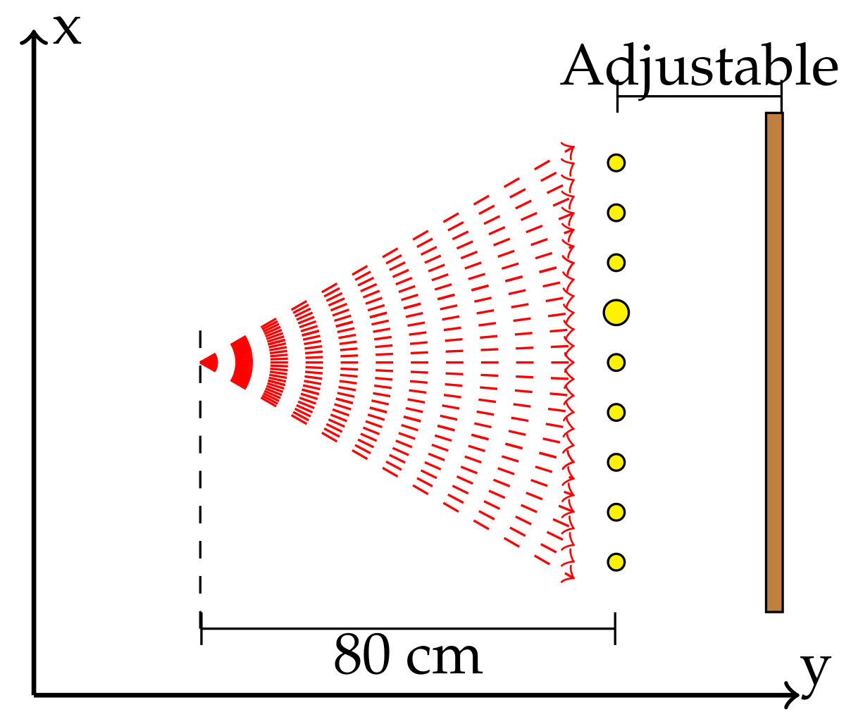
There have been a number of attempts to experimentally quantify the occurrence of mixed pixels in LIDAR measurements. One experiment presented laboratory tests for mixed pixel effects using cylindrical rods arranged in front of a flat background [14]. In the experiment, 8–9 cylindrical rods of various diameters were placed vertically in front of a flat plywood background. While the exact locations and diameters of the rods are not given in the reference, it is possible to infer the approximate arrangement from the figures given in the paper. 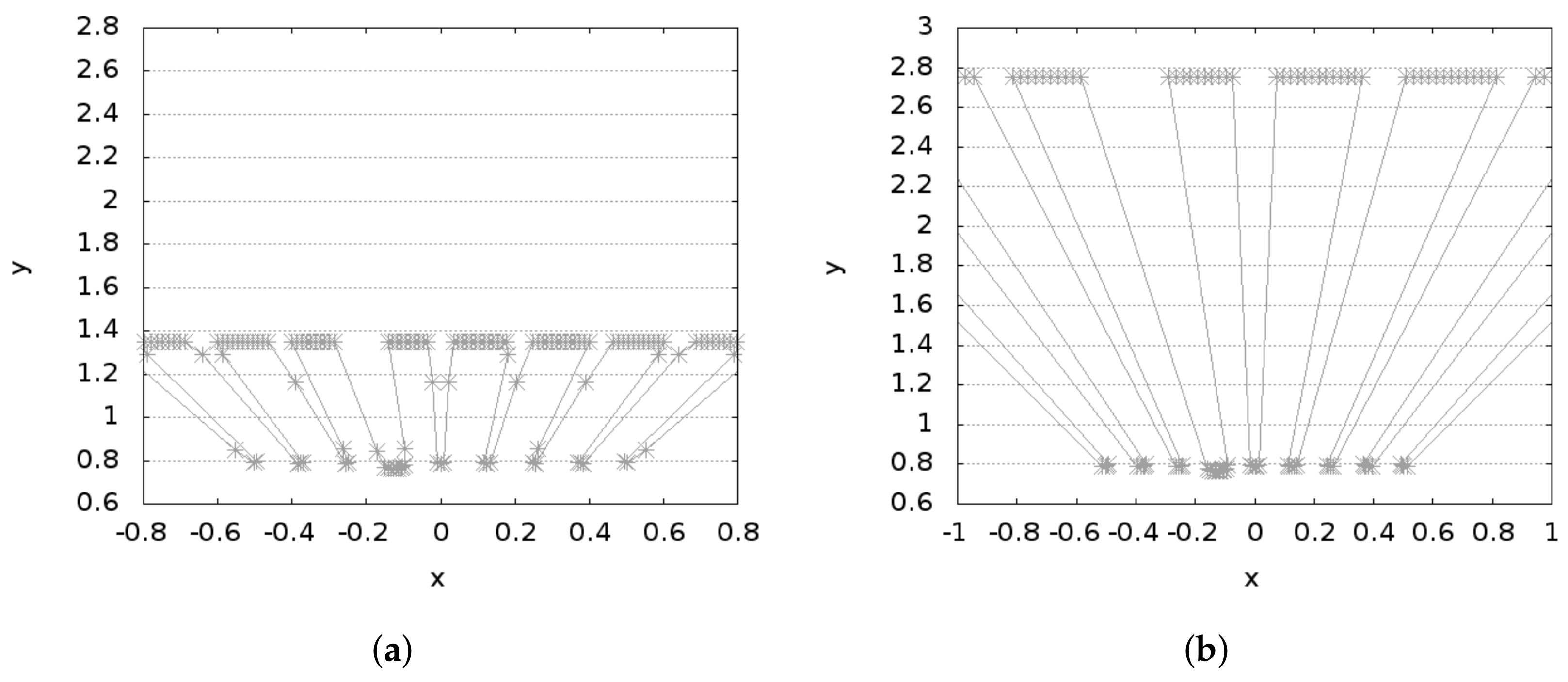Figure 6 shows the arrangement used for the simulations. Nine cylindrical rods were arranged in even 12.7 cm spacings in a row parallel to the background. All rods had diameter of 25 mm, except for one which had a diameter of 75 mm. The sensor was placed 80 cm away from the row of rods, and the background was moved to an offset of either 60 cm or 2 m, to match the results given in Figure 4 of [14].

To compare the results of the laboratory simulations, shown in Figure 7a,b, the LMS-291 with settings listed in

Table 3. LIDAR simulation parameters for the LMS-291.

Parameter	LMS-291S05
Horizontal angles	[−50,50]
Horizontal resolution	0.5, 1.0
Vertical angles	-
Vertical resolution	-
Min range	-
Max range	80
Beam spot shape	circular
Horizontal & vertical divergence	0.0129
Signal cutoff	1.6
Mode	first return

was used. The LMS-291, although originally designed for manufacturing applications, was quite common in field robotics for nearly a decade. However, due to a relatively high divergence (>10 mrad) the sensor is especially prone to mixed pixels. The primary conclusion of the original experiment was that mixed pixels were present when the offset between the background and the cylinders is less than 1.6 m, but at larger offsets the mixed pixels are not present. This is due to the timing resolution and signal processing of the sensor. Figure 7a,b present the results of our simulation, and show clearly that results from the original laboratory experiments are qualitatively reproduced by our simulation. This indicates that our simulated beam divergence and signal processing correctly reproduces the real sensor.

3.4.3. Comparison to Controlled Field Test

Velodyne LIDAR sensors have become ubiquitous in field robotics in the last decade [1]. In particular, the availability of accurate, spatially dense point clouds provided with the introduction of the Velodyne HDL-64E enabled tremendous advances in LIDAR-based autonomous navigation [19,20,21,22]. The Velodyne sensors have a more focused beam than the SICK scanners and are thus less prone to mixed pixels. This lead to a higher degree of “penetration” into extended objects such as vegetation. This feature has been exploited to help distinguish vegetation from solid objects in 3D point clouds generated by the Velodyne sensor [20].

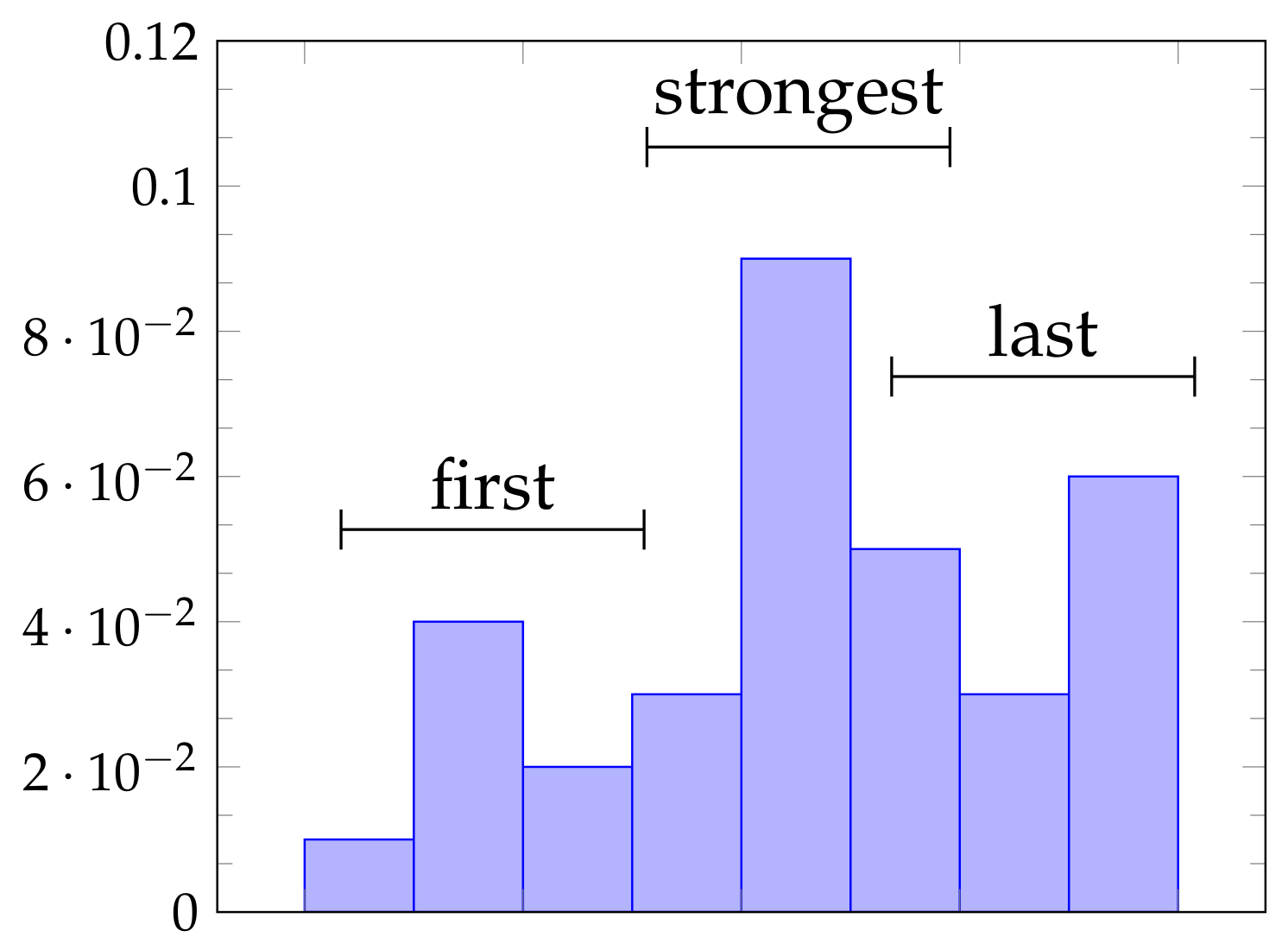
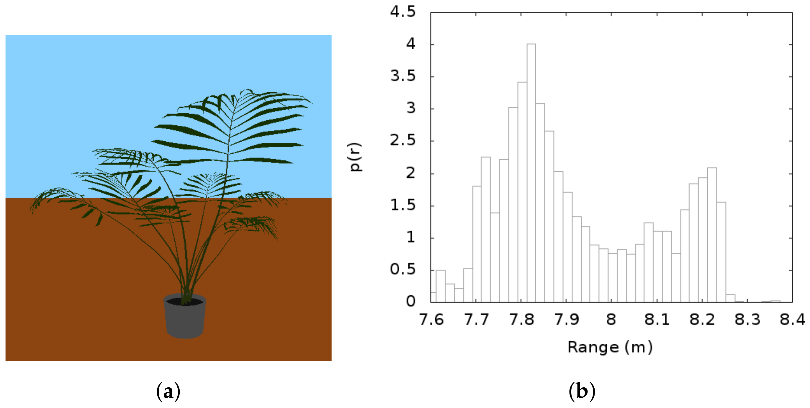
In this section, it is shown that our simulation accurately reproduces sensor-vegetation interaction for the Velodyne HDL-64E. Statistical techniques for quantifying the range penetration properties of LIDAR into vegetation were presented in [23], who showed results for range variability when scanning vegetation with a Velodyne HDL-64E LIDAR. In their experiment, a small potted shrub was placed at a distance of 8 m from the sensor and a histogram of the returned distances from approximately 1500 range measurements was presented. While the experiment cannot be exactly reproduced because the geometric detail about the shrub used in the experiment is not available, the experiment has been reproduced using a shrub model that appears to be a similar size and shape to the one used in [23]. The shrub model used in the experiment is shown in Figure 8a.

In our simulated experiment, the sensor was placed at a distance of 8 m from the shrub shown in Figure 8a and extracted points from one rotation of the sensor on the 5 Hz setting. The sensor was moved along a quarter-circle arc at a distance of 8 m in 1 degree increments, for a total of 91 measurement locations. All distance measurements which returned from the shrub were binned into a histogram, which is shown in Figure 8b. In the original experiments, two main features of the range distribution were observed [23]. First, the broadening of the distribution due to the extended nature of the object, and second the bi-modal nature of the distribution due to some returns from the trunk and others from the foliage. Comparing our Figure 8b to Figure 4 from [23], it is clear that the simulation reproduces both of these features of the distance distribution. This qualitative agreement provides indication that our simulation is valid for Velodyne sensors interacting with vegetation.

3.5. Simulation Demonstration

In this section, the results of an example demonstration in a realistic digital environment are presented. The goal of the demonstration is to show how the simulator could be used to develop and test autonomy algorithms and highlight the LIDAR-vegetation interaction. While the navigation algorithms presented in the demonstration are not novel, the demonstration highlights the efficacy of the sensor simulation for evaluating the navigation algorithm performance and the capability of the simulation to reveal the influence of sensor-environment interaction on autonomous navigation.

3.5.1. Digital Scene

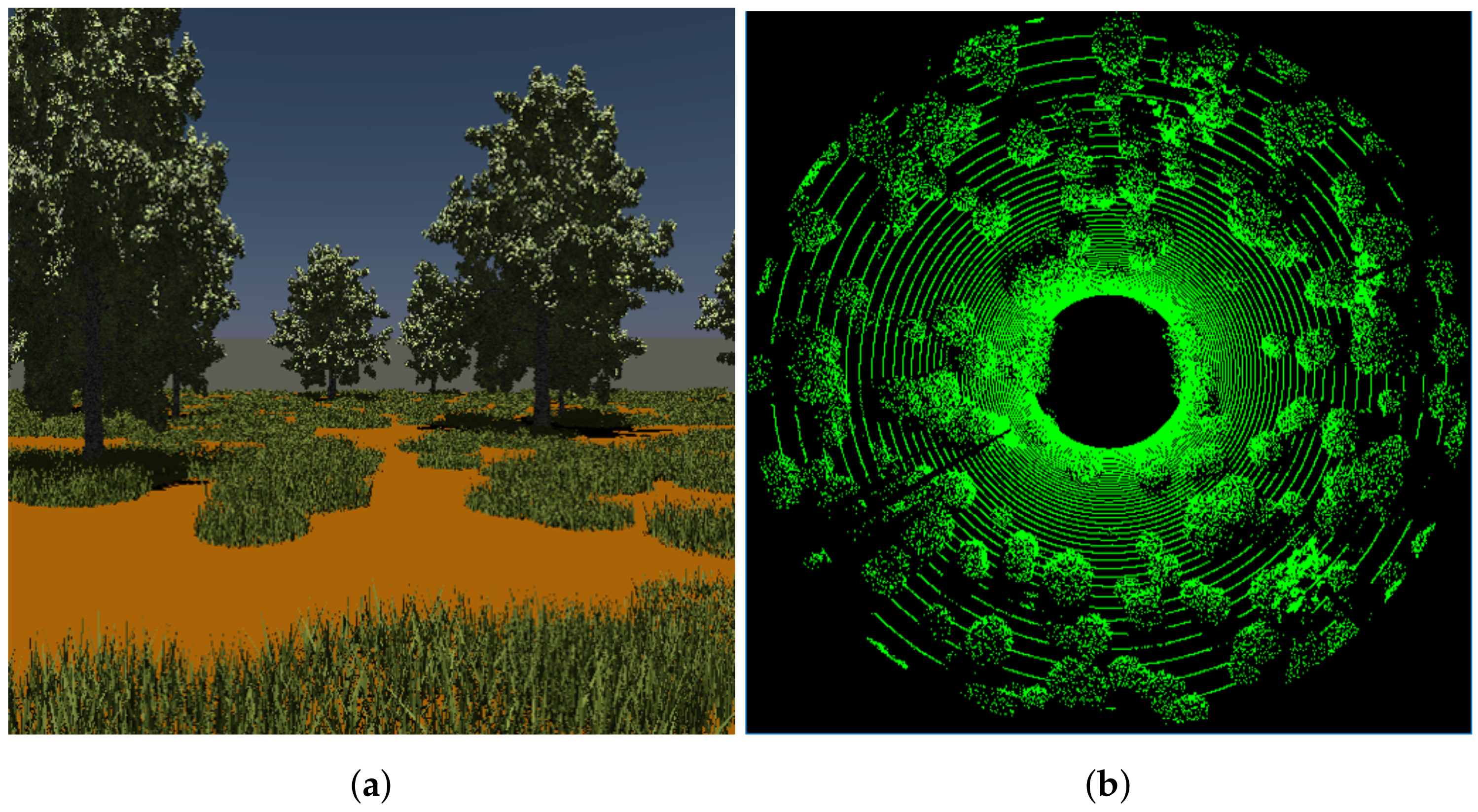
A “courtyard” scene was created by placing vegetation in a 300 × 300 m square, surrounded by a 10 m high wall. One tree model and one grass model were used with random orientations, scales, and locations throughout the courtyard. The resulting scene is shown in Figure 9a. The scene contained nearly 2 million blades of grass, 50 trees, and 191,245,324 triangles. Embree’s instancing feature was used to reduce the memory required to load the scene into the simulation.

3.5.2. Simulating the Velodyne HDL-64E

The Velodyne HDL-64E presents several unique considerations for simulation. First, the sensors consists of two arrays of aligned laser-receiver pairs, with each array having 32 lasers. The lower block of lasers has only one-fourth the horizontal angular resolution of the upper block. The blocks are reported from the sensor in “packets”, and there are three packets from the upper block and then one from the lower block. Finally, because the repetition rate of the laser array is constant, the horizontal resolution of the sensor depends on the rotation rate of the sensor, which can vary from 5–15 Hz.

In order to reproduce these features in the simulation, the upper and lower blocks of the HDL-64E are simulated as two separate LIDAR sensors and combined in the software into a single result. In the simulation, the variable rotation rate, $\omega$, and horizontal resolution (${\delta }^{horizontal}$) are related by the equations

$${\delta }_{lower}^{horizontal}=\frac{360}{\frac{250000}{32\omega }-1}$$

(6)

$${\delta }_{upper}^{horizontal}=\frac{360}{\frac{250000}{8\omega }-1}$$

(7)

In the simulation, the point cloud is assembled from three sets of 32 points from the upper block. The fourth block is discarded from the upper block and replaced by 32 points from the lower block. In this way, the readout and resolution of the real sensor is maintained in the simulation.

Table 4. LIDAR simulation parameters for the Velodyne HDL-64E.

Parameter	Lower Block	Upper Block
Horizontal angles	[−180,180]	[−180, 180]
Horizontal resolution	Equation (6)	Equation (7)
Vertical angles	[−24.8, −11.6127]	[−11.1873, 2.0]
Vertical resolution	0.41875	0.41875
Min range	1	1
Max range	100	100
Beam spot shape	rectangular	rectangular
Horizontal divergence	0.0033	0.0033
Vertical divergence	0.0007	0.0007
Signal cutoff	1.0	1.0
Mode	strongest	strongest

shows how the sensor is parameterized for the simulation. A point cloud from a single simulated scan is shown in Figure 9b.

3.5.3. Simulation Results

In order to demonstrate how the LIDAR simulation could be used to evaluate autonomous performance, an example simulation featuring autonomous navigation with A* [24] is presented. The A* algorithm is a heuristic approach that has been extensively used in autonomous path planning for decades. An implementation based on that by [25] is used in this example. A cost map is created by using scans from the LIDAR sensor. The map had a grid resolution of 0.5 m, and the grid size was 400 × 400. Successive LIDAR scans were registered into world coordinates using a simulated GPS and compass and placed into the grid. Each reflected LIDAR point was assigned a cost, c, based on the point height, h using the formula

$$c=max(100h/h_{max},100)$$

(8)

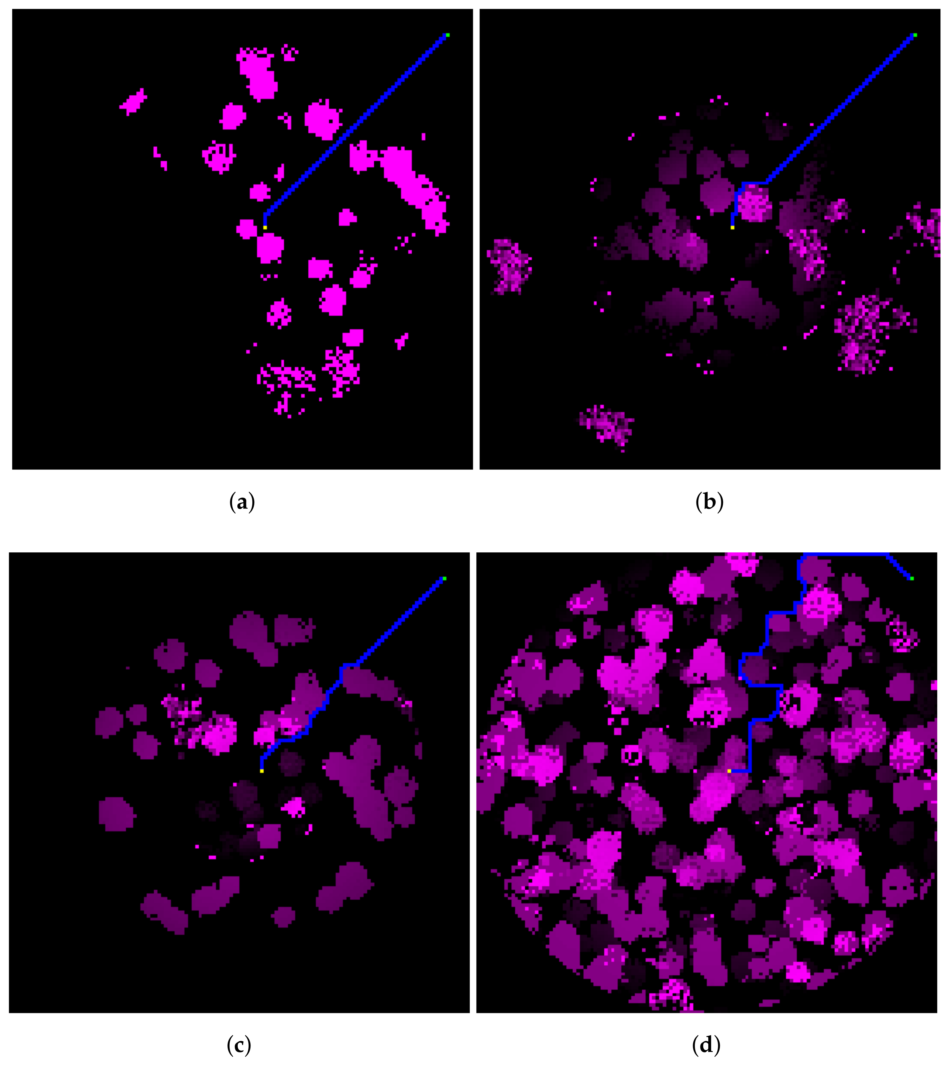
where $h_{max}$ is the maximum negotiable vegetation height of the vehicle. For these simulations, $h_{max}=1.5$. The vehicle was placed in the southwest corner of the scene and given a goal about 130 m northeast of the starting location. The simulated robot was a generic passenger-sized, skid-steered wheeled vehicle with a maximum speed of 2 m/s. The simulation was repeated for four different LIDAR models: the Sick LMS-291 S05, the Velodyne HDL-64E, HDL-32E, and VLP-16. The sensors were mounted on the vehicle at a height of 2 m above the ground. The resulting cost maps after 10 simulated seconds are shown in Figure 10a–d.

Visual comparison of the cost maps and the optimal paths calculated by the A* path planner reveal how the simulator can be used to discover the impact of sensing capability on autonomous performance. The LMS-291, which produces only a horizontal slice of the environment, does not detect most of the grass—it only detects the trees. Additionally, the vegetation that is detected has less range variability within objects—for example compare Figure 10a with Figure 10d. Lack of penetration into vegetation is a well known problem of high-divergence LIDAR like the LMS-291 [3].

There are also clear differences between the cost maps generated by the three Velodyne models. One interesting difference is observed between the VLP-16 and the HDL-64E. While the HDL-64E has a much denser point cloud, the VLP-16 has a much higher maximum opening angle than the HDL-64E (15${}^{\circ }$ above horizontal for the VLP-16 versus 2${}^{\circ }$ above horizontal for the HDL-64E). This results in the VLP-16 detecting tall obstacles at intermediate ranges somewhat better than the HDL-64E. These show up as the ring-like structure in the VLP-16 cost map (Figure 10b). The HDL-64E, however, is better at detecting smaller nearby obstacles. Again, the relative desirability of these features depends on the application, but this demonstration illustrates how the simulation could be used to study autonomous navigation with realistic LIDAR simulations in densely vegetated environments.

3.6. Example of Highly Detailed Digital Environment

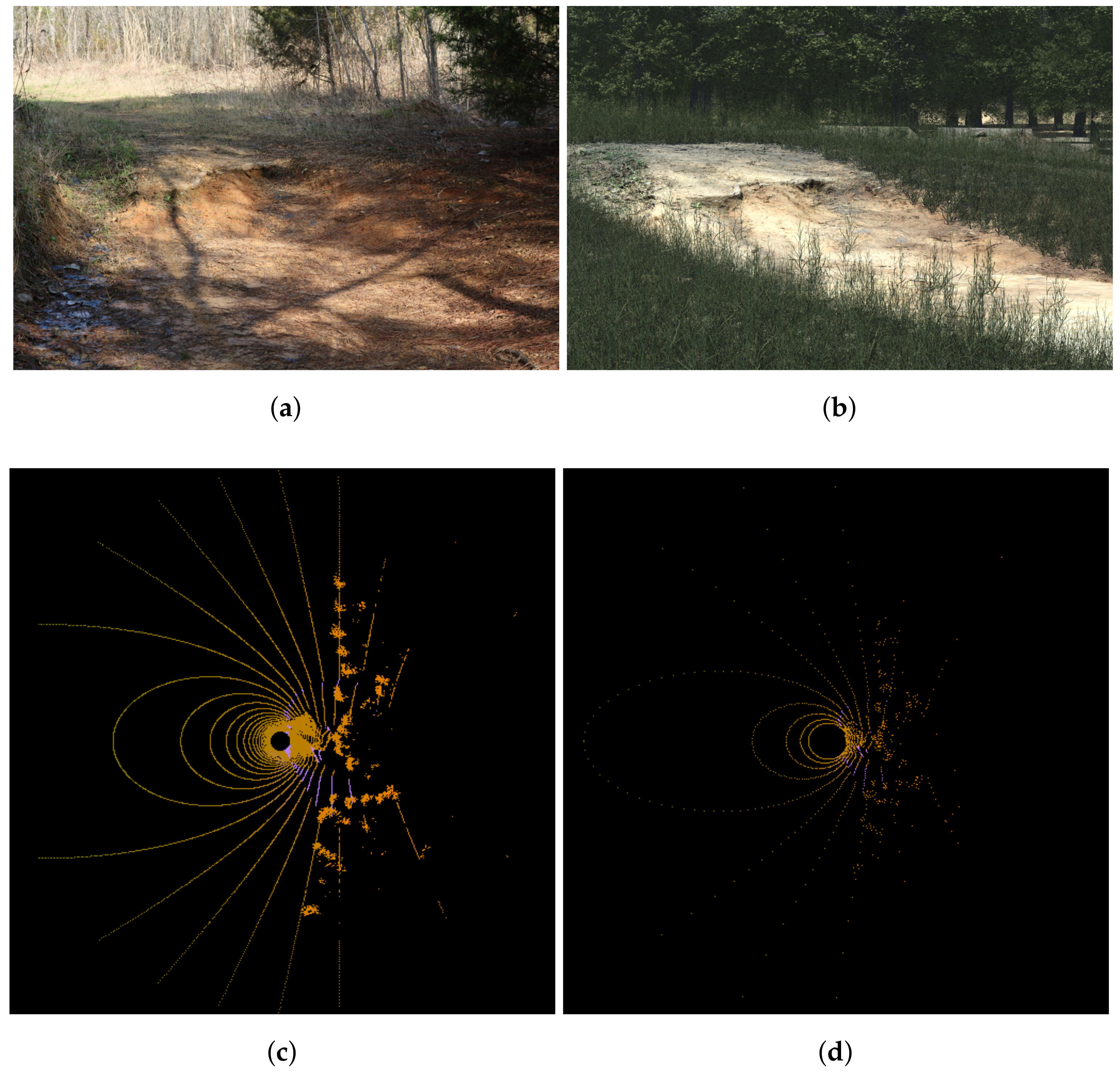
In order to demonstrate how the simulator could be used in real world scenarios, a highly detailed digital scene was developed based on a unique off-road terrain feature. The feature, shown in Figure 11a, is a large vertical step in an off-road trail with a tree root acting as a natural embankment. The geometry of the root feature was measured by developing a structure mesh from a sequence of 268 digital images. The resulting surface mesh contained over 22 million triangular faces and was approximately 2 m by 3 m by 0.4 m in height. The scene was augmented with randomly placed models of grass and trees. The resulting scene contained 24,564 grass and tree meshes for a total of 604,488,350 triangular faces. A digital rendering of the synthetic scene is shown in Figure 11b. Additionally, LIDAR simulations of the scene with two of the sensors discussed in this work are shown in Figure 11c,d as a demonstration of the capability of the LIDAR simulation to scan a complex scene in real-time. The points in Figure 11c,d are color-coded by intensity, and the root feature can be clearly distinguished near the center of each figure.

Although this level of geometrical detail is probably unnecessary for LIDAR simulations, this exercise demonstrates the capability that the simulator has for highly detailed digital terrains for sensor simulations.

4. Discussion

While the design, development, and testing of autonomous ground vehicles is primarily done through physical experimentation, there are obvious benefits to using simulation. A recent paper on simulation of autonomous urban driving systems stated several disadvantages of physical testing [26], including infrastructure cost, logistical difficulties, and inability to perform a statistically significant number of experiment for training and validation of autonomous algorithms.

Additionally, many important safety scenarios, such as pedestrian detection and avoidance, are dangerous or impractical to study in physical experiments. There is therefore a growing body of research on the use of simulation for the development, training, and testing of autonomous navigation algorithms for passenger-sized vehicles [5,6,7,26,27]. The simulator presented in this work adds to this growing field in the area of off-road autonomous navigation by providing a methodology for realistic, real-time simulation of LIDAR-vegetation interaction. This new capability can improve both the development and testing of off-road autonomous systems.

While simulation can never fully replace field testing, simulation offers several advantages over field testing. First, the simulation environment is known and controlled, meaning environmental factors can be controlled and eliminated as a source of variability in testing if desired. Second, simulation offers the ability to have perfect knowledge of “ground truth”, which can make training and testing detection and classification algorithms much simpler and faster.

Simulation tools for autonomous ground robotics can be typically divided into three broad categories, based on the physical-realism, environmental fidelity, and the purpose of the simulator. The first category of simulations are what one 2011 review called “Robotic Development Environments” (RDE) [28]. These include Gazebo [29], USARSIM [30], Microsoft Robotics Developer Studio [31], and other simulators used to interactively design and debug autonomous systems in the early stage of development. Other more recent examples include customized simulations with simplified physics for closed-loop autonomy simulations in MATLAB [32,33].

While many of these tools are now defunct or unsupported due to the popularity of Gazebo, they share several traits in accordance with their intended use. First, RDE focus on ease of use and integration into the robotic development process—undoubtedly a reason behind Gazebo’s overwhelming popularity. Second, these simulators tend to avoid detailed simulation of the environment and the robot-environment interaction because this is outside the scope of their intended use. Last, RDE typically simulate in real-time or faster, allowing robotic developers to quickly design, develop, and debug autonomous systems.

The second category of robotic simulator could be called “Robotic Test Environments” (RTE), in keeping with the above nomenclature. Simulators such as the Virtual Autonomous Navigation Environment (VANE) [34], MODSIM [35], Robotic Interactive Visualization Experimentation Technology (RIVET) [36], the Autonomous Navigation Virtual Environment Laboratory (ANVEL) [37], and the CARLA [26] fall into this category. RTE are typically used to evaluate the performance of a robotic system in a realistic operational setting—necessitating a higher degree of realism in the robot-environment interaction physics. Even among RTE there is a wide range of realism in the sensor-environment interaction physics, depending on the application. For example, the RIVET, which is primarily used to study human-robot interaction, has lower-fidelity sensor simulations than then ANVEL, which has been used to evaluate mission effectiveness. The VANE has the most realistic LIDAR-environment interaction physics [38,39], but runs much slower than real-time.

The third class of simulators are empirical or semi-empirical simulators. These range from software that simply replays modified data collected in previous experiments to complex models developed from field data. For example, a realistic simulation of a Velodyne HDL-64E interacting with vegetation was developed by quantifying the statistics of LIDAR-vegetation interaction for a sensor in a particular environment and then digitizing the environment based on those statistics [23,40]. More recently, much attention has been given to Waymo’s Carcraft simulator, which uses a mixture of real and simulated data to virtualize previously measured events [27]. These empirical simulators can be quite realistic when predicting the performance of a specific autonomous system in a particular environment and are therefore useful in robotic development projects which already feature extensive field testing. However, these empirical simulators cannot fill the need for predictive, physics-based modeling [41].

In this context, the LIDAR simulation presented in this paper is unique because it provides a more realistic model of the LIDAR-vegetation interaction than any of the other real-time simulators, but still maintains real-time or faster-than real-time computational performance. This work enables predictive, interactive simulations of robotic performance in realistic outdoor environments to be integrated into human-in-the-loop or hardware-in-the-loop testing of autonomous systems in complex outdoor environments.

5. Conclusions

In conclusion, this work has documented the development and validation of a high-fidelity, physics-based LIDAR simulator for autonomous ground vehicles that can be used to simulate LIDAR sensors interacting with complex outdoor environments in real-time.

The value of this capability in the development and testing of autonomous systems, as well as the improvements over past simulators, was presented in Section 4.

Future work will enhance the simulator in several ways. First, the interaction of the LIDAR with dust, snow, rain, and fog—all of which can adversely affect LIDAR performance—will be incorporated. Additionally, the environment representation will be enhanced to include retro-reflective surfaces like road signs.