Abstract
Simultaneous polarimetric radar transmits a pair of orthogonal waveforms both of which must have good auto- and cross-correlation properties. Besides, high Doppler tolerance is also required in measuring the highly maneuvering targets. A new method for the design of sequences with good correlation and Doppler properties is proposed. We formulate a fourth-order polynomial, but unconstrained, minimization problem. An iterative algorithm based on the gradient method on the phases is applied to solve it. Numerical results demonstrate the superiority of the proposed algorithm compared to the previous state-of-the-art method.
1. Introduction
In recent years, the simultaneous polarimetric scheme has been widely used to obtain accurate polarization features, which can be described by a second-order polarization scattering matrix (PSM), of targets [1,2,3,4]. A pair of waveforms transmitted in this mode is required to be stringently orthogonal, which is usually evaluated by the Isolation of the waveforms, to reduce the interference caused by simultaneous transmission and reception [4]. Meanwhile, the autocorrelation properties of the sequences, which usually represent the peak side-lobe level (PSL) and the integrated side-lobe level (ISL), are also of great importance [5]. Generally, the peak of the sidelobes corresponds to falsely detected objects, while high PSL result in masking of the weak targets with small radar cross-section (RCS) next to high signature targets in nearby range cells. Besides, for typical use of the polarimetric radar in meteorology, the ISL is an important metric. In [6,7,8], it has been pointed out that the targets for weather radar are extended volume scatterers and range sidelobes are a major source of error for quantitative applications. Therefore, designing waveforms with good correlation (in the rest of the article, correlation is used to denote both auto- and cross-correlation) properties is of great significance for simultaneous polarimetric radar.
Sequences design with good correlation properties is a traditional problem in radar and communication systems [9,10,11,12]. Focusing on the designing problem, numerous algorithms have been proposed to design the sequences. Among these techniques, a class of typical methods to design the sequences is to use the intelligent algorithms directly. Deng et al. designed unimodular sequences by using Simulated Annealing algorithm and analysed the performance of the sequences in applications of orthogonal netted radar [13]. In addition, Liu et al. used genetic algorithm to obtain sequences with good correlation properties [14]. However, the correlation properties, including PSL and Isolation of the results designed by the above-mentioned algorithms will become worse than the theoretical limiting performance with the sequences length increasing [15,16]. Besides, many researchers have also proposed computationally efficient cyclic optimization algorithms for the design of unimodular sequences. Following a similar line of derivation, Stoica et al. proposed a series of four algorithms containing CAP, CAN, WeCAN and CAD [17], which are based on the minimization of ISL with high computational efficiency. Meanwhile, these procedures can optimize the specified part of the correlation function. It should be pointed out that in some cases, the interest lies in making partial sidelobes small rather than making all sidelobes small [5,15]. However, the practical convergence rate of these four algorithms becomes slow with the sequences length increasing. Based on a customized Limited-Memory Broyden Fletcher Goldfarb and Shanno (LBFGS) algorithm, the problem of minimizing the concerned sidelobes of the correlation function is addressed by Wang et al. in [18]. By defining a new correlation matrix and using the Fast Fourier Transforms (FFT) algorithm, they moderated the computational complexity and improved the convergence rate of the method compared to the WeCAN algorithm. In a recent work [5], Palomar et al. developed the general majorization-minimization (MM) method to tackle the optimization problem arising from the sequences design. By means of the FFT algorithm, they solve the problem of designing sets of very long sequences. However, like LBFGS and MM methods, the Doppler tolerance of the sequences is not considered. In other words, they lack the ability to optimize the Doppler tolerance of the sequence sets.
In [19], Kretschmer et al. have proved that the correlation performance of the phase-coded sequences is sensitive to the target velocity. Even if the target velocity is low, the PSL and Isolation of the waveforms will seriously deteriorate compared with the same metrics of the static target’s echoes. Focusing on this problem, Pezeshki et al. investigated the Doppler tolerant waveforms designing problem for the polarimetric radar [20,21,22]. The constituent waveforms are Golay complementary codes, which have been used in many active sensing and communication systems, for instance, radar pulse compression [23], orthogonal frequency-division multiplexing (OFDM) [24] and channel estimation [25], because of the perfect autocorrelation properties along the zero Doppler shift. Based on the Prouhet-Thue-Morse sequence, they constructed Doppler resilient sequences and the range sidelobes almost vanished at modest Doppler shifts. However, the cross-correlation properties of the sequences cannot be optimized by their methods. Meanwhile, the correlation properties of the sequences keep good only in a small Doppler shifts interval around the zero Doppler shift. Their method lacks the ability to design sequences with good correlation properties in specific range and Doppler bins of the ambiguity function. In [26], Cui et al. considered the local ambiguity function shaping and proposed an accelerate iterative sequential optimization (AISO) algorithm to minimized the average value of the weighted integrated sidelobe level (WISL) over specific Doppler bins and range bins of interest. However, the orthogonality of the sequences that is of great importance for simultaneous polarimetric radar is not considered in AISO algorithm.
In this article, based on the gradient method shown in [18,27], we propose a new cyclic algorithm that can design sequences not only with good correlation properties but also with high Doppler tolerance. The obtained sequences can be used for the space surveillance radar to improve the measurement accuracy of the PSM of the highly maneuvering targets, including satellites, spacecraft, etc. The proposed method can be summarized as follows:
- Suppressing a specific part of the correlation function
- Good correlation properties under motion states of interest
- Better sidelobes both in terms of PSL and ISL
The remainder of this paper is organized as follows: the problem for designing sequences with good correlation and Doppler properties is formulated in Section 2; in Section 3, the Iterative Algorithm–Gradient (IAG) algorithm is proposed to solve the design problem; simulations are presented to validate the method in Section 4; and Section 5 concludes the paper.
: In this paper, it is assumed that a lower-case letter (e.g., a) denotes a scalar; a boldface lower-case letter (e.g., ) denotes a vector; and a boldface upper-case letter (e.g., ) indicates a matrix. Additionally, the symbols and represent transpose and conjugate transpose of the matrix , respectively. and indicate the absolute value and the conjugate of the scalar a. Besides, denotes the Frobuinous norm of a matrix and ⊙ represents the Hadamard product of two matrices with the same dimension. represents the real part of the scalar a and denotes the trace of the matrix .
2. Problem Formulation
A pair of constant modulus sequences used for simultaneous polarimetric radar can be written as
where
are the sequences to be designed (it is assumed that the phases can be arbitrary values from ), H and V represent the horizontal and vertical polarized channels, is the time duration of one subpulse and is the shaping function, e.g., a rectangular pulse with amplitude 1. When the target moves, the Doppler shift of the received signals in different times is
where is the carrier wavelength, and are the radial velocity and acceleration, respectively, the subscript l represents the motion state of interest, and L is the amount of the concerning motion states. The (aperiodic) correlation of and (in the rest of the paper, are both used to denote H and V) is defined as
When , (4) becomes the autocorrelation of . Denote the transmitted sequences by an N-by-2 matrix
and the Doppler echoes sequences by an N-by- matrix
where
and
Then, the correlation entries for the kth lag in (4) are given by the elements of the following correlation matrix [18]
where
and is the identity matrix. It should be noted that the elements of are made up of the autocorrelations and cross-correlations of the sequences. A compact optimization model for deigning constant modulus sequences with low correlation sidelobes levels can be formulated as
where
and is the impulse function, i.e., for and otherwise . In (11), are positive real weights chosen by the user, and is also a preset positive integer, which represents the lag interval of interest. The model (11) involves minimizing a fourth-order polynomial with nonlinear equality constraints, which is numerically difficult to handle. However, using the phases as new variables, the constant modulus constraints can be dropped and (11) can be formulated as an unconstrained fourth-order polynomial minimization problem
where
Compared with (11), obtaining the global optimal solution of (13) is still a NP-hard problem. However, considering the local optimal solutions, it is easier to handle the optimization problem. In this paper, an iterative algorithm based on the gradient method, which can be applied directly, is proposed to solve the problem of (13). In the gradient method, the consuming time of each iteration is determined by the calculation of and . The computational costs of calculating and directly are and , respectively, according to (13) [18]. In the following, an efficient method is proposed to compute them.
3. Solving the Model by IAG Algorithm
Introducing the notation, the matrix is defined as
where , and vectorizes a matrix by stacking its columns on top of one another. Then the function can be rewritten as
where and denotes the 2-norm of a vector. According to (16), the gradient can be computed as follows:
Furthermore, it should be noted that each row vector of can be computed by the convolution product, , where the sequence can be obtained by reversing the order of the entries of . In other words, the entries in , and can be computed by truncating from the indices to G. Besides, the convolution operation in the time domain corresponds to the product operation in the frequency domain. Thus, the FFT algorithm can be applied to obtain , and by complex multiplication operations at most. Computing takes complex multiplication operations. So the computation cost of obtaining is . As for , there are entries. According to (4), for (the same as ), it should be noticed that
and
The entries in , and can be obtained according to (19) and (21), and correspondingly, it takes complex multiplication operations. Thus, the computational cost of is . The computational complexities to compute and using the original expression (13) and new expression (16) are shown in Table 1. Furthermore, using the gradient , the following IAG algorithm shown in Table 2 can be performed to obtain the sequences with good correlation properties and high Doppler tolerance. One thing should be pointed out is that for the classical gradient method, the line search rule is based on the Wolfe conditions which can ensure the stability of the iterations. In this paper, to improve the efficiency of the algorithm, a low computation complexity line search rule, named Armijo-rule, is used [28].

Table 2.
Steps for the IAG algorithm.
4. Numerical Results
Here, we provide numerical examples to illustrate the performance of the proposed IAG algorithm. The state-of-the-art WeCAN algorithm proposed in [17] is considered for comparison. The metrics Peak Side-lobe Level (), Integrated Side-lobe Level () and the Isolation (I) are used to evaluate the performance of the sequences which are defined as follows [4]
The running time is obtained using the Matlab 2016b version, running on a standard PC (with a 2.6 GHz Core i7 CPU and 4-GB RAM).
In the first numerical example, we consider the measurement of the stationary target, meaning the Doppler shift in (3) is zero. Simulation parameters are shown in Table 3. Assume the sequence length is and the lag interval of interest is . The weight coefficients are for the IAG method. For the WeCAN algorithm, the parameter should be large enough to guarantee the stability of the algorithm. Thus, the weights are set as 30 while and 1 while for the WeCAN method. The predefined threshold of the predefined threshold is for the two methods. To avoid unreasonable solution, the minimum iteration number is set to 1000 in the simulations.
Table 3.
Simulation parameters for the first example.
Figure 1a,b show the convergence curves of the two algorithms. The convergence rate of the and I of the IAG method is much faster than that of the WeCAN method. The and I of the sequences designed by the IAG method achieve about after 700 iterations, however, the corresponding number of iterations is over for the WeCAN method. Further, Figure 2a,b illustrate the correlation level of the sequences designed by the two methods. The and I of the IAG sequences are about better than that of the WeCAN sequences with under this situation. Meanwhile, the is for IAG and for WeCAN, which indicates the energy of the sidelobes is lower for IAG sequences. In other words, the IAG sequences are suitable for observing the volume targets that extend over range areas. The consuming time and iteration number are shown in the Table 4. It can be observed that the average execution time of per iteration of the IAG method is shorter than that of the WeCAN method. As mentioned before, by the new expression (16) and the using of FFT, the consuming time for computing the objective function and the corresponding gradient becomes less, leading the average execution time of the IAG method shorter. Meanwhile, the IAG method takes much less iterations than the WeCAN method. Thus, the total execution time is less than one in a hundred in comparison with that of the WeCAN method.
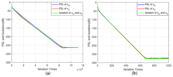
Figure 1.
The convergence curves of the WeCAN approach and the IAG approach. (a) WeCAN; (b) IAG.
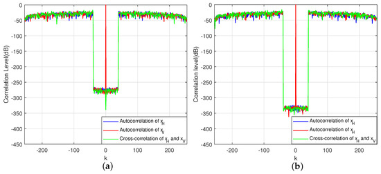
Figure 2.
The correlation levels of the WeCAN approach and the IAG approach. (a) WeCAN; (b) IAG.
Table 4.
Comparison between IAG and WeCAN.
In the second numerical example, designing sequences for measuring the polarization features of the highly maneuvering target is simulated. In [29], Li has pointed out that typical highly maneuvering targets contain satellites, spacecrafts, etc. The velocity of these targets is usually about Mach 10 or even higher. Meanwhile, the acceleration is about (g is the acceleration of gravity). Thus, in the simulations, the velocity and the acceleration of the target are assumed to be within and , respectively. We uniformly discretize the velocity and acceleration intervals into L bins with the grid size and . Then the motion states of interest in (3) can be expressed as the column of the following matrix .
where the amount of concerning motion states L can be computed as
Other simulation parameters are shown in Table 5. The first four parameters are same as those in Table 3. Besides, taking typical simultaneous polarimetric radars, including the MERIC radar [30] and the CSU-CHILL radar [31], as references, the carrier frequency is set to . The carrier wavelength in (3) can be computed by , where c is the speed of light. The time duration of the subpulse is . Then the IAG algorithm shown in Table 2 can be performed to obtain the sequences with good correlation properties under the motion states of interest. Figure 3 and Figure 4 show the correlation properties of the designed sequences designed by the IAG and WeCAN algorithms through the metrics and I, respectively. It clearly demonstrates that the correlation properties of the sequences designed by the IAG method are better than that of the sequences designed by the WeCAN method under the given motion states. Correspondingly, the and I of the IAG sequences are under , however, the same metrics of the WeCAN sequences are about in this situation. The as a function of velocity and acceleration is shown in Figure 5. It can be observed that under the same conditions, the of the IAG sequences is about one in a thousand in comparison with that of the WeCAN sequences. The reason is that the influence of the velocity and the acceleration of the target on the correlation properties of the sequences, which is not considered in the WeCAN method, is taken into account in the objective function (11) of the IAG method. Besides, it can be observed that the metrics, including , and I, change slightly with the acceleration increasing. Since the time duration of the subpulse is set to in the simulation, the time length of the sequence is equal to , which is quite small in this situation, leading the slight change of the velocity. Thus, the properties of the sequences change slightly with the increasing of the acceleration.
Table 5.
Simulation parameters for the second example.
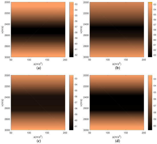
Figure 3.
The and I of the sequences designed by the IAG algorithm (dB). (a) The of under different motion states; (b) The of under different motion states; (c) The I of under different motion states; (d) The I of under different motion states.
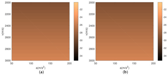
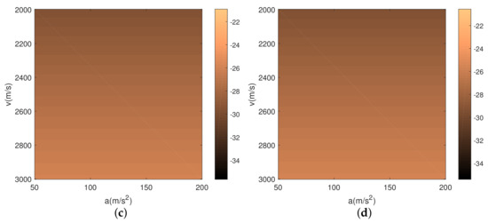
Figure 4.
The and I of the sequences designed by the WeCAN algorithm (dB). (a) The of under different motion states; (b) The of under different motion states; (c) The I of under different motion states; (d) The I of under different motion states.
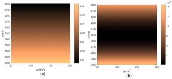
Figure 5.
The of the sequences designed by the WeCAN algorithm and the IAG algorithm under different motion states. (a) WeCAN; (b) IAG.
5. Conclusions
In this paper, we propose an iterative algorithm based on the gradient method to design the constant modulus sequences with good correlation and Doppler properties for simultaneous polarimetric radar. By transforming the objective function to a new expression, the computation complexities of the gradient and the objective function are reduced by using the FFT algorithm. Compared with the state-of-the-art WeCAN approach, the proposed IAG method has a better performance in terms of correlation sidelobes levels, Doppler tolerance and execution time.
Author Contributions
F.W. proposed the original idea of this paper; X.W. and C.P. conceived and designed the experiments; F.W. performed the experiments; F.W. and Y.L. analyzed the data; F.W. wrote the paper.
Funding
This research was funded by the National Natural Science Foundation of China, grant numbers 61490690, 61490694 and 61701512.
Conflicts of Interest
The authors declare no conflict of interest.
References
- Wang, F.; Li, C.; Pang, C.; Li, Y.Z.; Wang, X.S. A Method for Estimating the Polarimetric Scattering Matrix of Moving Target for Simultaneous Fully Polarimetric Radar. Sensors 2018, 18, 1418. [Google Scholar] [CrossRef] [PubMed]
- Yanovsky, F.J.; Russchenberg, H.W.J.; Unal, C.M.H. Retrieval of information about turbulence in rain by using Doppler-polarimetric radar. IEEE Trans. Microw. Theory Tech. 2005, 53, 444–450. [Google Scholar] [CrossRef]
- Wang, F.; Pang, C.; Li, Y.Z.; Wang, X.S. Algorithms for Designing Unimodular Sequences with High Doppler Tolerance for Simultaneous Fully Polarimetric Radar. Sensors 2018, 18, 905. [Google Scholar] [CrossRef] [PubMed]
- Giuli, D.; Fossi, M.; Facheris, L. Radar target scattering matrix measurement through orthogonal signals. IEE Proc. F Radar Signal Process. 1993, 140, 233–242. [Google Scholar] [CrossRef]
- Song, J.; Babu, P.; Palomar, D.P. Sequence set design with good correlation properties via majorization-minimization. IEEE Trans. Signal Process. 2016, 64, 2866–2879. [Google Scholar] [CrossRef]
- Cilliers, J.E.; Smit, J.C. Pulse Compression Sidelobe Reduction by Minimization of Lp-Norms. IEEE Trans. Aerosp. Electron. Syst. 2007, 43, 1238–1247. [Google Scholar] [CrossRef]
- Mishra, K.V. Frequency Diversity Wideband Digital Receiver and Signal Processor for Solid-State Dual-Polarimetric Weather Radars. Ph.D. Thesis, Colorado State University, Fort Collins, CO, USA, 2012. [Google Scholar]
- Bharadwaj, N.; Mishra, K.V.; Chandrasekar, V. Waveform considerations for dual-polarization Doppler weather radar with solid-state transmitters. In Proceedings of the IEEE International Geoscience and Remote Sensing Symposium, Cape Town, South Africa, 12–17 July 2009; pp. 267–270. [Google Scholar]
- Boehmer, A.M. Binary pulse compression codes. IEEE Trans. Inf. Theory 1967, 13, 156–167. [Google Scholar] [CrossRef]
- Baden, J.M. Efficient optimization of the merit factor of long binary sequences. IEEE Trans. Inf. Theory 2011, 57, 8084–8094. [Google Scholar] [CrossRef]
- Xiong, T.; Hall, J. Construction of even length binary sequences with asymptotic merit factor 6. IEEE Trans. Inf. Theory 2008, 54, 931–935. [Google Scholar] [CrossRef]
- Chu, D. Polyphase codes with good periodic correlation properties (corresp.). IEEE Trans. Inf. Theory 1972, 18, 531–532. [Google Scholar] [CrossRef]
- Deng, H. Polyphase code design for orthogonal netted radar systems. IEEE Trans. Signal Process. 2004, 52, 3126–3135. [Google Scholar] [CrossRef]
- Liu, B.; He, Z.S. Orthogonal Discrete Frequency-Coding Waveform Set Design with Minimized Autocorrelation Sidelobes. IEEE Trans. Aerosp. Electron. Syst. 2009, 45, 1650–1657. [Google Scholar] [CrossRef]
- Mohammad, A.K.; Augusto, A.; Antonio, D.; Mohammad, M.N.; Mahmoud, M.H. A Coordinate-Descent Framework to Design Low PSL/ISL Sequences. IEEE Trans. Signal Process. 2017, 65, 5942–5956. [Google Scholar]
- Nasrabadi, M.; Bastani, M. A Survey on the Design of Binary Pulse Compression Codes with Low Autocorrelation; INTECH: Rijeka, UK, 2010. [Google Scholar]
- He, H.; Stoica, P.; Li, J. Designing unimodular sequences sets with good correlations-Including an application to MIMO radar. IEEE Trans. Signal Process. 2009, 57, 4391–4405. [Google Scholar] [CrossRef]
- Wang, Y.C.; Dong, L.; Xue, X.; Yi, K.C. On the Design of Constant Modulus Sequences with Low Correlation Sidelobes Levels. IEEE Signal Process. Lett. 2012, 16, 462–465. [Google Scholar] [CrossRef]
- Kretschmer, F.F.; Lewis, B.L. Doppler properties of poly-phase coded pulse compression waveforms. IEEE Trans. Aerosp. Electron. Syst. 1983, 19, 521–531. [Google Scholar] [CrossRef]
- Pezeshki, A.; Calderbank, A.R.; Moran, W.; Howard, S.D. Doppler Resilient Golay Complementary Waveforms. IEEE Trans. Inf. Theory 2008, 54, 4254–4266. [Google Scholar] [CrossRef]
- Pezeshki, A.; Calderbank, A.R.; Howard, S.D.; Moran, W. Doppler Resilient Golay Complementary Pairs for Radar. In Proceedings of the IEEE/SP, Workshop on Statistical Signal Processing, Madison, WI, USA, 26–29 August 2007; pp. 483–487. [Google Scholar]
- Pezeshki, A.; Calderbank, A.R.; Moran, W.; Howard, S.D. Doppler Resilient Waveforms with Perfect Autocorrelation. arXiv. 2007. Available online: https://arxiv.org/abs/cs/0703057 (accessed on 12 July 2018).
- Levanon, N. Noncoherent radar pulse compression based on complementary sequences. IEEE Trans. Aerosp. Electron. Syst. 2009, 45, 742–747. [Google Scholar] [CrossRef]
- Schmidt, K. Complementary sets, generalized Reed-Muller codes, and power control for OFDM. IEEE Trans. Inf. Theory 2007, 53, 808–814. [Google Scholar] [CrossRef]
- Mishra, K.V.; Eldar, Y.C. Sub-Nyquist channel estimation over IEEE 802.11ad link. In Proceedings of the International Conference on Sampling Theory and Applications, Tallinn, Estonia, 3–7 July 2017; pp. 355–359. [Google Scholar]
- Cui, G.; Fu, Y.; Yu, X.; Li, J. Local Ambiguity Function Shaping via Unimodular Sequence Design. IEEE Signal Process. Lett. 2017, 24, 977–981. [Google Scholar] [CrossRef]
- Arriaga, I.A.; Orozco, A.; Flores, J. Design of Unimodular Sequences with Good Autocorrelation and Good Complementary Autocorrelation Properties. IEEE Signal Process. Lett. 2017, 24, 1153–1157. [Google Scholar] [CrossRef]
- Yuan, Y.X.; Sun, W.Y. Optimization Theory and Method; Science Press: Beiing, China, 2006; pp. 94–100. [Google Scholar]
- Li, W.C. Radar Signal Parameter Estimation and Image Processing of High-speed Maneuvering Target. Ph.D. Thesis, National University of Defense Technology, Hunan, China, 2009. [Google Scholar]
- Titinschnaider, C.; Attia, S. Calibration of the MERIC full-polarimetric radar: theory and implementation. Aerosp. Sci. Technol. 2003, 7, 633–640. [Google Scholar] [CrossRef]
- Hubbert, J.; Bringi, V.N.; Carey, L.D.; Bolen, S. CSU-CHILL Polarimetric Radar Measurements from a Severe Hail Storm in Easter. J. Appl. Meteorol. 1996, 37, 749–775. [Google Scholar] [CrossRef]
© 2018 by the authors. Licensee MDPI, Basel, Switzerland. This article is an open access article distributed under the terms and conditions of the Creative Commons Attribution (CC BY) license (http://creativecommons.org/licenses/by/4.0/).