Supercapacitor Electro-Mathematical and Machine Learning Modelling for Low Power Applications

 ,
,
Abstract
1. Introduction
2. Related Work at Different Techniques
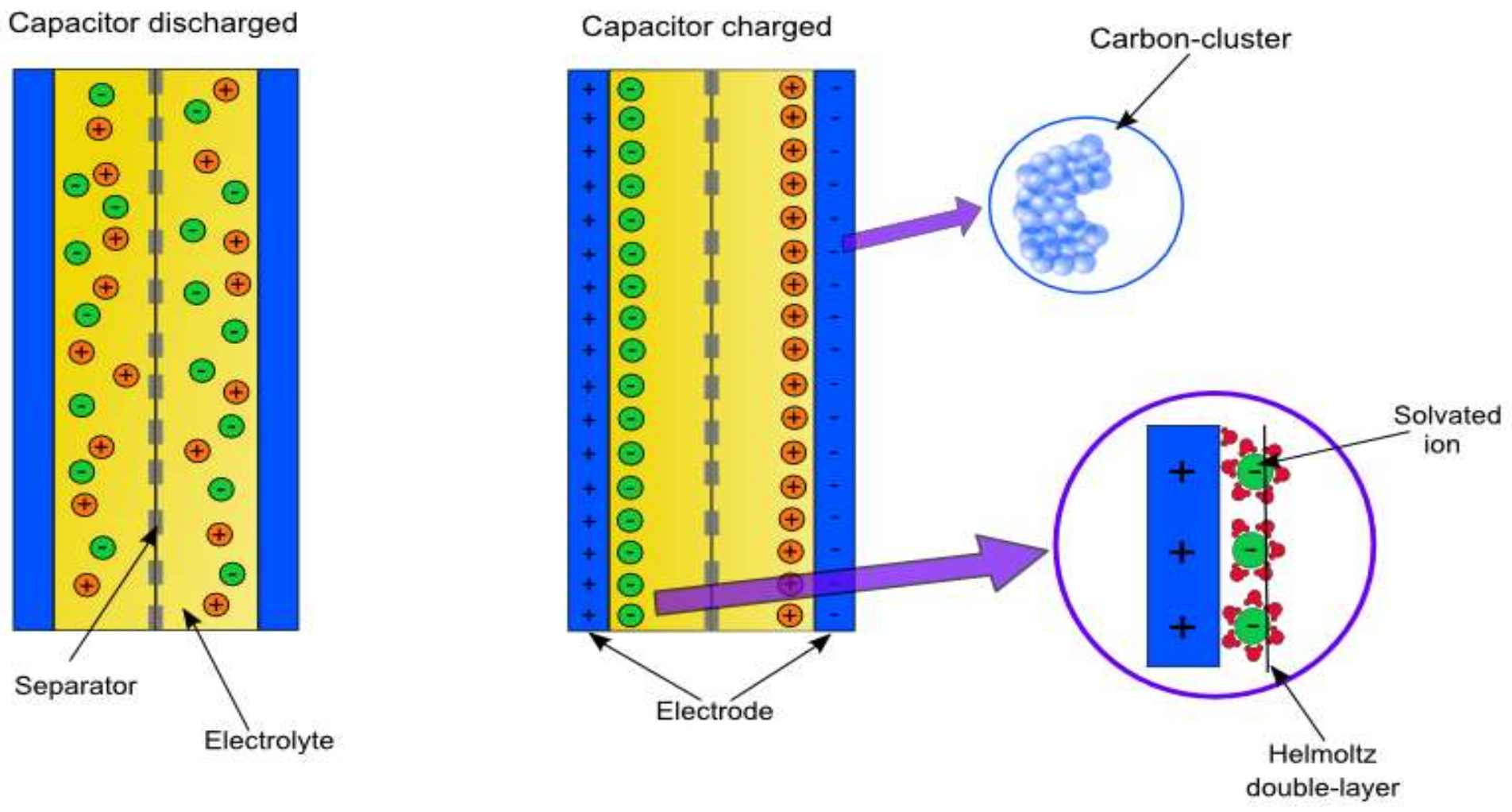
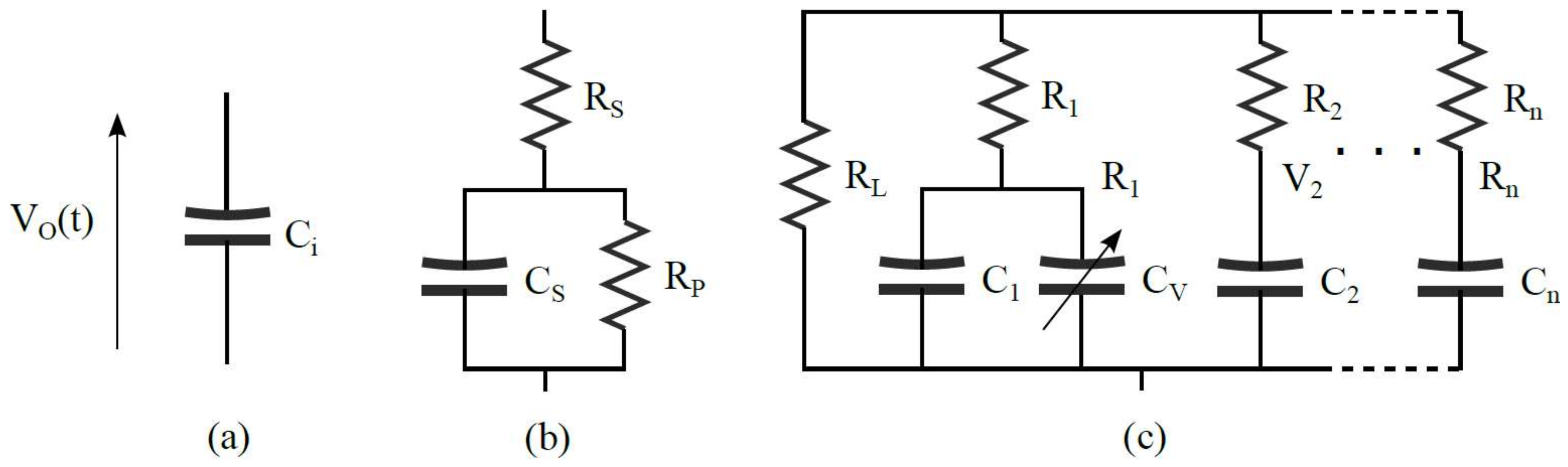
2.1. Equivalent Electrical Model
2.2. Mathematical Model
2.3. Machine Learning Algorithms
3. Experimental Tests
- Define the number of tests and their conditions and the measurement procedure.
- Design and build an evaluation fixture for testing different supercapacitors simultaneously.
- Implement the tests and obtain results.
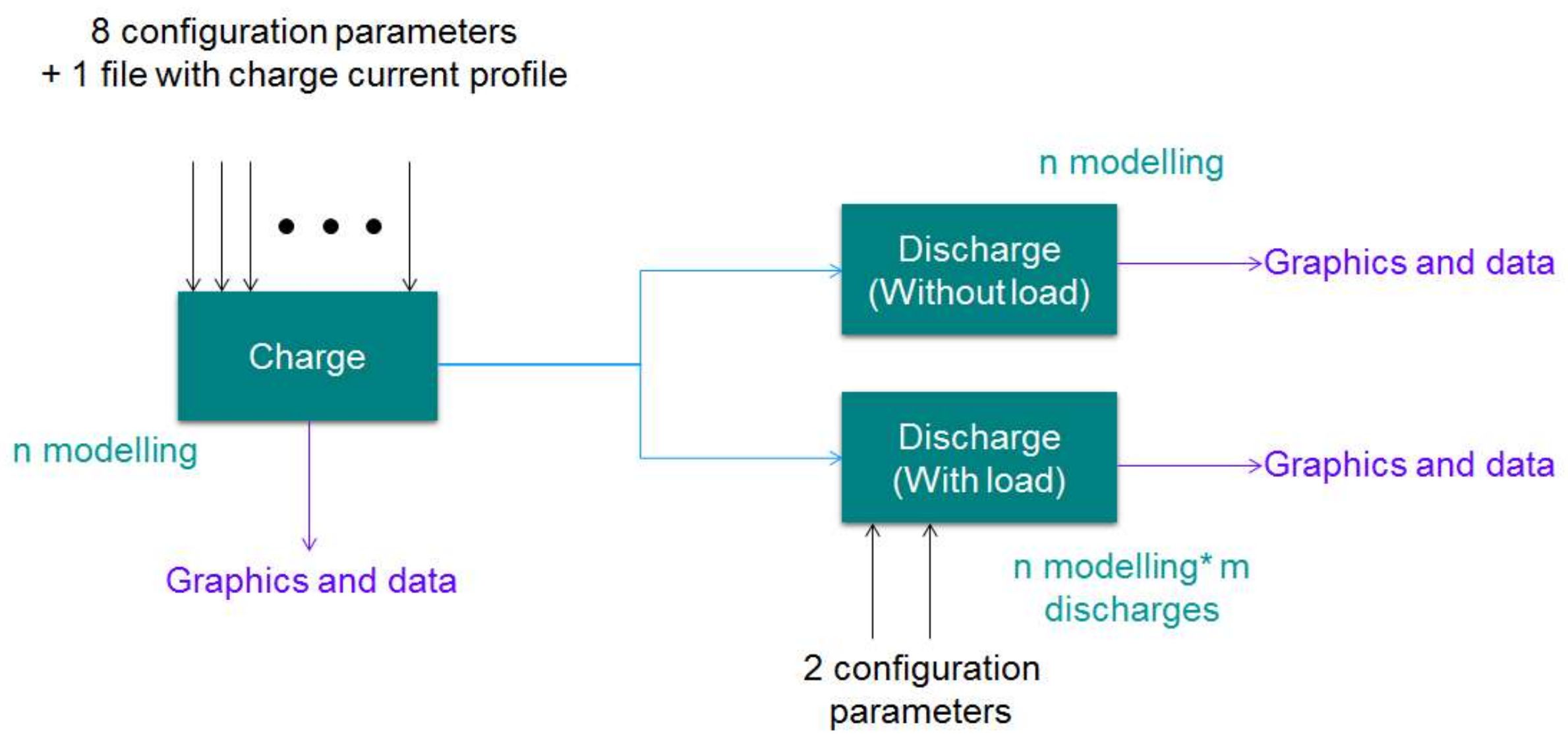
3.1. Test Definition
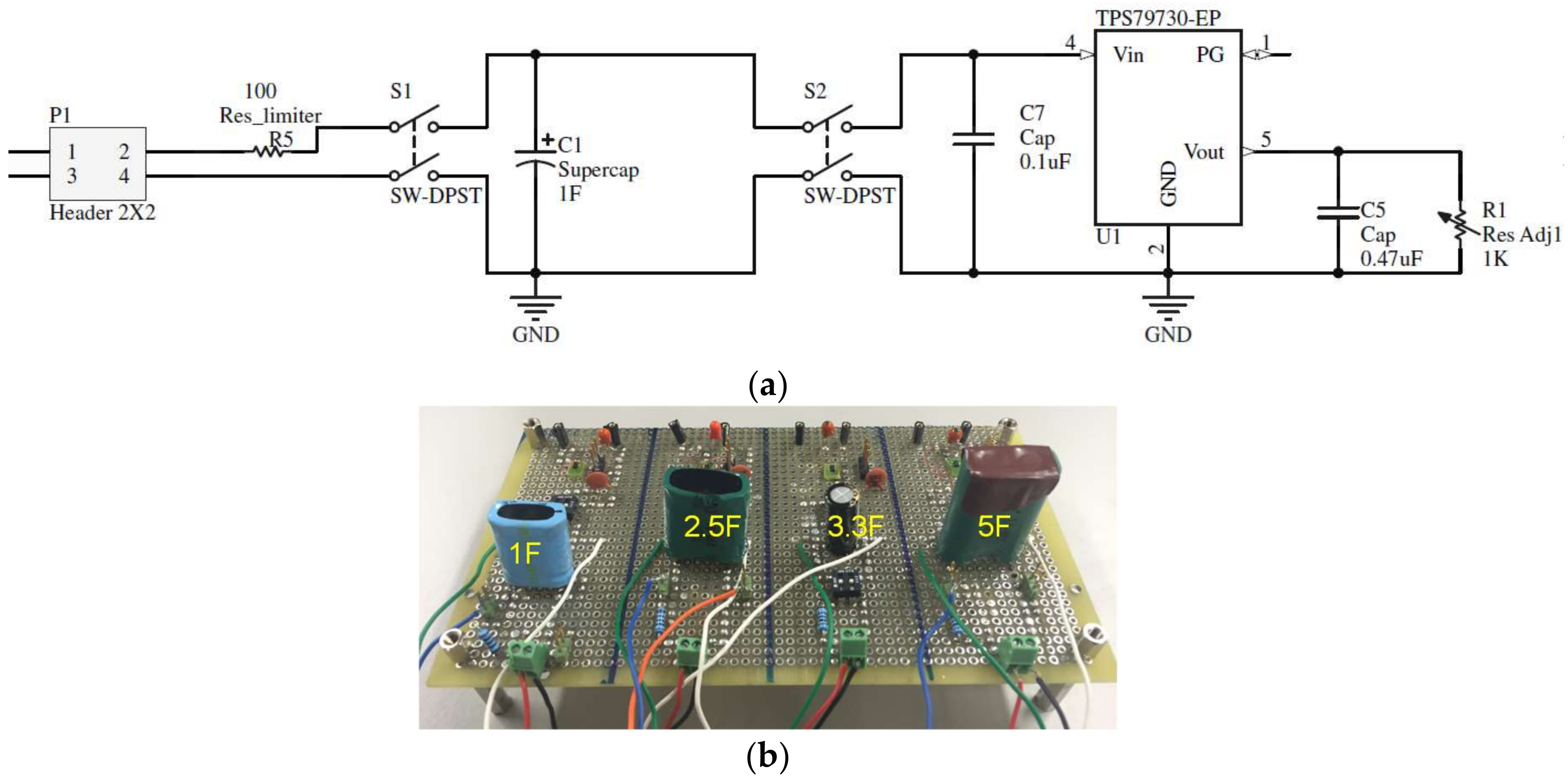
3.2. Evaluation-Board
- Charging: first switch on and second off.
- Self-discharge process: with the capacitor in charge state, the first switch is turned off.
- Load dependent discharge process: with the capacitor in charge state, the first switch is turned off and the second on.
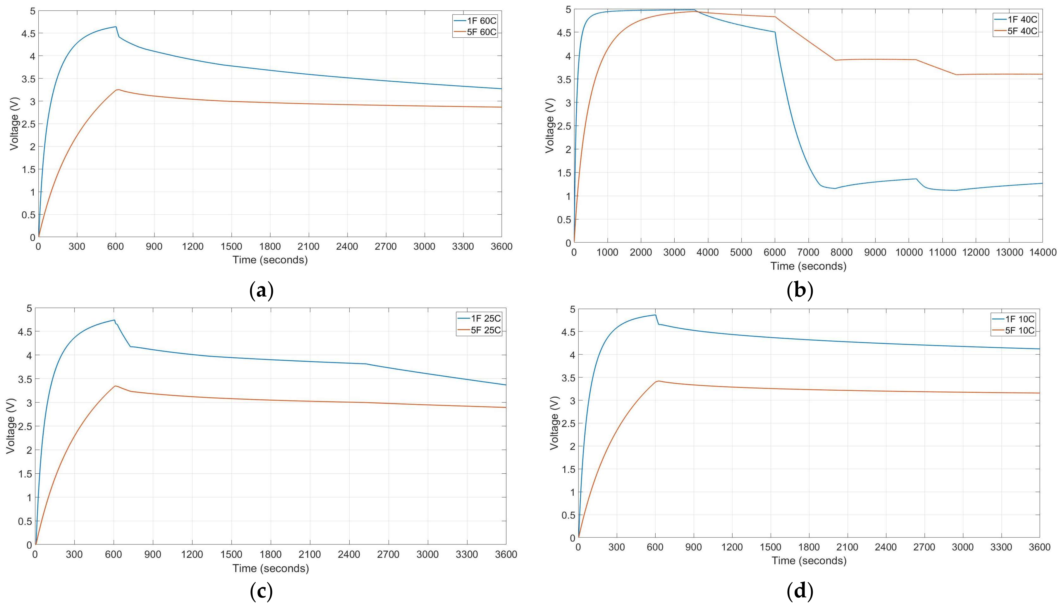
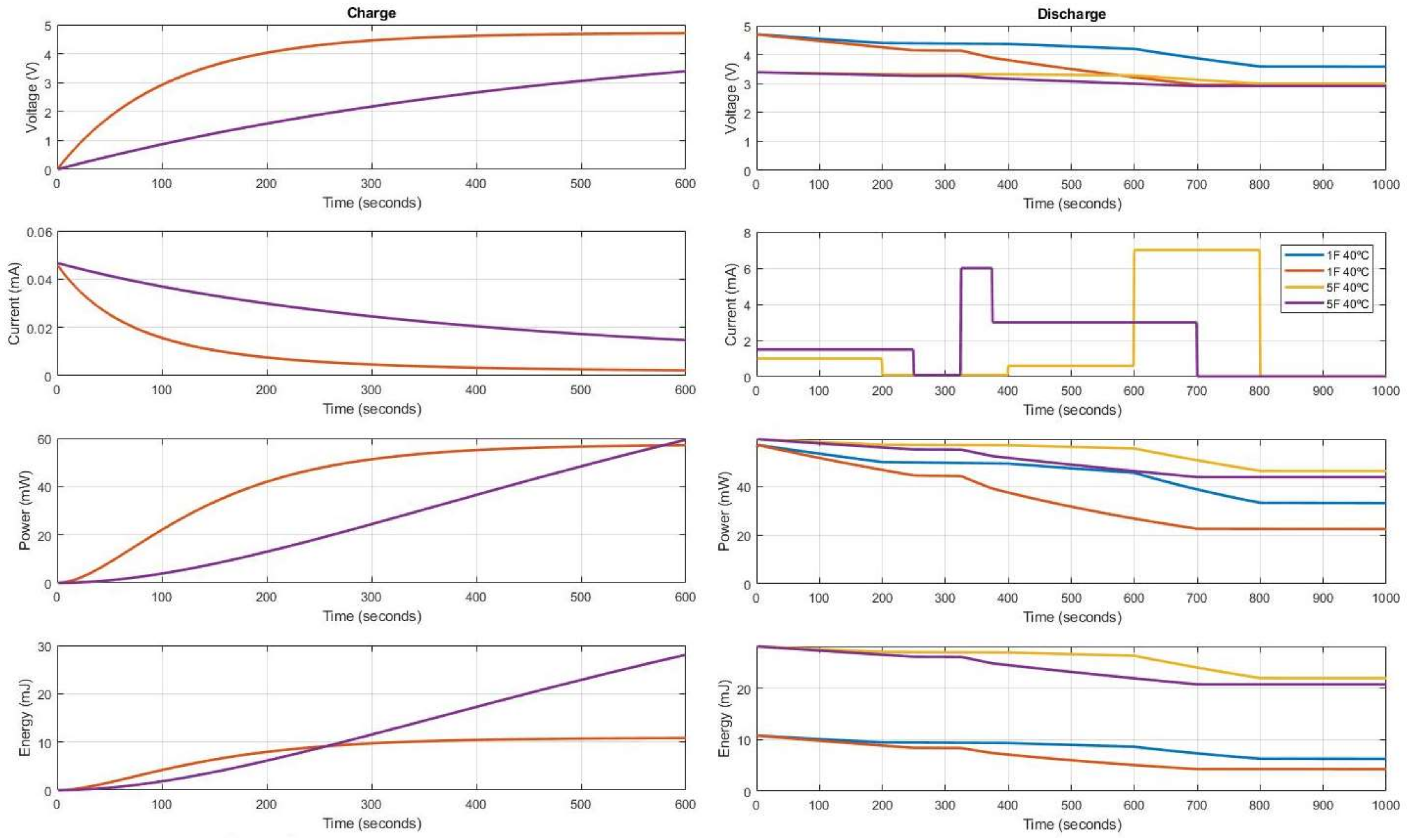
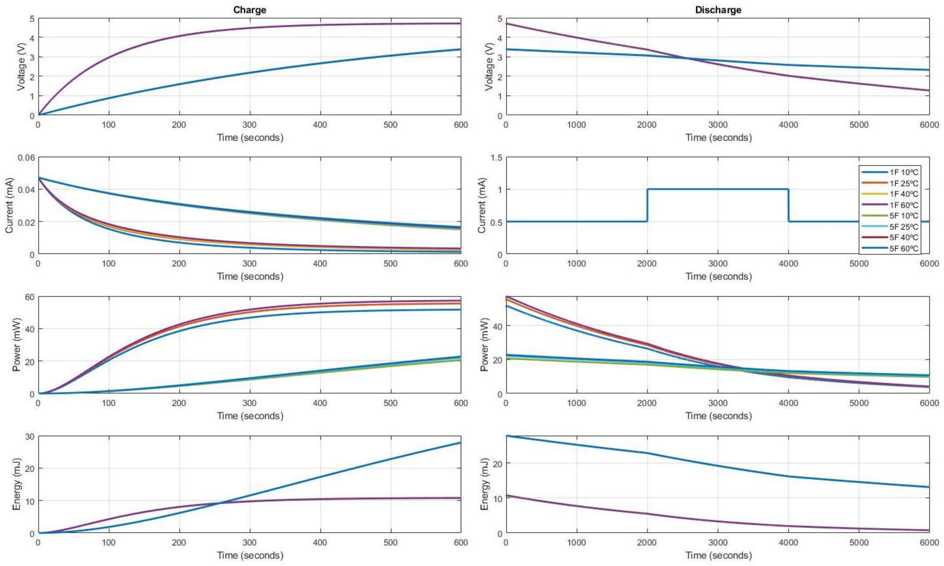
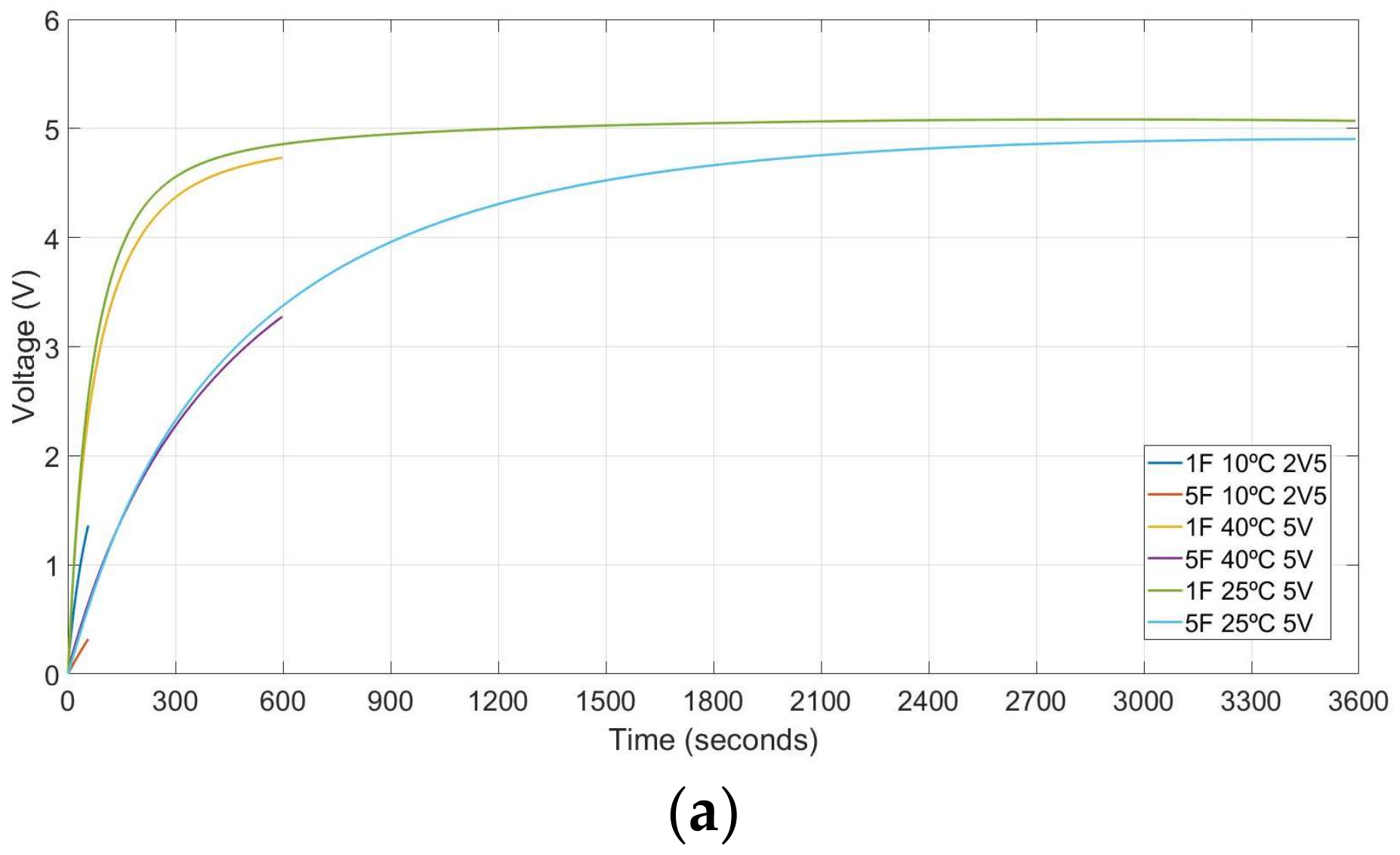
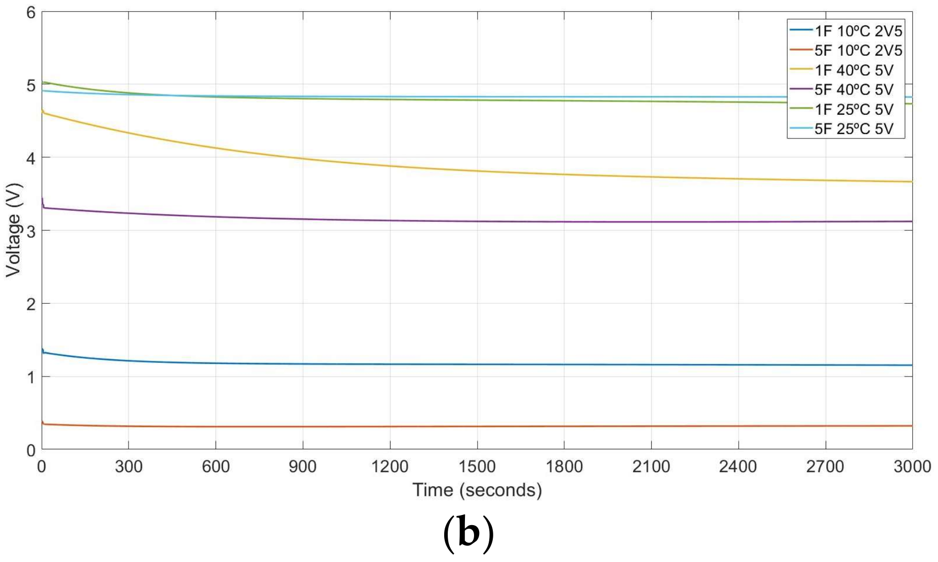
3.3. Test Results
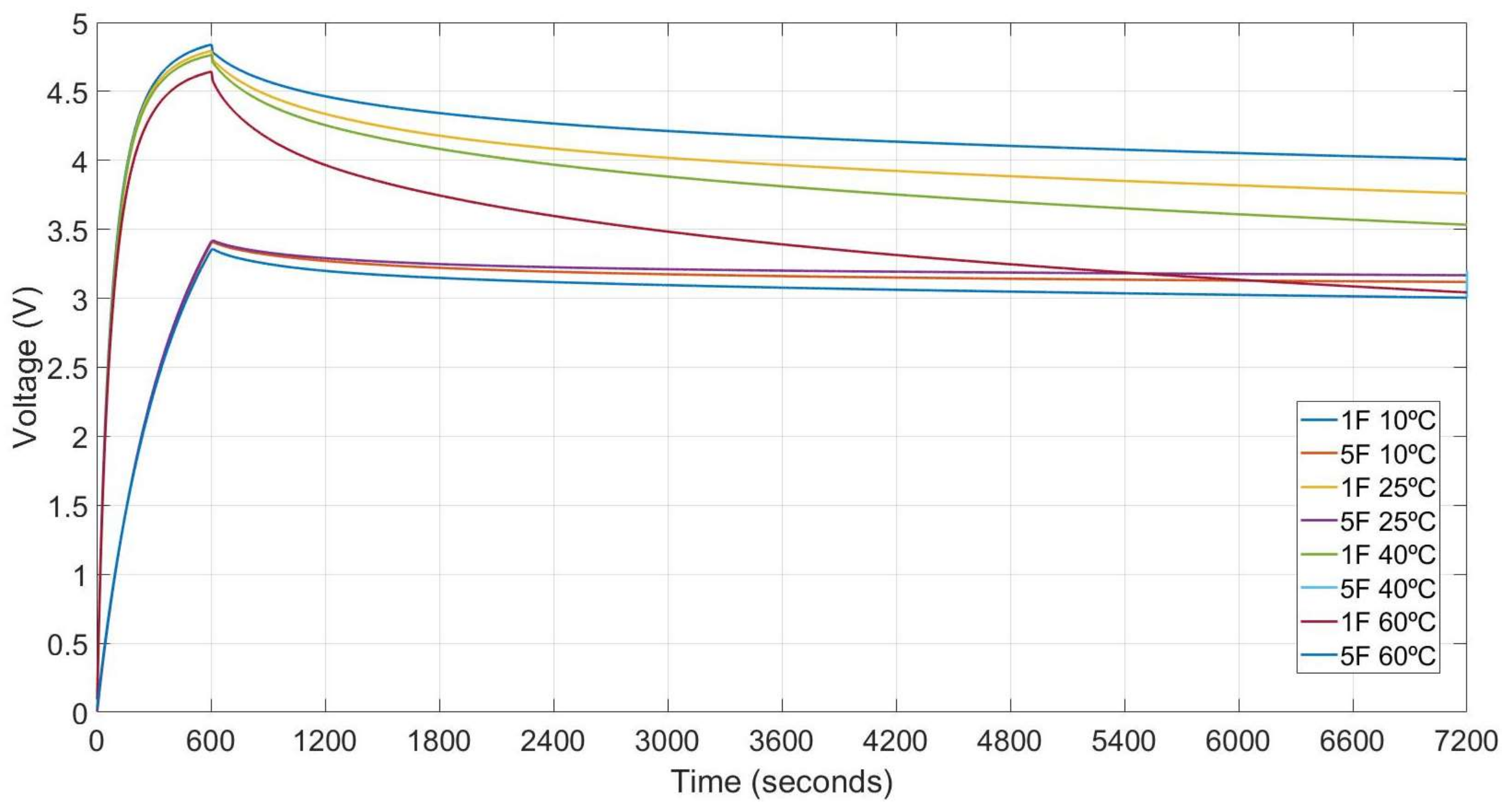
- The supercapacitor discharge curves are a function of the load and the discharge time.
- Changes of the ambient conditions and load produce significant deviation of the discharge characteristic.
- The accuracy of the machine learning model is a direct function of the amount data.
4. Electro-Mathematical Model
4.1. Equations
4.1.1. Capacity Ccomplet
4.1.2. Equivalent Series Resistance
4.1.3. Leakage Resistance
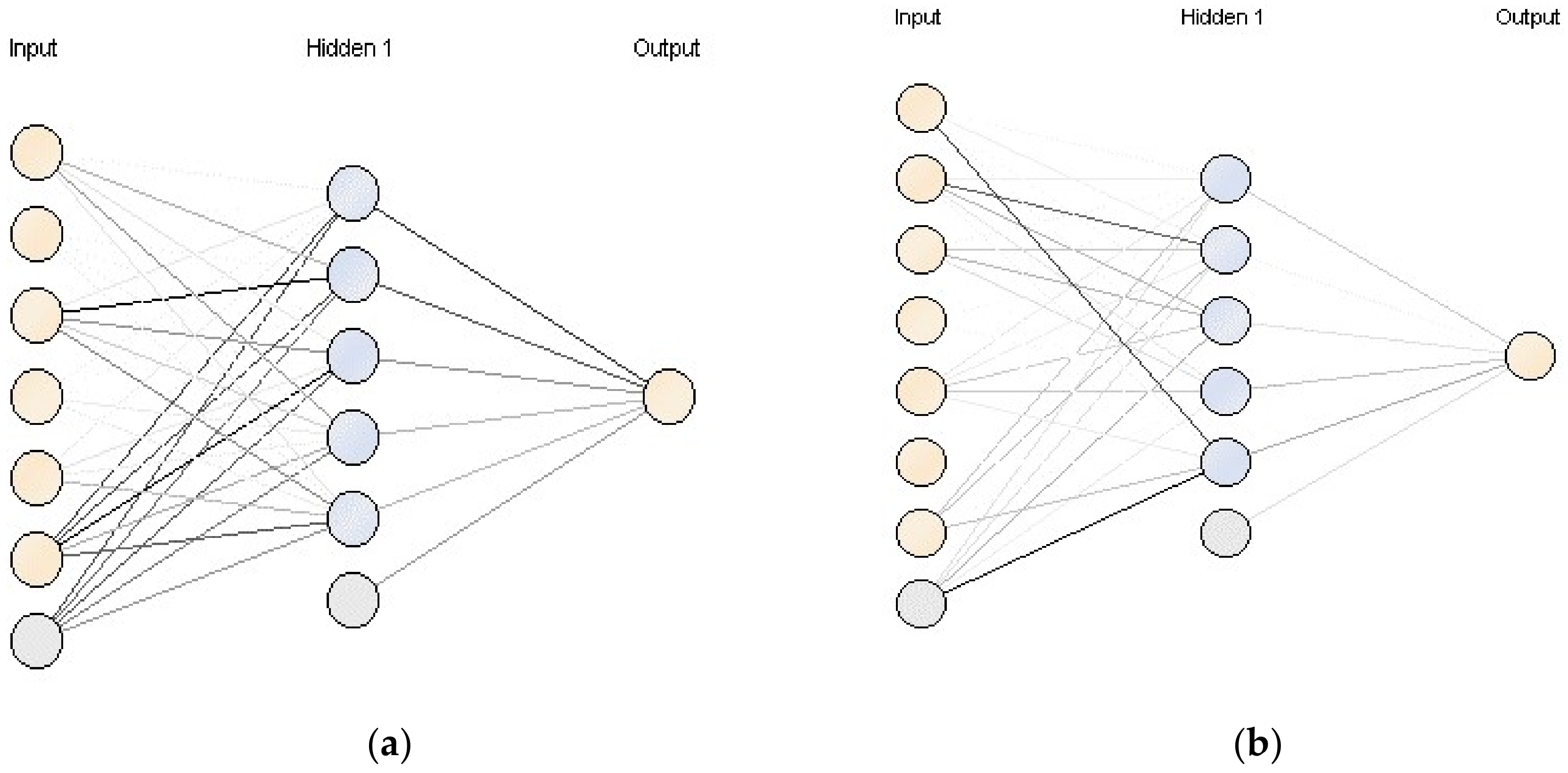
4.2. Model Architecture
4.3. Results
5. Machine Learning Model
5.1. Artificial Neural Network Setup
5.2. Objectives and Experimental Setup
5.3. Evaluation Method
- Estimate and compare the goodness of the model regarding future outcomes predictions.
- Select the model amongst two or more models.
5.4. Experimental Results
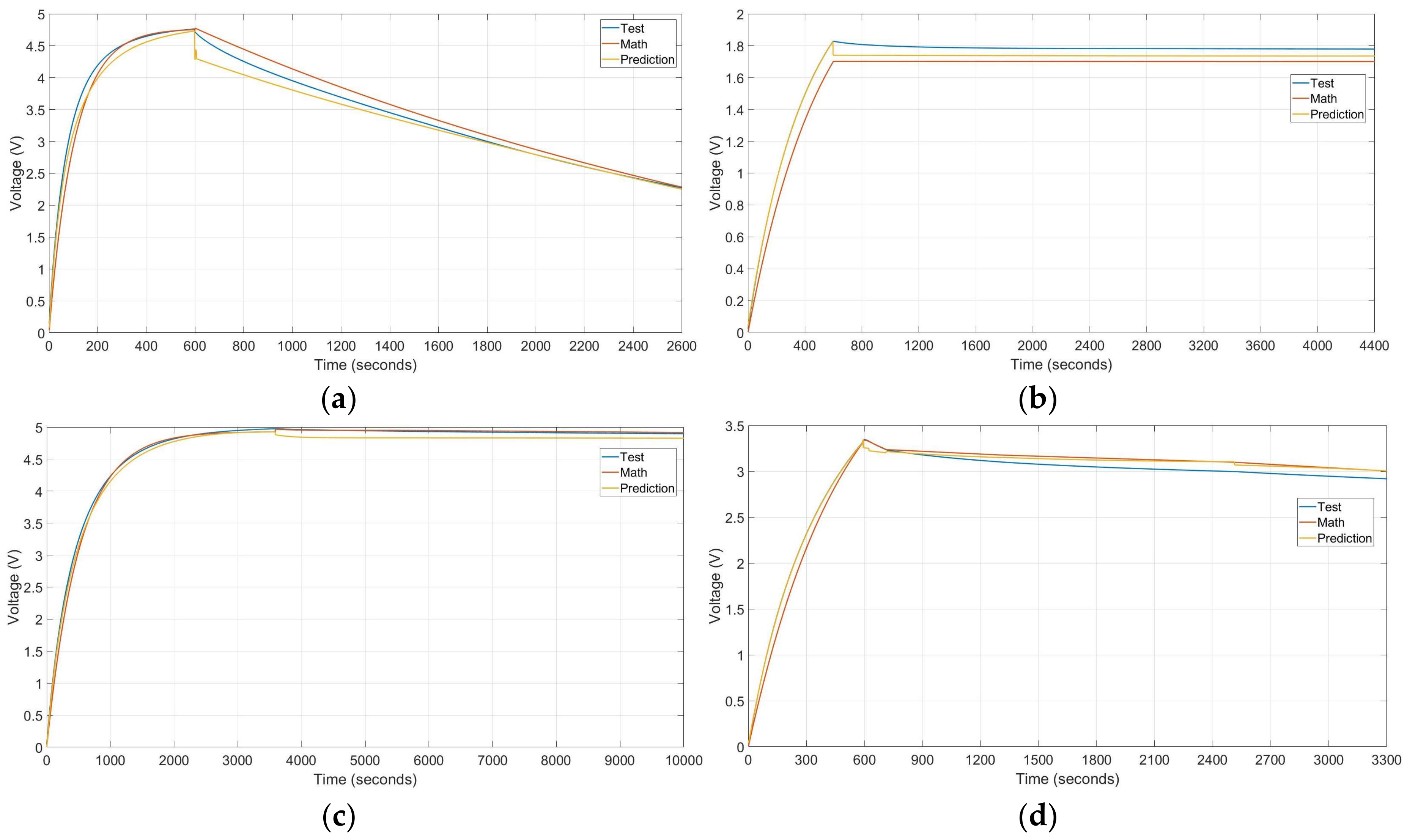
6. Validation of Models with Experimental Data
7. Conclusions
Author Contributions
Conflicts of Interest
References
- Rodrigues, L.M.; Montez, C.; Vasques, F.; Portugal, P. Experimental validation of a battery model for low-power nodes in Wireless Sensor Networks. In Proceedings of the 2016 IEEE World Conference on Factory Communication Systems (WFCS), Aveiro, Portugal, 3–6 May 2016; pp. 1–4. [Google Scholar]
- Zorbas, D.; Raveneau, P.; Ghamri-doudane, Y.; Douligeris, C. On the Optimal Number of Chargers in Battery-Less Wirelessly Powered Sensor Networks. In Proceedings of the 2017 IEEE Symposium on Computers and Communications (ISCC), Heraklion, Greece, 3–6 July 2017; pp. 1–6. [Google Scholar]
- Shnayder, V.; Hempstead, M.; Chen, B.; Allen, G.W.; Welsh, M. Simulating the power consumption of large-scale sensor network applications. In Proceedings of the SenSys '04 Proceedings of the 2nd International Conference on Embedded Networked Sensor Systems, Baltimore, MD, USA, 3–5 November 2004. [Google Scholar]
- Pourazarm, S.; Cassandras, C.G. Energy-based lifetime maximization and security of wireless-sensor networks with general nonideal battery models. IEEE Trans. Control Netw. Syst. 2017, 4, 323–335. [Google Scholar] [CrossRef]
- Wang, W.; Wang, N.; Vinco, A.; Siddique, R.; Hayes, M.; O’Flynn, B.; O’Mathuna, C. Super-capacitor and Thin Film Battery Hybrid Energy Storage for Energy Harvesting Applications. J. Phys. Conf. Ser. 2013, 476, 12105. [Google Scholar] [CrossRef]
- Sudevalayam, S.; Kulkarni, P. Energy harvesting sensor nodes: Survey and implications. IEEE Commun. Surv. Tutor. 2011, 13, 443–461. [Google Scholar] [CrossRef]
- Kumar, K.; Pahariya, Y. Analysis of Battery Lifetime Extension in a Small-Scale Wind-Energy System Using Supercapacitors. IEEE Trans. Energy Convers. 2012, 28, 24–33. [Google Scholar]
- El Mejdoubi, A.; Chaoui, H.; Sabor, J.; Gualous, H. Remaining Useful Life Prognosis of Supercapacitors Under Temperature and Voltage Aging Conditions. IEEE Trans. Ind. Electron. 2018, 65, 4357–4367. [Google Scholar] [CrossRef]
- Cammarano, A.; Petrioli, C.; Spenza, D. Pro-Energy: A novel energy prediction model for solar and wind energy-harvesting wireless sensor networks. In Proceedings of the 2012 IEEE 9th International Conference on Mobile Adhoc and Sensor Systems (MASS), Las Vegas, NV, USA, 8–11 October 2012; pp. 75–83. [Google Scholar]
- Park, S.W.; DeYoung, A.D.; Dhumal, N.R.; Shim, Y.; Kim, H.J.; Jung, Y.J. Computer Simulation Study of Graphene Oxide Supercapacitors: Charge Screening Mechanism. J. Phys. Chem. Lett. 2016, 7, 1180–1186. [Google Scholar] [CrossRef] [PubMed]
- Merlet, C.; Péan, C.; Rotenberg, B.; Madden, P.A.; Simon, P.; Salanne, M. Simulating supercapacitors: Can we model electrodes as constant charge surfaces? J. Phys. Chem. Lett. 2013, 4, 264–268. [Google Scholar] [CrossRef] [PubMed]
- Bertrand, N.; Sabatier, J.; Briat, O.; Vinassa, J.M. Fractional non-linear modelling of ultracapacitors. Commun. Nonlinear Sci. Numer. Simul. 2010, 15, 1327–1337. [Google Scholar] [CrossRef]
- Yang, H.; Zhang, Y. Analysis of Supercapacitor Energy Loss for Power Management in Environmentally Powered. IEEE Trans. Power Electron. 2013, 28, 5391–5403. [Google Scholar] [CrossRef]
- Cahela, D.; Tatarchuk, B. Overview of electrochemical double layer capacitors. In Proceedings of the IECON 97 23rd International Conference on Industrial Electronics, Control and Instrumentation, New Orleans, LA, USA, 14 November 1997; Volume 3, pp. 1068–1073. [Google Scholar]
- Saha, P. Equivalent Circuit Model of Supercapacitor for Self- Discharge Analysis—A Comparative Study. In Proceedings of the 2016 International Conference on Signal Processing, Communication, Power and Embedded System (SCOPES), Paralakhemundi, India, 3–5 October 2016; pp. 5–10. [Google Scholar]
- Amaral, A.M.R.; Cardoso, A.J.M. Simple experimental techniques to characterize capacitors in a wide range of frequencies and temperatures. IEEE Trans. Instrum. Meas. 2010, 59, 1258–1267. [Google Scholar] [CrossRef]
- Zubieta, L.; Bonert, R. Characterization of double-layer capacitors for power electronics applications. IEEE Trans. Ind. Appl. 2000, 36, 199–205. [Google Scholar] [CrossRef]
- Torregrossa, D. Improvement of Dynamic Modeling of Supercapacitor by Residual Charge Effect Estimation. Ind. Electron. 2014, 61, 1345–1354. [Google Scholar] [CrossRef]
- Kaus, M.; Kowal, J.; Sauer, D.U. Modelling the effects of charge redistribution during self-discharge of supercapacitors. Electrochim. Acta 2010, 55, 7516–7523. [Google Scholar] [CrossRef]
- Drummond, R.; Duncan, S.R. On Observer Performance for an Electrochemical Supercapacitor Model for Applications such as Fault Ride Through. In Proceedings of the 2015 IEEE Conference on Control Applications (CCA), Sydney, Australia, 21–23 September 2015; pp. 1260–1265. [Google Scholar]
- Chai, R.Z.; Zhang, Y. A Practical Supercapacitor Model for Power Management in Wireless Sensor Nodes. IEEE Trans. Power Electron. 2015, 30, 6720–6730. [Google Scholar] [CrossRef]
- Mitchell, T.M. Machine Learning in Ecosystem Informatics and Sustainability; McGraw-Hill Science/Engineering/Math: New York, NY, USA, 1997. [Google Scholar]
- Eddahech, A.; Briat, O.; Ayadi, M.; Vinassa, J.-M. Modeling and adaptive control for supercapacitor in automotive applications based on artificial neural networks. Electr. Power Syst. Res. 2014, 106, 134–141. [Google Scholar] [CrossRef]
- Wu, C.H.; Hung, Y.H.; Hong, C.W. On-line supercapacitor dynamic models for energy conversion and management. Energy Convers. Manag. 2012, 53, 337–345. [Google Scholar] [CrossRef]
- Golchoubian, P.; Azad, N.L.; Ponnambalam, K. Stochastic Nonlinear Model Predictive Control of Battery-Supercapacitor Hybrid Energy Storage Systems in Electric Vehicles. In Proceedings of the American Control Conference (ACC), Seattle, WA, USA, 24–26 May 2017. [Google Scholar]
- Ban, S.; Zhang, J.; Zhang, L.; Tsay, K.; Song, D.; Zou, X. Charging and discharging electrochemical supercapacitors in the presence of both parallel leakage process and electrochemical decomposition of solvent. Electrochim. Acta 2013, 90, 542–549. [Google Scholar] [CrossRef]
- Rajan, R.S.; Rahman, M.M. Lifetime Analysis of Super Capacitor for Many Power Electronics Applications. IOSR J. Electr. Electron. Eng. 2014, 9, 55–58. [Google Scholar] [CrossRef]
- Kötz, R.; Hahn, M.; Gallay, R. Temperature behavior and impedance fundamentals of supercapacitors. J. Power Sources 2006, 154, 550–555. [Google Scholar] [CrossRef]
- Murray, D.B.; Hayes, J.G. Cycle testing of supercapacitors for long-life robust applications. IEEE Trans. Power Electron. 2015, 30, 2505–2516. [Google Scholar] [CrossRef]
- Liu, K.; Zhu, C.; Lu, R.; Chan, C.C. Improved study of temperature dependence equivalent circuit model for supercapacitors. IEEE Trans. Plasma Sci. 2013, 41, 1267–1271. [Google Scholar]
- Miller, J.M. Ultracapacitor Applications Ultracapacitor Applications; The Institution of Engineering and Technology: London, UK, 2011; pp. 37–91. [Google Scholar]
- Diab, Y.; Venet, P.; Gualous, H.; Rojat, G. Self-discharge characterization and modeling of electrochemical capacitor used for power electronics applications. IEEE Trans. Power Electron. 2009, 24, 510–517. [Google Scholar] [CrossRef]
- Hofmann, M.; Klinkenberg, R. RapidMiner: Data Mining Use Cases and Business Analytics Applications; CRC Press: Boca Raton, FL, USA, 2013. [Google Scholar]
- Eddahech, A.; Ayadi, M.; Briat, O.; Vinassa, J.M. Online parameter identification for real-time supercapacitor performance estimation in automotive applications. Int. J. Electr. Power Energy Syst. 2013, 51, 162–167. [Google Scholar] [CrossRef]
- Berrueta, A.; Martín, I.S.; Hernández, A.; Ursúa, A.; Sanchis, P. Electro-thermal modelling of a supercapacitor and experimental validation. J. Power Sources 2014, 259, 154–165. [Google Scholar] [CrossRef]
- Zhang, L.; Hu, X.; Wang, Z.; Sun, F.; Dorrell, D.G. Fractional-order modeling and State-of-Charge estimation for ultracapacitors. J. Power Sources 2016, 314, 28–34. [Google Scholar] [CrossRef]


| Variable | Temperature (°C) | Charge Voltage (V) | Charge Time (s) | Supercapacitor Values (F) | Discharge Time (s) |
|---|---|---|---|---|---|
| Test conditions | 10, 25, 40, 60 | 2.5, 5 | 60, 600, 3600 | 1 F, 5 F | Infinity load, fixed value load, variable load steps |
| Parameter | Description | Value |
|---|---|---|
| hidden_layers | Name and size of the hidden layers. | (number of attributes + number of classes)/2 + 1 |
| training_cylces | Number of training cycles used for the training phase. | 500 |
| learning_rate | Weight rate change of each step | 0.3 |
| momentum | It adds a fraction of the previous weight update to the current one. | 0.2 |
| decay | Flag to decrease or not the learning rate | False |
| shuffle | Flag to shuffle or not the data before learning | Yes |
| normalize | The Neural Net operator uses a usual sigmoid function as the activation function. Therefore, the value range of the attributes should be scaled to −1 and +1. This can be done through the normalize parameter. Normalization is performed before learning. Although it increases runtime, but it is necessary in most cases | Yes |
| error_epsilon | optimization training error target value. | 1 × 10⁻⁵ |
| use_local_random_seed | Flag to use a random seed for randomization | No |
| local_random_seed | Local random seed. It is only used if use_local_random_seed is set to TRUE | - |
| Variable | Data Type | Values |
|---|---|---|
| Time | Integer | |
| Temperature (°C) | Integer | 10, 25, 40, 60 |
| Voltage (V) | Integer | 2.5, 5 |
| Charge Time (s) | Integer | 60, 600, 3600 |
| Capacitance | Integer | 1 F, 5 F |
| Charge current | Real | [0–45] mA |
| Variable | Data Type | Values | RMSE | Sd |
|---|---|---|---|---|
| 1st | Charge | For all conditions of the test | 0.007 | 0.005 |
| Discharge | For all conditions of the test | 0.222 | 0.035 | |
| 2nd | Discharge | Charge-Time (60) | 0.007 | 0.002 |
| Charge-Time (600) | 0.232 | 0.091 | ||
| Charge-Time (3600) | 0.111 | 0.024 | ||
| 3rd | Discharge and charge curve at the same model | Charge-Time (60) | 0.021 | 0.002 |
| Charge-Time (600) | 0.213 | 0.071 | ||
| Charge-Time (3600) | 0.244 | 0.098 |
| Statistical Technique | (a) Example | (b) Example | (c) Example | (d) Example | Average All | ||||||
|---|---|---|---|---|---|---|---|---|---|---|---|
| Pred. | Math | Pred. | Math | Pred. | Math | Pred. | Math | Pred. | Math. | ||
| Charge | RMSE | 0.137 | 0.204 | 0.113 | 0.178 | 0.007 | 0.145 | 0.005 | 0.134 | 0.052 | 0.146 |
| MSE | 0.019 | 0.042 | 0.013 | 0.032 | 0.0001 | 0.021 | 0.00002 | 0.018 | 0.005 | 0.023 | |
| MAE | 0.123 | 0.125 | 0.103 | 0.167 | 0.006 | 0.114 | 0.004 | 0.118 | 0.047 | 0.101 | |
| MAPE | 3.606 | 5.354 | 4.689 | 11.642 | 0.655 | 4.387 | 1.514 | 8.607 | 3.549 | 5.712 | |
| Discharge | RMSE | 0.119 | 0.123 | 0.071 | 0.083 | 0.157 | 0.048 | 0.074 | 0.086 | 0.099 | 0.134 |
| MSE | 0.014 | 0.015 | 0.005 | 0.007 | 0.025 | 0.002 | 0.005 | 0.007 | 0.017 | 0.031 | |
| MAE | 0.079 | 0.111 | 0.064 | 0.078 | 0.143 | 0.047 | 0.069 | 0.081 | 0.090 | 0.128 | |
| MAPE | 2.013 | 3.210 | 2.211 | 2.653 | 3.659 | 1.230 | 2.272 | 2.685 | 2.819 | 3.792 | |
| Model Type | Ref. Numb. | Statistical Error | Ref. Result | This Work Result |
|---|---|---|---|---|
| Electro-mathematical | [12] | Deviation | 3–7% | 2.35% |
| Electro-mathematical | [34] | Deviation | 2.56% | 2.35% |
| Electro-mathematical | [35] | RMSE | 0.65 | 0.071–0.204 |
| M.L. → ANN | [23] | MSE | 0.089 | 0.005–0.017 |
| M.L. → Kalman Filtering | [36] | MAE | 0.50 | 0.047–0.090 |
| RMSE | 0.63 | 0.052–0.099 |
© 2018 by the authors. Licensee MDPI, Basel, Switzerland. This article is an open access article distributed under the terms and conditions of the Creative Commons Attribution (CC BY) license (http://creativecommons.org/licenses/by/4.0/).
Share and Cite
Pozo, B.; Garate, J.I.; Ferreiro, S.; Fernandez, I.; Fernandez de Gorostiza, E. Supercapacitor Electro-Mathematical and Machine Learning Modelling for Low Power Applications. Electronics 2018, 7, 44. https://doi.org/10.3390/electronics7040044
Pozo B, Garate JI, Ferreiro S, Fernandez I, Fernandez de Gorostiza E. Supercapacitor Electro-Mathematical and Machine Learning Modelling for Low Power Applications. Electronics. 2018; 7(4):44. https://doi.org/10.3390/electronics7040044
Chicago/Turabian StylePozo, Borja, Jose Ignacio Garate, Susana Ferreiro, Izaskun Fernandez, and Erlantz Fernandez de Gorostiza. 2018. "Supercapacitor Electro-Mathematical and Machine Learning Modelling for Low Power Applications" Electronics 7, no. 4: 44. https://doi.org/10.3390/electronics7040044
APA StylePozo, B., Garate, J. I., Ferreiro, S., Fernandez, I., & Fernandez de Gorostiza, E. (2018). Supercapacitor Electro-Mathematical and Machine Learning Modelling for Low Power Applications. Electronics, 7(4), 44. https://doi.org/10.3390/electronics7040044